Comparison of Naive Bayes and SVM Classifiers in ...

See discussions, stats, and author profiles for this publication at: https://www.researchgate.net/publication/258885305

Comparison of Naive Bayes and SVM Classifiers in Categorization of Concept Maps Article · January 2013

CITATIONS

READS

0

2,307

3 authors: Krunoslav Zubrinic

Mario Milicevic

University of Dubrovnik

University of Dubrovnik

16 PUBLICATIONS 32 CITATIONS

18 PUBLICATIONS 28 CITATIONS

SEE PROFILE

SEE PROFILE

Ivona Zakarija University of Dubrovnik 11 PUBLICATIONS 4 CITATIONS SEE PROFILE

All content following this page was uploaded by Krunoslav Zubrinic on 29 March 2017. The user has requested enhancement of the downloaded file. All in-text references underlined in blue are added to the original document and are linked to publications on ResearchGate, letting you access and read them immediately.

INTERNATIONAL JOURNAL OF COMPUTERS Issue 3, Volume 7, 2013

Comparison of Na¨ıve Bayes and SVM Classifiers in Categorization of Concept Maps Krunoslav Zubrinic, Mario Milicevic and Ivona Zakarija

Abstract— Concept map is a graphic tool which describes a logical structure of knowledge in the form of connected concepts. Many persons create and use concept maps as planning, knowledge representation or evaluation tool, and store them in a public repository. In such environment contents and quality of these maps vary. When user wants to use specific map, they have to know to which domain that map belongs. Many creators do not pay enough attention to complete and accurate labeling of their documents. Manually categorization of maps in large repository is almost impossible as it is a very long and demanding procedure. In such environment automatic classification of concept maps according to their content can help users to identify the relevant map. There are very few researches on automatic classification of concept maps. In this paper we propose method for automatic categorization of concept maps using simple bag of words. In our experiment, data for classification are taken from a set of public available CMs Fetched maps are filtered by language and parsed. Concepts’ labels are extracted from filtered set of CMs, preprocessed and prepared for classification. The most important features are selected and data are prepared for learning and classification. Training and classification are performed using na¨ıve Bayes and SVM classifiers. Achieved results are promising, and with further data preprocessing and adjustment of the classifiers we consider that they can be improved. Keywords—Classification, concept map, data mining, na¨ıve Bayes, SVM, text mining.

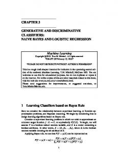
I. I NTRODUCTION ONCEPT map (CM) is a form of graphical representation of relationships among concepts. It is used as a tool to describe a logical structure of knowledge. As a knowledge representation tool they have been successfully used for organizing and representing information in different areas, including education, knowledge management, data modeling, business and intelligence. Concept typically represents ideas and information in the form of boxes or circles that are connected with labeled arrows. The relationships between concept pairs can be labeled with linking phrases, while a CM can be hierarchically organized. Concepts are usually labeled by nouns or noun phrases [1], [2].

C

Manuscript received June 26, 2013. K. Zubrinic is with the Department of Electrical Engineering and Computing, University of Dubrovnik, Cira Carica 4, Dubrovnik, Croatia (e-mail: [email protected]). M. Milicevic is with the Department of Electrical Engineering and Computing, University of Dubrovnik, Cira Carica 4, Dubrovnik, Croatia (e-mail: [email protected]). I. Zakarija is with the Department of Electrical Engineering and Computing, University of Dubrovnik, Cira Carica 4, Dubrovnik, Croatia (e-mail: [email protected]).

Fig. 1 shows an example of CM that explains a way of reproduction in flowering plants [3].

Fig. 1.

Example of CM

There has been a remarkable growth in the use of CMs across the world over the past decade. During concept mapping process, the creator constructs a two dimensional representation of concepts and their relationships. That flexibility in constructing of CMs is commonly regarded as an advantage of concept mapping for use in many fields, as the created map reflects what the creator knows of the subject field. Given that each person’s understanding of a domain is different, even if people construct CMs on the same topic, the maps constructed by individuals are different [4]. In the environments where many persons or different software applications represent information in a form of a CM, contents and the quality of these maps may vary [2], [5] . Some authors do not care enough about correct and complete labeling of their documents using semantic meta-data [6]. When user wants to access elements of some map, they have to have some sense of the map’s content and scope. It is very difficult and time consuming for them to browse through details of every map in large repository. It would be very useful if the system could automatically give information on the content and scope of every CM. CM’s semantic tags such as title, subject or description can be used for scope identification. Multilingual environments where maps can be created using terms written in different languages increases that problem. As manual categorization of maps in large repository can be a very long and demanding procedure, automatic classification of CMs can help user to select and identify topically relevant CMs. Possible application of that procedure includes assessing CM similarity, structuring and facilitating access to CMs, or automatic proposing and finding additional materials that

109

INTERNATIONAL JOURNAL OF COMPUTERS Issue 3, Volume 7, 2013

could be included in existing CM. The automatic classification of CMs has been studied by several researchers who were focused on development and evaluation of a tool for automatic classification of CMs based on a topological taxonomy [4], [7], similarity of concepts [8] or determining differences between groups of maps based on connections among concepts [9]. In text categorization, several researches treat document as a collection of concepts, rather than independent words [10], [11]. In this research we argue that it is possible to classify CMs if we consider them as a flat, non-hierarchical map of concepts. We use simple bag of words model, which simplifies representation of a CM as an unordered collection of nouns or noun phrases that form concepts’ labels. II. P ROBLEM FORMULATION Creator of CM who create map using concept mappings application can enrich content of created map with semantic meta tags, such as title, subject or description. These elements can help a user to understand the scope and structure of created CM. At the beginning of this research, we try to figure out how many of CM authors enter that data in their maps. We made a brief analysis of these elements in a set of 600 randomly selected CMs retrieved from public CMAP servers1 . We checked presence and correctness of four semantic tags: title, language, keywords and descriptions. As correct title we count one that is entered in a CM, and the meaning of which is connected with content of a CM. Titles filled with author’s name or text such as ”Untitled“ or ”0“ are counted as incorrect. We considered that language is correct if majority of concepts and relationship are labeled using the labeled language. For other elements we check only their presence. As shown in Fig. 2., creators of a CM frequently fill only title tag, in 92% of observed CMs. We checked whether the CM is labeled with the correct language, and found rather bad correctness, as language is correct in 76% of the set. The reason for that is that some creators, when using concept mappings applications, leave English as default language, regardless of the language used. Other observed tags (description and keywords) are filled very rarely, in 15% and 9% of maps (respectively). One of the reasons why the title is entered in so many maps is that the title is required in all concept mappings application. Although that analysis is not very detailed, on the basis of it we have come to the conclusion that meta tags of CMs in many cases are not detailed enough to identify maps by content. Marking the map in some other way according to their content can help users to identify the relevant map. Automatic classification is a learning process during which a program recognizes the characteristics that distinguish each category from others and constructs a classifier when given a set of training examples with class labels. 1 Public

CMAP servers used at http://cmapspublic.ihmc.us/, http://cmapspublic3.ihmc.us/

in this study can be accessed http://cmapspublic2.ihmc.us/ and

Fig. 2.

Percentage of meta tag entry in a set of randomly selected CMs

Text classification is the task of classifying a document under a predefined category. If di is a document of the entire set of documents D = {d1 , d2 , ..., dn } and C = {c1 , c2 , ..., cm } is the set of all the categories, then text classification assigns one category cj to a document di [12]. The goal of classification is to find function γ : D → C that will correctly classify a document di from a set of documents for classification in the appropriate class cj . Application of this approach to the CMs can help in automatic categorizing of maps on the basis of similarity of their content. In that way it is possible to reduce the drawbacks of manual tagging. In this research we classify CMs using simple bag of words approach successfully used in classification of text documents. Using that approach we simplify representation of a CM as an unordered collection of concepts’ labels. Words used for classification are taken from concepts’ labels, while relationships labels are not used. There are two reasons why names of relationships are not used. The first reason is simplicity, as the most of information on CM can be drawn from concepts’ names (which are usually nouns and noun phrases). The second reason is fact that in many CM’s created in real world, relationships are not labeled. III. D ESCRIPTION OF USED CLASSIFIERS In our experiment we used two types of classifiers; na¨ıve Bayes (NB) [13] and Support Vector Machine (SVM) [14] that were successfully used in previous researches in text classification. A. Na¨ıve Bayes NB is simple Bayesian supervised classifier that assumes that all attributes are independent of each other, given the context of the class [13].

110

INTERNATIONAL JOURNAL OF COMPUTERS Issue 3, Volume 7, 2013

P (x|y = c) =

D Y

P (xi |y) = c

(1)

i=1

This is the so-called NB assumption which is rarely true in the most real-world situations. Despite this, NB often performs classification very well [15]. Because of that assumption, the parameters for each attribute can be learned separately, and this greatly simplifies learning, especially when the number of attributes is large. Based on NB assumption, probability of a document given its class can be calculated as product of the probability of the attribute values over all word attributes. Given estimates of parameters calculated from the training documents, classification can be performed on test documents by calculating the posterior probability of each class given the evidence of the test document, and selecting the class with the highest probability [13]. In this model a document is a sequence of words taken from the same vocabulary V and lengths of documents are independent of class. Assumption is that the probability of each word event in a document is independent of the word’s context and position in the document. Thus, each document di is drawn from a multinomial distribution of words and represented in the form of bag of words [13]. P (di |cj ; θ) = P (|di |)|di |!

|V | N Y P (di |cj ; θ) it i=1

Nit !

(2)

The probabilities of each word are parameters of the generative component for P each class θwt |cj = P (wt |cj ; θ) where 0 ≤ θwt |cj ≤ 1 and t θwt |cj = 1. Optimal estimates for these parameters a calculated from a set of labeled training data, and the estimate of the probability of word wt in class cj is: ˆ θˆwt |cj = P (wt |cj ; θ)

P|D| 1 + i=1 Nit P (cj |di ) P|V | P|D| |V | + s=1 i=1 Nis P (cj |di )

(3)

Given estimates of parameters calculated from the training documents, classification can be performed on test documents by calculating the posterior probability of each class given the evidence of the test document, and selecting the class with the highest probability using Bayes’ rule [13]. ˆ ˆ ˆ (cj |θ)P (di |cj ; θj ) P (cj |di ; θ) ˆ P (di |θ)

and this information on frequency of each word can help in classification. Documents classification is an example of a domain with a large number of attributes. Those attributes are words, and the number of different words in a document can be large. NB has been successfully applied to document classification in many researches [13], [15], [16], [17]. B. Support Vector Machine SVM [14] is a supervised learning algorithm for classification problems. It is based on the structural risk minimization principle from computational learning theory. The idea is to find a hypothesis for which we can guarantee the lowest true error. The true error of a hypothesis is the probability that this hypothesis will make an error on an unseen and randomly selected test example. One important property of SVMs is that their ability to learn can be independent of the dimensionality of the feature space. SVMs measure the complexity of hypotheses based on the margin with which they separate the data, and not the number of features [18]. In its simplest, linear form, an SVM is a hyperplane that separates a set of positive examples from a set of negative examples with maximum margin. The bounded region is called the margin, and samples on the margin are called the support vectors [19]. In the linear case, the margin is defined by the distance of the hyperplane to the nearest of the positive and negative examples. Given some training data D, a set of n points of the form n

D = {(xi , yi )|xi ∈ Rp , yi ∈ {−1, 1}}i=1

where the yi is either 1 or −1, indicating the correct output of SVM classification to which the training example xi belongs. The value yi is +1 for the positive examples in a class, and -1 for negative examples. Each xi is a p-dimensional real vector. The formula for the output of a linear SVM is u = w · x − b where · is a dot product, w is the normal vector to hyperplane, and x is the input vector. The separating hyperplane is the plane where u = 0, and nearest points lie on the planes where 1 u = ±1. The parameter m = kwk 2 determines the margin, and maximizing margin can be expressed solving following optimization problem [20]: 1 min kwk2 ; yi (w · xi − b) ≥ 1, ∀i w,b 2

(4)

In our research we use multivariate Bernoulli and multinomial model of NB. In the multivariate Bernoulli model, a document is represented with binary vector of words. Each dimension of the space corresponds to word vocabulary. Dimension of the vector for document is either 0 or 1, indicating whether the word occurs at least once in the document. Unlike that, multinomial model of NB uses representation of a document as a vector of word occurrences,

(5)

(6)

SVM is fundamentally a two-class classifier. In practice we often have problems involving classification to more than two classes. In order to build a multi-class classifier, there have been proposed different approaches. Common approach is to construct a multi-class classifier by combining several binary classifiers [21] . Topic identification with SVM implies a kind of semantic space in the sense that the learned hyper plane separates documents which belong to different topics in the input space.

111

INTERNATIONAL JOURNAL OF COMPUTERS Issue 3, Volume 7, 2013

When learning text classifiers, one has to deal with a great number of features [19]. One way to avoid high dimensional input spaces is to assume that most of the features are irrelevant. Unfortunately, in text categorization there are only few irrelevant features. Results of researches show that even features ranked lowest still contain considerable information and are somewhat relevant [18]. Since SVMs use over fitting protection, which does not necessarily depend on the number of features, they have the potential to handle large feature spaces. Because of that characteristic, this method is suitable for text classification, as shown in several researches [11], [18], [22]. IV. E XPERIMENTAL STUDY Steps of this experiment are shown in Fig. 3.

Fig. 3.

results of our preliminary research shown in Fig. 2., almost 24% of maps have incorrect value of this element. For this reason we have to filter maps, based on language in some other way. We decided to use very simple solution for language detection based on the list of the most commonly used words in the English language [25]. According to statements by Zip’s law, the frequency of any word in some corpus of natural language is inversely proportional to its rank in the frequency table [26]. As stated in [27], the first 100 of the most frequent words are found in about one-half of all written material, while the first 300 make up about 65% of all written material in English. Our method uses simple binary classifier that has to decide whether a CM should be in the result set of a maps written in English or not, and it is suitable for use on the set of short texts, such as content of a CM. We hypothesized that a CM is written in English language if, observing a subset of the 50 most common words in the map, at least five of them are found in a set of 500 most common words in English. Test group of CMs included maps written in Croatian, Dutch, German, English, Finnish, French, German, Italian, Polish, Portuguese, Slovak, Spanish and Swedish language. Algorithm was taking full form of individual words, and the data were taken from all elements of the map: title, description, keywords, concepts and relationships. The results of classification are shown in Table I. TABLE I R ESULTS OF CLASSIFICATION OF CM S BASED ON LANGUAGE

Steps of classification experiment

Data for classification are taken from a set of CMs which were retrieved randomly from public IHMC CMAP servers, using SOAP web services. Fetched documents were in CXL format based on XML [23]. CXL documents are filtered by language and parsed. Concepts’ labels were extracted from filtered set of documents, preprocessed and prepared for classification. The most important features were selected and final data for learning and classification were stored in attribute-relation file format (arff) format. Retrieval and data preparation was performed using Python scripts and training and classification was performed using WEKA workbench [24]. We evaluated the performance of two NB classifiers by comparing them against SVM. We performed two experiments, the first on the full set of CMs and the second on the reduced set, where outliers were removed from a set. A. Retrieving, parsing and filtering data by language CMs retrieved from public servers are created using different languages. As CXL format has attribute ”language“ that should be used for labeling the original language of the map, we hypothesized that value of this element could be used to distinguish maps by language. In initial screening we encountered problem that many CM creators not using that element, and leaving English as the default language, although they write concept labels in other languages. As seen in the

CMs in English language Decision of algorithm

YES NO

Correct language YES NO 92.18% 7.82% 1.00% 99.00%

Used algorithm allowed 7.82% of the maps written in other languages, while it rejected only 1% of the correct CMs written in English language. These results are slightly lower than the results reported in other researches for English language [25]. The reason for that is that the test set contains some maps where the majority of concepts are written in other languages (e.g. Latin) with few very common English words. The classifier put those maps in a group of maps that have been written using English, although it is not true. Taking into account the simplicity of the used method, we rated these results as satisfactory. Due to the lack of a larger test set, we believe that actual implementation would benefit from language detection methods that make decision about language based on statistical properties of English language. The same method can be used for classification of CMs based on any language, provided one has the list of the most frequent words of a specific language. Furthermore, we selected documents so that each document has only one class. In order to assess the classifier’s performance, we performed initial manual categorization of the maps to seven different categories: business (a), environment (b), human (c), IT (d), learning (e), society (f)

112

INTERNATIONAL JOURNAL OF COMPUTERS Issue 3, Volume 7, 2013

and science & technology (g). All maps that do not fit in those categories were dropped. In the end, we got representation of 524 CMs written in English language. As a source of category labels we used categories from Wikipedia. An alternative source of categories for classification could be a thesuarus that contains a list of the terms relevant to a certain field [28]. Number of maps in each category, in both experiments is shown in Fig. 4. In the first experiment we use full set of maps. In the second experiment we reduce that set removing some maps that were recognized as outliers. The number of CMs in the second experiment was 496.

given word or phrase. The number of potential words often exceeds the number of training documents by more than an order of magnitude. Feature selection is necessary to make large problems computationally efficient. Further, well-chosen features can improve classification accuracy substantially, or equivalently, reduce the amount of training data needed to obtain a desired level of performance [31]. In general, the basic idea is to search through all possible combinations of attributes in the data to find which subset of features works best for prediction. Removal is usually based on some statistical measures, such as document frequency, information gain, χ2 or mutual information [31], [32]. This transformation procedure has been shown to present a number of advantages, including smaller dataset size, smaller computational requirements for the text categorization algorithms (especially those that do not scale well with the feature set size) and considerable shrinking of the search space. In order to achieve better performances, we decided to use χ2 test as feature selection algorithm. This algorithm is defined as: 2

χ2 (t, ci ) =

Fig. 4.

Number of CMs per categories

B. Preprocessing From the set of CMs in the English language, we extracted labels of all concepts, and represented each map by an array of words. Every word in label is inserted as one element of array. We converted all letters to lower case and removed all words without linguistic meaning using the list of stop words in the English language [29]. Since some words carry similar meanings but in different grammatical form, it was necessary to combine them into one attribute. Words in a set were reduced to their basic form using Porter’s stemming algorithm [30]. In this way we reduced a number of attributes, but kept the number of their occurrences. Created sets could show a better representation of these terms and the dataset was reduced for achieving faster processing time. As a final phase of data preprocessing, we created files in arff format for use in training and classification with WEKA machine learning software. C. Feature selection Feature selection is classic refinement method in classification. It is an effective dimensionality reduction technique to remove features that are considered irrelevant for the classification [19]. In text classification that uses a bag of words model, each position in the input feature vector corresponds to a

N (AD − CB) (A + C)(B + D)(A + B)(C + D)

(7)

where: • t is an attribut • ci is a class • N is the total number of documents • A is the number of occurrences of a t in a ci • B is the number of occurrences of a t in other classes except ci • C is the number of occurrences of other attributes (than t) in a ci • D is the number of documents without t and ci After feature selection we performed classification using set of 8990 unique attributes. D. Training and classification In this research, all training documents were initially categorized in seven different categories, and the model computed terms which frequently occurred in each of categories. In a SVM method we decided to use Sequential minimal optimization (SMO) as a learning algorithm. That algorithm is conceptually simple, generally faster and has better scaling properties for SVM problems than the standard SVM training algorithm [20]. Observing results of training and classification of SVM classifier we noticed that we could achieve slightly better results if we used binary attributes, and not occurrences of each word. The performance of multivariate Bernoulli model of the NB classifier was evaluated by comparing it against multinomial NB classifier and SVM trained using SMO algorithm. Results were calculated as average of 10 experiments using 10-fold cross-validation.

113

INTERNATIONAL JOURNAL OF COMPUTERS Issue 3, Volume 7, 2013

In n-fold cross-validation, the original data are randomly partitioned into n equal size mutually exclusive subsets. Of the n subsets, a single subset is retained as the validation data for testing the model, and the remaining n−1 subsets are used as training data. The cross-validation process is then repeated n times, with each of the n subsets used exactly once as the validation data [33]. We have conducted two experiments. Data set used in the first experiment contained a full set of 8990 attributes and 524 maps. Observing results of the first experiment, we noticed that there are some maps where some of words have an unexpectedly large number of occurrences. We checked source files and found that those CMs deviate from the recommendations to produce quality maps (e.g. map is not created around clear focus question; number of concepts in a map is larger than 30; same concept is used multiple times in one map or concepts’ labels are very long [1]). For the second experiment we considered these maps as outliers and we removed them from the set. Reduced set contained 496 CMs and 8990 attributes.

V. R ESULTS Results of classification were calculated as average of 10 experiments using 10-fold cross-validation. We have conducted two experiments. Data set used in the first experiment contained a full set of attributes and instances. For the second experiment we removed some instances that were recognized as outliers. A. The first experiment Tables III–V shows confusion matrices of classification using a full set of instances. TABLE III C ONFUSION MATRIX OF CLASSIFICATION USING B ERNOULLI NB CLASSIFIER ON FULL SET OF INSTANCES

a 29 6 5 3 8 7 5

E. Evaluation Since we constructed data sets so that each CM had single class label, we were able to perform classification experiments where each document is classified in only one of the classes. As the performance measure we used classification effectiveness using Fα measure for 0 ≤ α ≤ 1. This measure is defined as: Fα =

α P1

1 + (1 − α) R1

a 30 4 0 1 0 7 1

TP FP FN TN

CLASSIFICATION OUTCOMES

Determined as a document being classified correctly as relating to a category Determined as a document that is said to be related to the category incorrectly Determined as a document that is not marked as related to a category but should be Documents that should not be marked as being in a particular category and are not

In our research, precision and recall are equally important, so we used value α = 0.5.

f 10 6 3 3 1 19 3

g 0 11 4 8 2 2 77

← classified as a b c d e f g

b 0 59 0 0 0 2 4

c 0 4 27 0 0 1 3

d 6 1 1 100 2 2 8

e 9 1 4 5 58 5 6

f 3 7 6 1 0 26 2

a 38 6 1 9 2 5 5

b 1 60 2 0 0 3 6

c 2 7 32 1 1 4 9

d 1 1 0 85 0 2 5

e 5 2 4 7 54 3 13

f 2 9 1 4 0 26 5

g 1 9 1 2 4 1 83

NB

← classified as a b c d e f g

g 2 18 3 1 1 1 102

USING FULL SET OF INSTANCES

R=

B INARY

e 7 2 1 12 45 5 6

TABLE V C ONFUSION MATRIX OF CLASSIFICATION

(9)

TABLE II

d 4 2 2 81 5 5 14

USING MULTINOMIAL CLASSIFIER ON FULL SET OF INSTANCES

(8)

TP (10) TP + FN where True and False positives (TP/FP) refer to the number of predicted positives that were correct/incorrect, and similarly, True and False Negatives (TN/FN) refer to the number of predicted negatives that were correct/incorrect, as described in Table II.

c 0 9 25 0 0 2 5

TABLE IV C ONFUSION MATRIX OF CLASSIFICATION

where α is a relative degree of importance attached to precision (P) and recall (R). They are common measures in machine learning, and they are defined as: TP P = TP + FP

b 0 58 1 1 0 4 16

SVM

CLASSIFIER ON

← classified as a b c d e f g

The classification effectiveness calculated from those matrices for each class and weighted averages of all classes calculated in the first experiment are shown in Fig. 5. B. The second experiment The second experiment was conducted after removal of outliers on a reduced set of instances. In this experiment the results of all classifiers were slightly better. Those results in the form of confusion matrices are shown in Tables VI–VIII. The classification effectiveness calculated from those matrices for each class and weighted averages of all classes calculated in the second experiment are shown in Fig. 6.

114

INTERNATIONAL JOURNAL OF COMPUTERS Issue 3, Volume 7, 2013

Fig. 5.

TABLE VI C ONFUSION MATRIX OF CLASSIFICATION

USING B ERNOULLI CLASSIFIER ON REDUCED SET OF INSTANCES

a 28 3 3 3 2 5 2

b 2 54 1 0 0 2 14

c 1 1 24 0 0 3 1

d 7 2 2 80 6 4 12

e 5 4 1 10 46 3 7

f 6 4 2 3 2 18 3

g 1 11 7 8 3 7 83

NB

← classified as a b c d e f g

TABLE VII C ONFUSION MATRIX OF CLASSIFICATION

USING MULTINOMIAL CLASSIFIER ON REDUCED SET OF INSTANCES

a 31 2 2 0 1 5 1

Fig. 6.

Effectiveness of classification on full set of instances

b 2 63 3 0 0 5 10

c 0 3 26 0 0 1 1

d 8 1 0 100 2 3 8

e 4 1 2 3 54 4 2

f 4 1 4 0 0 22 2

g 1 8 3 1 2 2 98

NB

← classified as a b c d e f g

TABLE VIII C ONFUSION MATRIX OF CLASSIFICATION USING SVM

CLASSIFIER ON

REDUCED SET OF INSTANCES

a 38 6 1 7 3 7 7

b 2 54 3 0 0 4 10

c 2 5 31 1 2 3 8

d 3 2 0 83 2 1 3

e 3 1 2 6 46 3 4

f 2 4 2 3 0 22 4

g 0 7 1 4 6 2 86

← classified as a b c d e f g

VI. D ISCUSSION In the first experiment, the best results are achieved using multinomial NB classifier that correctly classifies 76.72% of all instances. SVM has achieved the best results in only one class (business) with 72.14% of correctly classified instances, while the Bernoulli NB classifier achieved the worst results in all classes with only 63.74% of correctly classified instances. If we observe only true positives by classes, than SVM and multinomial NB classifiers achieved similar results, as both of them correctly classified examples in three classes, and in the

Effectiveness of classification on reduced set of instances

one, they have the same result. In the second experiment, we achieved similar, but slightly better results. In all classes the best results were achieved using multinomial NB classifier that correctly classifies 79.44% of all instances. Bernoulli NB classifier with 67.14% acquired better results than in previous experiment, and in two classes (environment and human) results were even better than results of SVM classifier. SVM correctly classified 72.58% instances, and it achieved only minimum improvement over the previous experiment. The results show that for classifying of CMs multinomial NB classifier that takes into account the number of occurrences of attributes in the set is a good choice. Classification using a reduced set of instances gives better results than the classification with full set of occurrences. Bernoulli NB classifier achieved slightly lower results because we used large number of attributes. This algorithm calculates probability counting only appearance of attributes in the document, and not the number of their occurrences. Because of that, it is rather sensitive to the appearance of many attributes that are not important for classification. In both experiments, results of classification of maps in the ”society“ class (class f) clearly deviate from other classes. The reason is relative inaccuracy in initial manual categorization of maps in that class, because term ”society“ is defined quite broadly and CMs categorized in this class often overlap with maps belonging to other classes. Correct classification of 79.44% of all instances in the best case can be considered a relatively good result, although further improvements are certainly possible. As the classes that achieved the worst results (business, human and society) have smallest number of learning examples, we can assume that with bigger number of CMs, algorithms are likely to show better results. Further reduction of attributes using feature selection algorithm through series of testing and evaluation cycles could probably improve results of algorithms that do not use number of attribute’s occurrences. As majority of CMs used in this research have a topological organization, we assume that further improvement of the results could be achieved by assigning weighting tags to concepts, depending on their hierarchical level, similar to

115

INTERNATIONAL JOURNAL OF COMPUTERS Issue 3, Volume 7, 2013

approaches used in [4], [7] or their hierarchic position in some thesaurus or ontology such as WordNet [34]. Another approach that could improve the classification results is use of some linguistic tools and techniques such as connecting words with their synonyms or antonyms. This aims at achieving robustness with respect to linguistic variations such as vocabulary and word choice. We could also try other classifiers that have proven to be good in other experiments of text classification, or combine several classifiers in multi-classifier [35], [36], [37]. VII. C ONCLUSION In this research we tested the ability of classification of CMs using simple classifiers and bag of words approach that is commonly used in document classification. In two experiments we compared the results of classification randomly selected CMs using three classifiers. The best results are achieved using multinomial NB classifier. On reduced set of attributes and instances that classifier correctly classified 79.44% of instances. We believe that the results are promising, and that with further data preprocessing and adjustment of the classifiers they can be improved. R EFERENCES [1] J. D. Novak and A. J. Ca˜nas, The theory underlying concept maps and how to construct and use them, Tech. Rep., Rev 01-2008, IHMC, 2008. [2] K. Zubrinic, D. Kalpic, and M. Milicevic, The automatic creation of concept maps from documents written using morphologically rich languages, Expert Systems with Applications, vol. 39, no. 16, pp. 12709–12718, 2012. [3] I. M. Kinchin, and D. B. Hay, How a qualitative approach to concept map analysis can be used to aid learning by illustrating patterns of conceptual development, Educational Research, vol. 42, no. 1, pp. 43–57, 2000. [4] A. Valerio, D. B. Leake, and A. J. Ca˜nas, Automatic classification of concept maps based on a topological taxonomy and its application to studying features of human-built maps, in Proceedings of the 3rd International Conference on Concept Mapping, 2008. [5] M. Vacek and P. Krbalek,Semantics of Knowledge Map Visualization, in Proceedings of the 12th WSEAS International Conference on Applied Informatics and Communications, 2012. [6] S. Cakula, and A.-B. M. Salem, E-learning developing using ontological engineering, WSEAS Transactions on Information Science and Applications, vol. 1, no. 1, pp. 14–25, 2013. [7] A. A. Kardan, F. Hendijanifard, and S. Abbaspour, Ranking concept maps and tags to differentiate the subject experts in a collaborative e-learning environment, in Proceedings of the 4th International Conference on Virtual Learning, pp. 308–315, 2009. [8] D. B. Leake, A. G. Maguitman, and A. J. Ca˜nas, Assessing conceptual similarity to support concept mapping, in Proceedings of the 15th International Florida Artificial Intelligence Research Society Conference, pp. 168–172, 2002. [9] S. K. Hui, Y. Huangy, and E. I. George, Model-based Analysis of Concept Maps, Bayesian Analysis, vol. 3, no. 3, pp. 479–512, 2008. [10] L. Cai, and T. Hofmann, Text categorization by boosting automatically extracted concepts, in Proceedings of the 26th annual ACM SIGIR, pp. 182–189, 2003. [11] M. Sahlgren, and R. C¨oster, Using bag-of-concepts to improve the performance of support vector machines in text categorization, in Proceedings of the 20th International Conference on Computational Linguistics, 2004.

[12] M. Ikonomakis, S. Kotsiantis and V. Tampakas, Text classification: a recent overview, in Proceedings of the 9th WSEAS International Conference on Computers, pp. 125:1–125:6, 2005. [13] A. McCallum, and K. Nigam, A comparison of event models for na¨ıve Bayes text classification, in Proceedings of AAAI-98 workshop on learning for text categorization, pp. 41–48, 1998. [14] C. Cortes and V. Vapnik, Support-vector networks, Machine Learning, vol. 20, no. 3, pp. 273–297, 1995. [15] I. Rish, An empirical study of the na¨ıve Bayes classifier, in IJCAI Workshop on Empirical Methods in Artificial Intelligence, 2001. [16] K.-M. Schneider, Techniques for improving the performance of na¨ıve Bayes for text classification, in Proceedings of the 6th International Conference on Computational Linguistics and Intelligent Text Processing, pp. 682–693, 2005. [17] T. M. Mitchell, Machine Learning. McGraw Hill, 1997. [18] T. Joachims, Text categorization with suport vector machines: Learning with many relevant features, in Proceedings of the 10th European Conference on Machine Learning, pp. 137–142, 1998. [19] P. Domingos, A few useful things to know about machine learning, Communnications of ACM, vol. 55, no. 10, pp. 78–87, 2012. [20] J. C. Platt, Sequential minimal optimization: A fast algorithm for training support vector machines, Tech. Rep. MSR-TR-98-14, Microsoft, 1998. [21] C.-W. Hsu, and C-J. Lin, A comparison of methods for multiclass support vector machines, IEEE Transactions on Neural Networks, vol. 13, no. 2, pp. 415–425, 2002. [22] E. Leopold, and J. Kindermann, Text categorization with support vector machines. How to represent texts in input space?, Machine Learning, vol. 46, pp. 423–444, 2002. [23] A. J. Ca˜nas et al.,KEA: A knowledge exchange architecture based on web services, concept maps and CmapTools, in Proceedings of the 2nd International Conference on Concept Mapping, pp. 304–310, 2006. [24] M. Hall et al., The Weka data mining software: An update, SIGKDD Explorations, vol. 11, no. 1, 2009. [25] W. B. Cavnar, and J. M. Trenkle, N-gram-based text categorization, in Proceedings of 3rd Symposium on Document Analysis and Information Retrieval, pp. 161–175, 1994. [26] C. D. Manning, and H. Sch¨utze, Foundations of Statistical Natural Language Processing, Cambridge University Press, 1999. [27] E. B. Fry, and J. E. Kress, The Reading Teacher’s Book Of Lists. John Wiley & Sons, 2006. [28] D. Soergel, A universal source thesaurus as a classification generator, Journal of the American Society for Information Science, vol. 23, no. 5, pp. 229–305, 1972. [29] List of stop words in english language. Online. ftp://ftp.sunet.se/pub/unix/databases/full-text/smart/english.stop (11th March 2013). [30] M. F. Porter, An algorithm for suffix stripping, Program, vol. 14, no. 3, pp. 130–137, 1980. [31] G. Forman, An extensive empirical study of feature selection metrics for text classification, Journal of Machine Learning Research, vol. 3, pp. 1289–1305, 2003. [32] Y. Yang, and J. O. Pedersen, A comparative study on feature selection in text categorization, in Proceedings of the 14th International Conference on Machine Learning, pp. 412–420, 1997. [33] R. Kohavi, A study of cross-validation and bootstrap for accuracy estimation and model selection, in International Joint Conference on Artificial Conference (IJCAI), 1995. [34] G.A. Miller, WordNet: a lexical database for English, Communications of the ACM, vol. 38, no. 11, pp. 39–41, 1995. [35] S. Segrera, and M. N. Moreno, An experimental comparative study of web mining methods for recommender systems, in Proceedings of the Sixth WSEAS International Conference on Distance Learning and Web Engineering, pp. 56–61, 2006. [36] Q. Chen al., A Fusion of Multiple Classifiers Approach Based on Reliability function for Text Categorization, in The Fifth International Conference on Fuzzy Systems and Knowledge Discovery, pp. 338–342, 2008. [37] S. Dey, A multi-classifier system for text categorization, in Proceedings of the 2011 ACM Symposium on Research in Applied Computation, pp. 325–329, 2011.

116 View publication stats