comparison is needed, as the author of the HEB technique also points out. ... of two different visualization tools, the Tulip framework and our own enhanced HEB.
Comparison of Node-Link and Hierarchical Edge Bundling Layouts: A User Study Alexandru Telea1 and Ozan Ersoy1 and Hessel Hoogendorp1 and Dennie Reniers 2 1
Institute for Math. and Computer Science, University of Groningen, the Netherlands 2 SolidSource BV, Eindhoven, the Netherlands Abstract. Visually investigating large network-like structures is a challenging task. Several approaches have been proposed in the past: node-link diagrams, adjacency matrices, and, more recently, hierarchical edge bundles. We present a recent experiment that compares the effectiveness of the classical node-link diagrams with the more recent hierarchical bundled edges. The users involved several computer science practitioners, the data ranged from graphs of several hundreds to several tens of hundreds of nodes, the tasks involved answering a number of structural overview as well as detailed questions involved system dependencies.
1
Introduction
Large network-like structures containing tens of thousands of nodes and hundreds of thousands of relations and attributes emerge from many applications, such as network traffic monitoring, relational databases, social sciences, and software engineering. Understanding such large dependency sets is challenging. Although numerous methods are being proposed for visualizing dependency graphs in the information visualization (InfoVis), software visualization, (SoftVis), and graph drawing (GD) communities, it is still unclear how such methods are received by actual users in the field. In this paper, we focus on a subset of these understanding activities, and look at the problem of understanding call graphs extracted from software systems which have a hierarchical structure. As we aim to understand the effectiveness of such methods in practice, several aspects are relevant besides the visualization method chosen, e.g. the availability of a robust method to extract the call graphs; the perfect integration of data extraction and visualization [13]; and the scalability of the entire pipeline to real-world systems of hundreds of KLOC. Visualizing software dependencies is traditionally done using node-link diagrams (NLDs). Recently, however, a new method called for visualizing hierarchical graphs was proposed: hierarchical edge bundling (HEB). This technique was very well received in the InfoVis community [12, 5]. However, there is yet no study that compares this technique with classical, more accepted, techniques such as node-link diagrams (NLDs). Such a comparison is needed, as the author of the HEB technique also points out.
Dagstuhl Seminar Proceedings 09211 Visualization and Monitoring of Network Traffic http://drops.dagstuhl.de/opus/volltexte/2009/2154
1
To this end, we performed a study that compares our own implementation of the HEB, which adds several enhancements we found useful, and several classical NLD layouts provided in the Tulip graph visualization framework [1]. The comparison was done in the context of software understanding of large call graphs. To this end, we integrated both NLD and HEB implementations with an own pipeline for static analysis and call graph extraction from large C/C++ software systems [26]. The two integrated analysis-and-pipeline tools (HEB and NLD) were used by several professional C/C++ developers to get insight in, and answer specific questions on, several large third-party software systems, such as bison, Mozilla Firefox, and OINK [22]. We compared the results with the aim of drawing conclusions on the suitability of the two types of visualizations. We can describe our work using the 5-dimensional model of Marcus et al [18]: our task is to analyze how two different visual metaphors support the visual understanding of large call graphs; the audience includes software developers, designers, and architects; the target is a graph containing attributed call and hierarchy data; the medium consists of two different visualization tools, the Tulip framework and our own enhanced HEB method; finally, the representation consists of various types of node-link diagrams and the HEB metaphor. This paper is structured as follows. In Section 2, we overview related efforts on visualizing hierarchical call graphs and C/C++ static dependency analysis. Sections 4.1,4.3 and [22] present a user study comparing the HEB and NLD visualizations on call graphs extracted from the BISON, Mozilla Firefox, and OINK systems, and also introduces several HEB enhancements. Section 4.5 discusses the results. Section 5 concludes the paper.
2
Related Work
Related work addresses two topics: dependency extraction from source code and visualizing the extracted data. Here, we focus on large C and C++ programs. C++ programs are particularly challenging, as they have a deep hierarchical structure (folders, files, namespaces, classes, nested classes, methods), while C program structure is limited to folders, files, and functions. Also, object-oriented code is supposed to be more modular than procedural code, so a good visualization should be able to emphasize the presence (or absence) of such modularity. Several C++ static analyzers exist, e.g. S RC ML [4], G CC XML, DMS [2], ASF+SDF [30], CPPX [17], ROSE [23], OINK [20, 19], C OLUMBUS [7], and S OLID FX [26]. For our task, we need an analyzer that understands the entire C/C++ language and performs full semantic analysis (needed to link function calls to function definitions and deliver the function-class-namespace-file scoping hierarchy of calls), understands various C/C++ dialects, and scales to millions of lines of code (LOC). After analyzing the existing options, we choose S OLID FX, a recent C/C++ static analyzer that compiles with the above
2
requirements. Further information on S OLID FX and its usage for call graph extraction is available in [26, 29]. Dependency and call graph visualization is a well-known research area. Visualizing only call relations is of limited use, as these have to be correlated with the system structure. Hence, many visualization methods combine call and hierarchy (scoping) data into so-called compound digraphs. Several visualizations for hierarchy and association relations exist [21]. SHriMP methods show containment as nested boxes and associations using the classical node-link model atop of the nesting [27, 3, 24]. Variations hereof are well known in SoftVis, e.g. Rigi [25], CodeCrawler [14], VCG [16] and SoftVision [28]. However, for large systems, association relations tend to clutter the nested layout. ArcTrees draw containment as nested rectangles and associations as curved arcs connecting the elements [21]. Curved edges showing associations can also be overlaid on treemaps [6]. However, both ArcTrees and curved edges on treemaps have cluttering problems, like SHriMP. Matrix views remove clutter by showing associations as an adjacency matrix and hierarchy as tree views or icicle plots along the matrix edges [31]. However, matrix views are less intuitive than node-link diagrams and also are less effective in showing modularity [9, 31]. Hierarchical edge bundles (HEBs) are a recent advance in displaying large compound digraphs [12, 5]. Containment is compactly shown as a circular icicle plot. Associations are drawn as splines, routed to follow the hierarchy. For modular systems, edges get ’bundled’ together thereby showing the modularity. Visual edge clutter is interpreted as a sign of limited modularity. Although HEBs have been used to visualize call graphs [5], a comparison on the effectiveness of HEBs with other dependency visualizations is still to be done [12]. This is the aim of the current paper.
3
Methodology
To compare the NLD and HEB visualizations, we proceeded as follows. First, we extracted call graphs from increasingly large systems: the bison parser generator, the OINK C/C++ static analysis framework, and the Mozilla Firefox browser. Five developers with no prior knowledge of these systems were introduced to the NLD and HEB visualizations, over a few days, using small datasets, until they were comfortable with their operation. The developers used the NLD and HEB visualizations to answer a number of generic questions on the large systems, e.g.: which are the main components; how these components communicate with each other; assess the system modularity; where is dead code (uncalled functions); and how are polymorphic interfaces (i.e. function pointers and virtual functions) used throughout the code. Next, specific questions were asked, e.g.: which interfaces (i.e. functions declared in the same component) does a given component call, or provide; and where is a given interface used. We recorded the answers, as well as additional comments and remarks on workflow and usability. A sixth person with detailed knowledge on the analyzed systems performed the study separately and checked the answers of the other five.
3
4 4.1
Case study 1: The bison parser Node-link visualizations
The first type of visualization we analyzed is the classical NLD visualization. Nodes are function definitions , directories, files, and classes, and edges show calls. For visualization, we used the Tulip framework [1]. Tulip offers a wide range of search, layout, visualization, navigation, and interaction features, as well as high scalability for graphs of hundreds of thousands of elements. All operations are directly accessible via a well-documented user interface (menus, dialogs), making it usable with zero programming effort. This is important, as we assume our users want to quickly investigate large call graphs, and have no time or experience to develop their own visualization code. Although less known in the SoftVis community, Tulip is well-known in the InfoVis community, has a large user base, and is arguably one of the most sophisticated graph visualization frameworks available.
b)
a)
d)
e)
c)
f)
Fig. 1. Visualizations of the bison call graph using Tulip: hierarchy only using bubble trees (a) and directed trees (b); hierarchy and calls using bubble trees (c) and dendrograms (d); force-directed layouts of hierarchy and calls using HDE embedder (e) and GEM (f)
Figure 1 shows several snapshots of the bison call graph (868 functions, 5535 calls) produced using the NLD layouts of Tulip. We noticed that all users first aimed at obtaining a simple hierarchy view, the reason being to get an idea of the system size, number of layers, and which are the largest subsystems. Images (a) and (b) in Fig. 1 show the two layouts which were found best for this task: the bubble tree layout, which arranges children in a circle around their parent [10] and the classical directed tree layout. For all systems analyzed, the bubble tree layout was found easier to comprehend, as it yields layouts with good aspect ratios, and also lets one easily compare relative subsystem sizes (circle size versus length of a row of nodes in the tree layout).
4
Next, calls were added to the picture. The first try was to add them to the existing hierarchy visualizations. Figure 1 c shows the complete compound graph with the bubble tree layout. Thin yellow (light) lines are calls, thick black lines show containment 3 . Node colors and shapes show their type: directories (blue, squares), files (green, squares), and functions (red, circles). As suspected upfront, the result is quite cluttered. At this scale, the only conclusion drawn is that the three main subsystems lib, src and include, i.e. the top-left, top-right, and bottom large circles respectively, are all strongly connected. Also, it was noticed that functions are not uniformly spread over files: some green squares are surrounded by many red circles. These are files containing many functions. Others have only one or a few such circles. These are files containing few used functions, e.g. the include subsystem. Other tree layouts and parameter settings provided by Tulip were tried to show both hierarchy and calls. Most did not produce useful results, due to the high clutter caused by the call edges. For example, Fig. 1 d shows a dendrogram layout overlaid with call edges drawn as splines. It might be argued that this layout is useful to compare call depths of subsystems, by looking at the height of the red dot sequences (functions) in the lower part of the image. However, showing the actual call edges only produces clutter. Next, several force-directed layouts were tried out. Figures 1 e and f show the compound graph drawn using the HDE embedder [11] and GEM [8] layouts of Tulip. The HEB layout is able to pull the hierarchy nodes (directories and files, shown in blue, respectively green) apart from the functions (shown in red, in the middle). However, the function nodes, strongly connected by many calls, form an unreadable cluster in the middle. Figure 1 f shows a layout using the well-known GEM spring embedder. This layout is able to pull apart the include subsystem, which contains system functions used by the bison core, but cannot separate the lib and src subsystems, which are tightly coupled. Overall, the bubble layout was found the best for the generic comprehension tasks, as it yields stable, regular node placements. This layout strongly emphasizes hierarchy, which is used as a visual guide when analyzing specific call relations. For the specific comprehension tasks (see Sec. 3), the built-in search-by-attribute-value and path highlighting functions of Tulip were used. Although these functions are easily accessible via Tulip’s GUI, the high visual clutter (even with the bubble tree) severely impaired comprehension.
4.2
Hierarchical edge bundling visualizations
For the HEB visualization, we used S OLID SX, our own implementation of the HEB method with several enhancements, described next4 . The design of S OLID SX is minimalist: all operations are available within the main visualization, by a small number of mouse clicks. 3 4
We recommend viewing this paper in full color. S OLID SX is available from www.solidsourceit.com/products
5
Figure 2 a is an overview of the same bison call graph. Several points were made when comparing this image with the NLD layouts (Fig. 1). Showing containment as concentring rings was very easy to understand. Node labels are, at least on the outer rings, readable, which was seen as a great advantage compared to the NLD label display. Although Tulip does great effort to eliminate label overlaps, this was not seen as highly effective. Labels still overlap call edges, and the label level-of-detail feature makes labels pop in and out the view based on the zoom level in a disturbing way. We enhanced the HEB design to display attributes. Each node in S OLID SX’s input graph can have any number of data attributes, stored as (name,value) pairs, the values being string, numerical, or boolean. We map these values to node colors. A pop-up widget displays all different attribute names (Fig. 2 a top-right). Attributes can be sorted by name or number of different values they take. Brushing over the listed attributes changes the colormapped attribute interactively, enabling one to compare different attributes over the same dataset, with one single mouse click and mouse stroke. For numerical and boolean attributes, we use a blue-to-red colormapping. Strings are color-mapped based on alphabetical ordering. The same mechanism is provided for edge attributes, which are mapped to edge colors.
2 1
3
a)
b)
Fig. 2. Visualizations of the bison call graph using S OLID SX: entire system (a); selected subsystem with most function-pointer calls (b)
The bison graph (Fig. 2 a) clearly shows the main interactions between its three subsystems: src-lib (1), src-include (2), and lib-include (3). The bundling reduces visual clutter as compared to the NLD visualizations (Fig. 1). Finding functions which do not get called was easy: these are the innermost circle segments which have no edges. Doing this with the NLD visualizations was only possible using Tulip’s search features, but not the images. Finding ’polymorphic’ interfaces5 was easy, by coloring edges based on call type. In Fig. 2 a, static function calls are red, and pointer calls are blue (a minority, mainly in bitset.h, below in the image). When clicking on a node, e.g. bitset.h, the file and all its contained functions are outlined in black (Fig. 2 b). This file has many blue 5
These are C functions called via pointers in bison
6
edges going to itself, two blue edges going to bitset.c to its left, and a few red edges going to other parts of the system. This was interpreted as follows: bitset.h provides many function declarations with equivalent signatures (the loop-like edges atop bitset.h); these are only called via pointers; only few clients call such function pointers (red outward edges from bitset.h); and only two function definitions, in bitset.c, implement these interfaces. Adding color to nodes brings additional insight. In Fig. 2, we show the static linkage attribute of a function. static functions are green, nonstatic ones are blue. Interestingly, all function declarations in bitset.h are static. Hence, access to these ’polymorphic’ features of bison can only be done via pointers to them.
4.3
Case Study 2: Mozilla Firefox
In the second example, we analyzed the Mozilla Firefox code. Given space limitations, we only discuss two plugins of the entire system. Figure 3 a,b visualize the entire call graphs of the libgklayout plugin (11817 functions, 21167 edges) using S OLID SX and Tulip’s GEM layout. Directories are blue, files are yellow, classes are green, and functions are cyan. Static calls (edges) are red, virtual calls are cyan. At this scale, the GEM layout is clearly too cluttered. The HEB layout is reasonably easy to read, due to the edge bundling. For example, we see that almost all virtual calls go to a few functions in the nsCOMPtr.h file, outlined in black in the upper-left of Fig. 3 a. The virtual calls are only visible as a blue spot in the GEM layout (Fig. 3 b).
a)
b)
c)
d)
Fig. 3. Call graphs of Mozilla plugins: libgklayout (a,b) and libembed (c,d). Color emphasizes virtual calls.
Figure 3 shows a further enhancement we added to the basic HEB. Users can show or hide entire hierarchy layers by simple mouse clicks. Hidden layers, here the top-level ones, are drawn as thin rings, thereby givinga cue of the hierarchy depth. This saves screen space for the inner layers in deep hierarchies. Fig. 4 shows a zoom-in on a small sector of Fig. 3 a. We see here 10 hidden layers which take up only the space needed by a single layer in the big picture. Figure 3 c,d shows a smaller plugin, libembed (677 nodes, 936 edges). At this scale, both the NLD and HEB layouts perform similarly. In both cases, the users detected
7
hidden nodes
regular nodes
leafs
Fig. 4. Zoom-in on Fig. 3 a illustrating the hierarchy hiding
quite easily, that this plugin contains only a single virtual function (marked by an arrow in the images), called 7 times. This figure shows another enhancement of the original HEB layout: Instead of rendering all nodes on the same level as contiguous segments on the same circle, we leave gaps between nodes which do not have the same parent. Hence, contiguous circle segments indicate siblings, and gaps separate subtrees. This emphasizes the hierarchical structure at the expense of a little extra space.
4.4
Case Study 3: The OINK Framework
In this last example, we analyzed the OINK C/C++ static analysis framework. OINK has around 350 KLOC mainly in C++, with small parts in C. Its architecture is quite elaborate. It consists of a lexer, a GLR parser (elkhound), a class library for the over 180 C/C++ grammar nodes (ast), and a semantic analyzer (elsa). Our expert programmer, who worked for over 2 years on OINK, stated that the lexer, parser generator, and AST library are modular and reusable subsystems, while the semantic analyzer is a complex subsystem, with tight couplings with the rest. The question was if this insight could be obtained by the other users using only dependency visualizations. The OINK call graph, with 23497 functions, 242132 calls, and 2060371 attribute values, is two orders of magnitude larger than all systems visualized so far with the HEB method [5]. At this scale, all NLD layouts in Tulip either produce only clutter or abort with no result. Since showing all these calls at once may be too much even for the HEB layout, we added support for navigation by hierarchy layers. Clicking on nodes allows expanding or collapsing. Collapsed nodes aggregate all their calls from/to outside nodes and show a single thick edge per such node. If all aggregate edges have the same visible attribute value, then this value colors the edge, else the edge is colored gray. Figures 5 ac show the calls of the entire OINK system at file level (a), class level (b), and method level (c). These views are produced with only three clicks, each click further expands a deeper hierarchy level. Directories are blue, files are yellow, classes are green, and functions are blue. In Fig. 5 a, the ast and elhound systems are selected, i.e. marked with white background and thick black borders. We see that these systems have few calls from the analyzer’s
8
elsa
ast
a)
elkhound
d) scoping
b)
c)
e) variable (types)
f) template
Fig. 5. O INK framework: multilevel visualization of calls on the level of files (a), classes (b), and functions (c); Main semantic analysis subsystems: the scoping environment (d), variables (e), and template analysis code (f). Selected subsystems are shown in black
core, elsa. This indicates a good separation of these three subsystems. Fig. 5 b shows the entire system one level deeper, i.e. at class level. The innermost ring is predominantly blue, which means function definitions (blue) are contained in implementation files. The few green spots denote private implementation classes, which are thus only sparsely used. Fig. 5 c zooms one level deeper, showing all functions. As there are more functions than available pixels, we chose to render those involved in relations with the selected nodes, and render the remainder in gray (see Fig. 4 for a detail zoom-in of Fig. 3 a). These are shown in green on the inner circle in Fig. 5 c. Here, we see that, although the selected subsystems ast and elkhound have strong internal cohesion (many self edges), they communicate only weakly with the system’s core (elsa). This is a good modularity sign. Figure 5 c also shows the relative sizes of OINK’s components. Files containing many functions occupy a larger part of the circular layout. These are files of the semantic analyzer: the scoping environment (cc scope.cc), the template analyzer (template.cc), and the type system (variable, cc type.cc). To analyze how modular the semantic analyzer is, we select its components by clicking (see Fig. 5 d-f). We see that these are large and also have more outward connections than the ast and elkhound subsystems - compare the amount of green segments on the innermost ring and number of edges in Figs. 5 d-f with those in Fig. 5 c. This correlates with the expert programmer’s insight: the ast and elkhound systems are modular, but the semantic analyzer (half of OINK) is not modular. Finally, to assess the polymorphism of OINK, we use edge coloring. In Fig. 5, red denotes static function calls, and blue denotes virtual calls. We see quite few virtual calls - in line with the O INK design documentation, which stresses minimal use of virtuals for optimal performance.
9
4.5
Discussion
Usability comparison We distilled several points from the reports of the five users in this study. All users strongly agreed that the HEB layout is vastly superior to nodelink diagrams (NLDs) for compound graphs larger than a few hundred nodes, for all considered tasks, since: 1. HEBs show more data on the same amount of screen space 2. edges in HEBs are much less cluttered 3. hiding/showing nodes changes HEB layouts less than NLDs 4. the circular layout draws parent nodes naturally larger 5. HEBs show more node labels with less clutter than NLDs 6. HEB layouts are near-real-time, while some NLDs take long to compute However, some advantages of NLDs were mentioned too: 1. NLDs allow more freedom in manual layout editing 2. NLDs make it easier to follow a path than the HEB 3. the HEB layout places sometimes unrelated nodes close to each other For our tasks of interest, the advantages of HEB compensated the advantages of NLDs. Although not rigorously timed, we noticed users of HEBs being 3..5 times faster (1..3 minutes on average) in accomplishing the same task than when using NLDs. The search and select functions of both tools used are comparable in effectiveness and simplicity, so the difference can be attributed to the visualization. For instance, obtaining Figs. 2 or 5 takes around 1.5 minutes and around 10-15 mouse clicks, including data loading. Obtaining a similar image in Tulip takes around 5 minutes. In both cases, we used no custom application presets.
Threats to validity For our comparison of visualization methods for call-and-hierarchy data, the following points are important. First, we only compared a limited number of NLD layouts with the HEB layout. Other layouts, e.g. SHriMP-like ones, could perform better than those studied here. There are, however, reasons to believe the opposite. SHriMP layouts are effective in showing containment, but do not scale well in number of associations. These tend to occlude the containment drawing, and also are hard to distinguish among themselves [15, 28]. They are effective for top-level architecture views, but not for massive call graphs. Still, we could not test all possible NLD layouts in existence. Selecting Tulip was explicitly done from an end-user perspective: choose a scalable, documented, user-friendly, highly optimized NLD visualization tool, compare it with a HEB implementation sharing the same features, and see which one is better accepted by users.
10
4.6
Availability
The entire toolset, including the C/C+ call-and-hierarchy extractor, the S OLID SX visualization tool, and the extracted call graphs in Tulip and SQL formats, are available from the authors upon request. Additional components, not discussed here, include plug-ins to automatically extract dependencies from Visual C++ projects and .NET assemblies.
5
Conclusions
We have presented a study that compares the usage of node-link diagram (NLDs) and hierarchical edge bundle (HEB) layouts for the visualization of large call-and-hierarchy graphs of software systems. To perform this, we have constructed a fully automatic pipeline for extracting call graphs from C/C++ programs, including a call static analyzer, and an enhanced implementation of the HEB method. Next, we have compared the usability of our HEB implementation with several NLD implementations provided by the Tulip framework. The study points out advantages of the enhanced HEB method for typical comprehension tasks involving call-and-hierarchy data, and demonstrates the applicability of such methods for the understanding of large, real-world, programs. We are currently extending our call-and-hierarchy visualization to additional data kinds, e.g. class hierarchies, usage of types, and data flow, as well as visualizing multiple attributes in a single view, e.g. static type information, type matching, and source code metrics. It is also interesting to study how some of the perceived advantages of NLD layouts could be merged with the HEB views to obtain a visualization that combines the benefits of both methods.
References 1. D. Auber. The Tulip graph visualization framework. www.tulip.org, 2009. 2. I. Baxter, C. Pidgeon, and M. Mehlich. DMS: Program transformations for practical scalable software evolution. In Proc. ICSE, pages 625–634, 2004. 3. F. Bertault and M. Miller. An algorithm for drawing compound graphs. In Proc. Graph Drawing, page 197204, 1999. 4. M. L. Collard, H. H. Kagdi, and J. I. Maletic. An XML-based lightweight C++ fact extractor. In Proc. IWPC, pages 134–143. IEEE Press, 2003. 5. B. Cornelissen, D. Holten, A. Zaidman, L. Moonen, J. van Wijk, and A. van Deursen. Understanding execution traces using massive sequence and circular bundle views. In Proc. ICPC, pages 49–58. IEEE, 2007. 6. J. D. Fekete, D. Wang, N. Dang, A. Aris, and C. Plaisant. Overlaying graph links on treemaps. In Proc. InfoVis (poster), page 8283, 2003. 7. R. Ferenc, I. Siket, , and T. Gyim´othy. Extracting facts from open source software. In Proc. ICSM, 2004. 8. A. Frick, A. Ludwig, and H. Mehldau. A fast adaptive layout algorithm for undirected graphs. In Proc. DIMACS’94, pages 388–403. Springer LNCS, 1994.
11
9. M. Ghoniem, J. D. Fekete, and P. Castagliola. A comparison of the readability of graphs using node-link and matrix-based representations. In Proc. InfoVis, page 1724. IEEE, 2004. 10. S. Grivet, D. Auber, and G. Melancon. Proc. intl. conf. on comp. vision and graphics. pages 633–641, 2004. 11. D. Harel and Y. Horen. Graph drawing by multidimensional embedding. In Proc. Graph Drawing, pages 388–393, 2002. 12. D. Holten. Hierarchical edge bundles: Visualization of adjacency relations in hierarchical data. In Proc. InfoVis, pages 741–748, 2006. 13. R. Koschke. Software visualization in software maintenance, reverse engineering, and reengineering: a research survey. Journal of Software Maintenance: Research and Practice, 15(2):87–109, 2003. 14. M. Lanza. CodeCrawler - polymetric views in action. In Proc. ASE, pages 394–395, 2004. 15. M. Lanza and R. Marinescu. Object-Oriented Metrics in Practice - Using Software Metrics to Characterize, Evaluate, and Improve the Design of Object-Oriented Systems. Springer, 2006. 16. I. Lemke and G. Sander. VCG: visualization of compiler graphs. Tech. Report, Univ. des Saarlandes, Saarbr¨ucken, Germany, 1994. 17. Y. Lin, R. C. Holt, and A. J. Malton. Completeness of a fact extractor. In Proc. WCRE, pages 196–204, 2003. 18. A. Marcus, L. Feng, and J. Maletic. 3D representations for software visualization. In Proc. ACM SoftVis, page 2736, 2003. 19. S. McPeak. Elkhound: A fast, practical glr parser generator. Computer Science Division, Univ. of California, Berkeley. Tech. report UCB/CSD-2-1214, Dec. 2002. 20. S. McPeak. The Elsa C++ parser, 2006. www.cs.berkeley.edu/\˜smcpeak/ elkhound/sources/elsa. 21. P. Neumann, S. Schlechtweg, and M. S. Carpendale. ArcTrees: Visualizing relations in hierarchical data. In Proc. EuroVis, page 5360. IEEE, 2005. 22. OINK. The oink C++ static analyzer, 2008. www.cubewano.org. 23. T. Panas, D. Quinlan, and R. Vuduc. Tool support for inspecting the code quality of HPC applications. In Proc. SE-HPC, pages 2–12, 2007. 24. M. Raitner. Visual navigation of compound graphs. In Proc. Graph Drawing, page 403413, 2004. 25. RIGI. Rigi: A visual tool for understanding legacy systems, 2008. U. of Victoria, www. rigi.csc.uvic.ca. 26. SolidSource BV. S OLID FX product information. 2008. www.solidsource.nl/ products. 27. M. Storey and H. M¨uller. Manipulating and documenting software structures using SHriMP views. In Proc. ICSM, page 275284, 1995. 28. A. Telea. An open architecture for visual reverse engineering. In Managing Corporate Information Systems Evolution and Maintenance (ch. 9), pages 211–227. Idea Group Inc., 2004. 29. A. Telea, H. Hoogendorp, O. Ersoy, and D. Reniers. Extraction and visualization of call dependencies for large C/C++ code bases: A comparative study. In Proc. VISSOFT, 2009. accepted. 30. M. van den Brand, P. Klint, and C. Verhoef. Reengineering needs generic programming language technology. ACM SIGPLAN Notices, 32(2):54–61, 1997. 31. F. van Ham. Using multilevel call matrices in large software projects. In Proc. InfoVis, pages 227–232, 2003.
12