obtain the Legendre spectrum of the Bellcore pAug traffic trace. Figure 4 depicts the scal- ing behavior of the log moments calculated by (4). With q in the range ...
Comparison of simulation models for long range dependent traffic traces Levente Bodrog, G´abor Hortv´ath, Mikl´os Telek Technical University of Budapest, Hungary Abstract In order to support the effective use of telecommunication infrastructure, the “random” behavior of traffic sources has been studied since the early days of telephony. Strange new features, like fractal like behavior and heavy tailed distributions were observed in high speed packet switched data networks in the early ’90s. Since that time a fertile research aims to find proper models to describe these strange traffic features and to establish a robust method to design, dimension and operate such networks. In this paper we make a comparison of two simulation models, the multifractal wavelet model and a special Markov arrival process model, that can approximate measured data sets with long range dependent behaviour. We present a detailed statistical analysis of measured data traces and their approximate traces.
1
Introduction
In the late 80’s, traffic measurement of high speed communication networks indicated unexpectedly high variability and burstiness over several time scales, which indicated the need of new modeling approaches capable to capture the observed traffic features. The first promising approach, the fractal modeling of high speed data traffic [5], resulted in a fertile research in traffic theory. Since that time a lot of effort was put also in the analysis and modeling of traffic traces of real communication networks. Various statistical tests were applied and based on their results a series of traffic models were proposed to describe the experienced traffic behaviour of real data traffic. A group of these traffic models was developed for simulation based analysis of telecommunication systems. These models can generate new traffic traces whose statistical behaviour (at least with respect to some essential features) are similar to the one of the measured data set. There are various applications of simulation models. Occasionally, their use is easier in simulation experiences than to handle the original data set. They can be used for generating independent simulation runs to improve the confidence of simulation results. They also can be used in traffic measurement of real network, where and artificial “traffic generator” generates e.g. the background traffic of an analyzed traffic stream. In this paper we compare two traffic models which are able to approximate not only the long range behaviour of traffic traces over several time scales, but also their multifractal scaling properties. The first one is the Multifractal Wavelet Model (MWM) proposed
in [10], and the second one in a special Markov Arrival Process (MAP) introduces in [4]. A common feature of these simulation models is that both of them approximate the multifractal scaling behaviour by fitting the Haar wavelet coefficients of the original data trace. In case of the MWM model the complexity of the fitting method allows to represent all levels of the scaling behaviour, while in the case of the MAP model the simulation model has less levels than the considered Haar wavelet parameters. The rest of the paper is organized as follows. The considered traffic properties and the applied statistical methods are introduced in Section 2 and 3, respectively. Section 4 summarizes the main features of the MWM and the MAP simulation models. The detailed statistical analysis of real and simulated traffic traces is carried on in Section 5. Finally, the paper is concluded in Section 6.
2
Properties of traffic processes
The definition of long range dependence of traffic arrival processes is as follows. Let us divide the time axis into equidistant intervals of length ∆. The number of arrivals in the ith interval is denoted by Xi . X = {Xi , i = 0, 1, . . . } is a stochastic process whose aggregated process is defined as follows: ½ ¾ Xmk+1 + . . . + X(m+1)k X1 + . . . + Xm (m) (m) X = {Xi } = ,... , ,... m m The autocorrelation function of X (m) is: (m)
r
(m)
(k) =
E{(Xn
(m)
− E(X (m) )) · (Xn+k − E(X (m) ))} (m)
E{(Xn
− E(X (m) ))2 }
The process X exhibits long-range dependence (LRD) of index β if its autocorrelation function can be realized as r(k) ∼ A(k)k −β , k → ∞ where A(k) is a slowly varying function.
2.1
Self-similar processes
Using the above definition of the aggregated process, X is d
a) exactly self-similar if X = m1−H X (m) , i.e., if X and X (m) are identical within a scale factor in finite dimensional distribution sense. b) exactly second-order self-similar if r(m) (k) = r(k), ∀m, k ≥ 0 c) asymptotically second-order self-similar if r(m) (k) → r(k), (k, m → ∞) where H is the Hurst parameter, also referred to as the self-similarity parameter.
For exactly self-similar processes the scaling behavior, which is characterized by the Hurst parameter (H), can be checked based on any of the absolute moments of the aggregated process: log(E(|X (m) |q )) = log(E(|mH−1 X|q )) = q(H − 1)log(m) + log(E(|X|q )).
(1)
According to (1), in case of a self-similar process, plotting log(E(|X (m) |q )) against log(m) for fixed q results in a straight line. The slope of the line is q(H − 1). Based on the above observations the test is performed as follows. Having a series of length N , the moments may be estimated as E(|X
bN/mc X 1 (m) | )= |Xi |q , bN/mc i=1
(m) q
where bxc denotes the largest integer number smaller or equal to x. To test for selfsimilarity log(E(|X (m) |q )) is plotted against log(m) and a straight line is fitted to the curve. If the straight line shows good correspondence with the curve, then the process is self-similar and its Hurst-parameter may be calculated by the slope of the straight line. This approach assumes that the scaling behavior of all absolute moments, q, are the same and it is captured by the Hurst-parameter. If it is the case we talk about monofractal behavior. The variance-time plot, which is used widespread to gain evidence of self-similarity, is the special case with q = 2. It depicts the behavior of the 2nd moments for the centered data. It is worth to point out that self-similarity and stationarity imply that either E(X) = 0, or E(X) = ±∞, or H = 1. But H = 1 implies as well that Xi = Xj , ∀i, j almost surely. As a consequence, to test for statistical self-similarity makes sense only having zero-mean data, i.e., the data has to be centered before the analysis.
2.2
Multi-fractal processes
Statistical tests of self-similarity try to gain evidence through examining the behavior of the absolute moments E(|X (m) |q ). In case of monofractal processes the scaling behavior of all absolute moments is characterized by a single number, the Hurst parameter. Multifractal processes might exhibit different scaling for different absolute moments. Multifractal analysis looks at the behavior of E(|X (m) |q ) for different values q and results in a spectrum that illustrates the behavior of the absolute moments. This analysis procedure is detailed in Section 3.2.
3 3.1
Statistical analysis methods Tests for long range dependency
Recently, it has been agreed [5, 7, 8] that when one studies the long-range dependence of a traffic trace the most significant parameter to be estimated is the degree of selfsimilarity, usually given by the so-called Hurst-parameter. The aim of the statistical approach, based on the theory of self-similarity, is to find the Hurst-parameter.
In this section methods for estimating the long-range dependence of datasets are recalled. Beside the procedures described here, several other can be found in the literature. See [1] for an exhaustive discussion on this subject. It is important to note that the introduced statistical tests of self-similarity, based on a finite number of samples, provide an approximate value of H only for the considered range of scales. Nothing can be said about the higher scales and the asymptotic behavior based on these tests. 3.1.1
Variance-time plot
One of the tests for pseudo self-similarity is the variance-time plot. It is based on the fact that for self-similar time series {X1 , X2 , . . . } Var(X (m) ) ∼ m−β , as m → ∞, 0 < β < 1. The variance-time plot depicts Log(Var(X (m) )) versus Log(m). For pseudo self-similar time series, the slope of the variance-time plot −β is greater than −1. The Hurst parameter can be calculated as H = 1 − (β/2). A traffic process is said to be pseudo self-similar when the empirical Hurst parameter is between 0.5 and 1. 3.1.2
R/S plot
The R/S method is one of the oldest tests for self-similarity, it is discussedPin detail in [6]. For interarrival time series, Z = {Zi , i ≥ 1}, with partial sum Yn = ni=1 Zi , and sample variance n
1X 2 1 S (n) = Zi − 2 · Yn2 , n i=1 n 2
the R/S statistic, or the rescaled adjusted range, is given by: · µ ¶ µ ¶¸ 1 k k R/S(n) = max Y (k) − Y (n) − min Y (k) − Y (n) . 0≤k≤n S(n) 0≤k≤n n n R/S(n) is the scaled difference between the fastest and the slowest arrival period considering n arrivals. For stationary LRD processes R/S(n) ≈ (n/2)H . To determine the Hurst parameter based on the R/S statistic the dataset is divided into blocks, log[R/S(n)] is plotted versus log n and a straight line is fitted on the points. The slope of the fitted line is the estimated Hurst parameter. 3.1.3
Whittle estimator
The Whittle estimator is based on the maximum likelihood principle assuming that the process under analysis is Gaussian. The estimator, unlike the previous ones, provides the estimate through a non-graphical method. This estimation takes more time to perform but it has the advantage of providing confidence intervals as well. For details see [3, 1].
3.2
Multifractal framework
In this section we introduce two techniques to analyze multifractal processes. 3.2.1
Legendre spectrum
Considering a continuous-time process Y = {Y (t), t > 0} the scaling of the absolute moments of the increments is observed through the partition function "2n −1 # X 1 T (q) = lim log2 E |Y ((k + 1)2−n ) − Y (k2−n )|q . (2) n→∞ −n k=0 Then, a multifractal spectrum, the so-called Legendre spectrum is given as the Legendre transform of (2) fL (α) = T ∗ (α) = inf (qα − T (q)) q
Since T (q) is always concave, the Legendre spectrum fL (α) may be found by simple calculations using that T ∗ (α) = qα − T (q), and (T ∗ )0 (α) = q at α = T 0 (q).
(3)
Let us mention here that there are also other kinds of fractal spectrum defined in the fractal world (see for example [9]). The Legendre spectrum is the most attractive one from numerical point of view, and even though in some cases it is less informative than, for example, the large deviation spectrum, it provides enough information in the cases considered herein. In case of a discrete-time process X we assume that we are given the increments of a continuous-time process. This way, assuming that the sequence we examine consists of N = 2L numbers, the sum in (2) becomes N/2n −1
Sn (q) =
X
(2n ) q
|Xk
| , 0 ≤ n ≤ L,
(4)
k=0
where the expectation is ignored. Ignoring the expectation is accurate for small n, i.e., for the finer resolution levels. In order to estimate T (q), we plot log2 (Sn (q)) against (L − n), n = 0, 1, ..., L, then T (q) is found by the slope of the linear line fitted to the curve. If the linear line shows good correspondence with the curve, i.e., if log2 (Sn (q)) scales linearly with log(n), then the sequence X can be considered a multifractal process. According to (3) the Legendre spectrum is as wide as wide the range of derivatives of the partition function is, i.e., the more the partition function deviates from linearity the wider the Legendre spectrum is. The Legendre transform significantly amplifies the scaling information, but it is also sensitive to the considered range of the log-moments curves. See [10] for basic principles of interpreting the spectrum. We mention here only that a curve like the one depicted in Figure 7 reveals a rich multifractal spectrum. On the
contrary, as it was shown in [11], the fractional Brownian motion (fBm) has a trivial spectrum. The partition function of the fBm is a straight line which indicates that its spectrum consists of one point, i.e., the behavior of its log-moments is identical for any q. 3.2.2
Haar wavelet
Another way to carry out multiscale analysis is the Haar wavelet transform. The choice of using the unnormalized version of the Haar wavelet transform is motivated by the fact that it suits more the analysis of the Markovian point process introduced further on. The multiscale behavior of the finite sequence Xi , 1 ≤ i ≤ 2L will be represented by the quantities cj,k , dj,k , j = 0, . . . , L and k = 1, . . . , 2L /2j . The finest resolution is described by c0,k , 1 ≤ k ≤ 2L which gives the finite sequence itself, i.e., c0,k = Xk . Then the multiscale analysis based on the unnormalized Haar wavelet transform is carried out by iterating cj,k = cj−1,2k−1 + cj−1,2k ,
(5)
dj,k = cj−1,2k−1 − cj−1,2k ,
(6)
for j = 1, . . . , L and k = 1, . . . , 2L /2j . The quantities cj,k , dj,k are the so-called scaling and wavelet coefficients of the sequence, respectively, at scale j and position k. At each scale the coefficients are represented by the vectors cj = [cj,k ] and dj = [dj,k ] with k = 1, . . . , 2L /2j . For what concerns cj , the higher j the lower the resolution level at which we have information on the sequence. The information that we lost as a result of the step from cj−1 to cj , is conveyed by the sequence of wavelet coefficients dj . It is easy to see that cj−1 can be perfectly reconstructed from cj and dj . As a consequence the whole Xi , 1 ≤ i ≤ 2L sequence can be constructed (in a top to bottom manner) based on PL a normalizing constant, cL = cL,1 = 2i=1 Xi , and the dj , j = 1, . . . , L vectors. By taking the expectation of the square of (5) and (6) E[c2j,k ] = E[c2j−1,2k−1 ] + 2E[cj−1,2k−1 cj−1,2k ] + E[c2j−1,2k ],
(7)
E[d2j,k ] = E[c2j−1,2k−1 ] − 2E[cj−1,2k−1 cj−1,2k ] + E[c2j−1,2k ],
(8)
Let us assume that the series we analyze are stationary; then, by summing (7) and (8) and rearranging the equation, we have ¢ 1¡ E[c2j−1 ] = E[d2j ] + E[c2j ] . (9) 4 Similarly, by consecutive application of (9) from one scale to another, the E[d2j ], j = 1, . . . , L series completely characterize the variance decay of the Xi , 1 ≤ i ≤ 2L sequence PL apart of a normalizing constant (cL = cL,1 = 2i=1 Xi ). This fact allows us to realize a series with a given variance decay if it is possible to control the 2nd moment of the scaling coefficient with the chosen synthesis procedure. In Section 4 we will briefly discuss a method that attempts to capture the multifractal scaling behavior via the series E[d2j ], j = 1, . . . , L.
9 : ;< U V WX 2& ' ( 3 45= > ?AN O P)Q * +,.@ B CDF- / 01 E 6G7HIF8 R S T� � �� J K LM Y[� � �Z]��\_� ^a � `_� � bd�� c_ � ea�� f_� � gd!�h_� � id�� j[" # $km% l_� ��n Figure 1: Haar wavelet transform
4
Long range dependent simulation models
4.1
Multifractal wavelet model (MWM)
This wavelet-based simulation model is for positive, stationary, LRD data. While characterizing positive data in the wavelet domain is problematic for general wavelets, for the Haar wavelet, we have the simple condition: X(t) is positive if and only if |dj,k | ≤ cj,k for all j, k. In the multifractal wavelet model, we ensure a positive signal output by modeling the wavelet coefficients as dj,k = Aj,k ∗ cj,k , with the multipliers Aj,k independent random variables supported on [−1, 1]. For simplicity, we choose β and simple point mass distributions for the multipliers. The MWM flows as a multiscale, coarse-to-fine synthesis down the tree in Figure 1. Given the approximation to X(t) at resolution 2−j (cj,k ), we compute the wavelet coefficients dj,k = Aj,k ∗ cj,k with random Aj,k . The approximation to X(t) at resolution 2−(j−1) (cj−1,k ) is then obtained from scaled sums and differences of the cj,k and dj,k as we told in Section 3.2, paragraph 3.2.2. This process can be iterated until any desired resolution (signal length) reached.
4.2
MAP based simulation
Let Z(t) be an irreducible Markov chain with finite state space of size m and generator Q. An arrival process is associated with this Markov chain in the following way: • while the Markov chain stays in state i arrival occurs at rate λi , • when the Markov chain undergoes a state transition from i to j arrival occurs with probability pij . The standard description of MAPs are given with matrices D0 and D1 of size (m×m), where D0 contains the transition rates of the Markov chain which are not accompanied
with arrivals and D1 contains the transition rates which are accompanied with arrivals, i.e.: • D0 ij = (1 − pij )Qij , for i 6= j and D0 ii = Qii − λi ; • D1 ij = pij Qij for, i 6= j and D1 ii = λi . Many familiar arrival processes represent special cases of MAPs: • the Poisson process (MAP with a single state), • interrupted Poisson process: a two-state MAP in which arrivals occur only in one of the states and state jumps do not cause arrival, • Markov modulated Poisson process: state jumps do not give rise to arrivals. The class of MAPs is closed for superposition and Markovian splitting.
5
Statistical analysis
The analysis methods and the simulation models have been summarized in section 2, 3 and 4. In this section we show the results of the analysis of the original trace, the MWM and the MAP based simulation. First we show the tests and their results on the Bellcore trace, then we accomplish the comparison of each trace, the Bellocre and the DEC-TCP traces and their MWM and MAP simulated traces.
5.1
Bellcore trace
Throughout this section, we illustrate the application of the estimators on the first trace of the well-known Bellcore data set that contains local-area network (LAN) traffic collected in 1989 on an Ethernet network at the Bellcore Morristown Research and Engineering facility. It can be downloaded from the WEB site collecting traffic traces [12]. The trace was first analyzed in [2]. Below, we analyze the Bellcore trace separately. Variance time plot (Figure 2) As one can see the plot shows good linearity, so we can determine the slope of the line fitted on it, to calculate the Hurst parameter. The slope of the line is −β = −0.401196 and the Hurst parameter is H = 0.799402. Based on this test, we can say that the trace is pseudo self-similar. R/S plot (Figure 3) In the observed number of arrivals (n) we can say that the R/S plot is close to linearity. We can determine the self-similarity parameter by measuring the slope of the graph. The slope of the line, and thus the Hurst parameter, is H = 0.673381. According to the determined Hurst parameter the trace is pseudo self-similar.
1
4 Variance time plot least sqare fit
R/S plot least square fit 3.5
0.5 3 0 log10(R/S(n))
log10(var(Xm))
2.5
-0.5
2
1.5 -1 1 -1.5 0.5
-2
0 0
1
2
3 log10(m)
4
5
6
Figure 2: Variance-time plot and its least square fit for the Bellcore trace
0
��
�
� � � � ��
60
� ��� � �� ��
40
��
20 0 -20 -40
0
2
4
6
8
10
12
14
16
18
20
Figure 4: Scaling of log-moments with linear fits for the interarrival times of the Bellcore pAug trace
4
5
6
4 2 0
-4 -6 -8 -10
-60
3 log10(n)
-2
� � ��� � � ��
q=-3 q=-2 q=-1 q=0 q=1 q=2 q=3 q=4
2
Figure 3: R/S plot and its least square fit for the Bellcore trace
80
1
0
2
4
6
8
10
12
14
16
18
Figure 5: Increments of log-moments for the interarrival times of the Bellcore pAug trace
Legendre spectrum Figure 4, 5, 6 and 7 illustrate the above described procedure to obtain the Legendre spectrum of the Bellcore pAug traffic trace. Figure 4 depicts the scaling behavior of the log moments calculated by (4). With q in the range [−3, 4], excluding the four finest resolution levels n = 0, 1, 2, 3 the moments show good linear scaling. For values q outside the range [−5, 5] the curves are less and less linear. According to [10] one may look at non-integer values of q as well, but in general it does not provide notably more information on the process. To visualize the deviation from linearity better, Figure 5 depicts the increments of the log-moment curves of Figure 4. Completely horizontal lines correspond linear log-moment curves. The partition function T (q) with various initial value of n is depicted in Figure 6. Our review is about to find the widest range (in n), where it shows good linearity. Since the partition function calculated from the log-moments varies only a little (its derivative is in the range [0.8, 1.15]), it is not as informative as its Legendre transform is (Figure 7). As one can see using different intervals the result is not the same. In the rest of this paper we choose n ∈ [4, 19] for the original Bellcore trace. For all the traces in the sequel we applied the same procedure to find the right range of n.
4
1 from 0 from 3 from 4 from 5
0.95
2 0.9 0.85 0
f(α)
T(q)
0.8 -2
0.75 0.7
-4 0.65 0.6 -6 from 0 from 3 from 4 from 5
0.55 -8 -5
-4
-3
-2
-1
0 q
1
2
3
4
0.5 0.75
5
Figure 6: Partition function estimated through the linear fits shown in Figure 4, for different initial values of n
0.8
0.85
0.9
0.95
1 α
1.05
1.1
1.15
1.2
1.25
Figure 7: The Legendre transform of the partition functions shown in Figure 6 results in the Legendre spectrums
Haar wavelet As detailed in paragraph 3.2.2 and in Section 4.1, in the MWM simulation we used the following Haar wavelet parameters: E[d2j ], j = 1, . . . , L. Furthermore we compare the results of the simulations through E[d2j ]. To visualize we have depicted them in Figure 8. Although they have no meaning, we draw lines between the points, because this way we it is easier differentiate between similar curves later. 10000
E[dj2]
1000
100
10
Bellcore trace 1 0
2
4
6
8
10
12
14
16
18
20
level of Haar wavelet (j)
Figure 8: The Haar parameters E[d2j ] vs. j
Queue length behavior Our primary goal is to find a traffic model, by which the queue length behavior is the same as by the original trace. To analyze this, we examine the queue length distribution, using several utilizations. This is depicted in Figure 9 for the Bellcore trace. We used deterministic service process, to calculate the queue length due to the traces. E[service time] , The utilization (ρ) of the system can be adjusted by the service time. ρ = E[interarrival time] where E[service time] is deterministic, and E[interarrival time] is calculated from the trace.
1
1
0.1
0.1
0.01 0.01
probability
probability
0.001
0.0001
0.001
0.0001
1e-05 1e-05 1e-06 1e-06
1e-07
1e-08
1e-07 1
10 queuelength (r=0.2)
100
1
10
100
1000
queuelength (r=0.4)
ρ = 0.2
ρ = 0.4
1
1
0.1 0.1 0.01 0.01 probability
probability
0.001
0.0001
0.001
1e-05 0.0001 1e-06 1e-05 1e-07
1e-08
1e-06 1
10
100 queuelength (r=0.6)
1000
ρ = 0.6
10000
1
10
100 queuelength (r=0.8)
1000
10000
ρ = 0.8
Figure 9: queue length distribution of BC trace with different utilizations
5.2
Comparison between the Bellcore trace and its approximates
In this section we make the comparison of the Bellcore, its MAP and MWM simulated traces. To analyse their long range dependency we use the Variance time plot and the R/S plot. We use the Legendre spectrum and the Haar wavelet to check the multifractal behavior of the traces. Variance time plot (Figure 10) We can say that all the three traces are long range dependent, the Hurst parameters based on Variance time plot are: • original trace: H = 0.799402 • MAP trace: H = 0.643044 • MWM trace: H = 0.747981, but we also see that the MAP trace differs in large aggregation levels. This means that the behavior of the simulated trace in high scales is different than the original and MWM simulated traces. The MAP trace converges faster to the mean value.
1
4 original trace MWM trace MAP trace
0.5
original trace MWM trace MAP trace 3.5
0
3
-0.5 log10(R/S(n))
log10(var(Xm))
2.5 -1
-1.5
2
1.5 -2 1
-2.5
0.5
-3
-3.5
0 0
1
2
3 log10(m)
4
5
6
Figure 10: Variance-time plot of the Bellcore, MAP and MWM traces
0
1
2
3 log10(n)
4
5
6
Figure 11: R/S plot for the Bellcore, it’s MAP and MWM traces
R/S plot (Figure 11) The estimated Hurst parameters for the three traces are: • original trace: H = 0.673381 • MAP trace: not linear enough • MWM trace: H = 0.714161 As one can see, the MAP simulated trace differs from the original and MWM simulated traces considering few arrivals, but when considering more arrivals it resembles better. Considering only the higher scales (log10 (n) ∈ [2, 5.6021]) the estimated Hurs parameters are the following: • original trace: H = 0.622817 • MAP trace: H = 0.642467 • MWM trace: H = 0.747844. Although the Hurst parameters of the MWM and MAP model differ about 20 percent, Figure 11 confirms that the R/S plot of these two models are following the R/S plot of the original trace quite closely. Legendre spectrum (Figure 16) After analyzing the linearity of the log-moments we choose the following intervals to consider: n ∈ [4, 19], q ∈ [−5, 5]. The shape of the log-moment plots are the same, but in the partition functions there are differences and the multifractal spectrum shows that the MWM trace’s behavior differs from the others. In case of the log-moments plot of the MWM trace the high values at small n are caused by numerical errors in our computation algorithm. Haar wavelet Taking a look at Figure 17 we can see that the MWM and MAP model does not differ from the original trace in the Haar wavelet parameters. This is evident since these models are constructed such. The bad match at j > 13 occurs because the number of data in our traces (106 ) was not enough to compute the E[d2j>13 ] reliable enough.
80
60
60
40
40
20
20 log2Sn(q)
log2Sn(q)
80
0
0
-20
-20
-40
-40
-60
-60
q=-3 q=-1 q=1 q=3
-80
q=-3 q=-1 q=1 q=3
-80 0
2
4
6
8
10 n
12
14
16
18
20
0
Figure 12: Scaling of log-moments of the Bellcore trace
2
4
6
8
10 n
12
14
16
18
20
Figure 13: Scaling of log-moments of the MAP trace
80
60
40
log2Sn(q)
20
0
-20
-40
-60
q=-3 q=-1 q=1 q=3
-80 0
2
4
6
8
10 n
12
14
16
18
20
Figure 14: Scaling of log-moments of the MWM trace Queue length behavior The characteristics of the traffic have a massive impact on the length of the queue they feed. Figure 18 compares the queue distribution using different service times (thus different utilizations). Excluding ρ = 0.2 the slope of the distribution functions are the same using both models, but the MAP model fails to fit the very end of the tail.
5.3
Comparison between the DEC-TCP trace and its approximates
Each of these traces contain one hour long wide-area traffic between Digital Equipment Corporation and the rest of the world. Variance time plot (Figure 19) The estimated Hurst parameter based on the Variance time plot, for the three traces are: • original trace: H = 0.782742 • MAP trace: H = 0.641516 • MWM trace: H = 0.711677.
4
1 original trace MWM trace MAP trace
0.95
2 0.9 0.85 0
f(α)
T(q)
0.8 -2
0.75 0.7
-4 0.65 0.6 -6 0.55 -8
original trace MWM trace MAP trace
0.5 -5
-4
-3
-2
-1
0 q
1
2
3
4
5
0.8
Figure 15: Partition functions of BC, MAP and MWM traces
0.85
0.9
0.95
1
1.05 α
1.1
1.15
1.2
1.25
1.3
Figure 16: Legendre transform of BC, MAP and MWM traces
10000
1000
E[dj2]
100
10
1
0.1 original trace MAP trace MWM trace 0.01 0
2
4
6
8 10 12 level of Haar wavelet (j)
14
16
18
20
Figure 17: The Haar parameters E[d2j ] vs. j All the three traces can be said pseudo self-similar, but the MAP trace differs again in high scales. The MWM gives a reasonable accuracy. R/S plot (Figure 20) The R/S plot of the DEC-TCP trace and its approximates show the same behavior as the Bellcore, with the MAP model providing a weaker performance at n < 2. • original trace: H = 0.773911 • MAP trace: not linear enough. In this case this means that considering few interarrival times (log10 (n) < 2), the mean value of them has high variance. • MWM trace: H = 0.754069. As we consider the slope of the lines fitted on the curves in the interval log10 (n) ∈ [2, 6.301], we find the following Hurst parameters: • original trace: H = 0.821960 • MAP trace: H = 0.619496
1
1 original trace MAP trace MWM trace
original trace MAP trace MWM trace
0.1
0.1
0.01 0.01
probability
probability
0.001
0.0001
0.001
0.0001
1e-05 1e-05 1e-06 1e-06
1e-07
1e-08
1e-07 1
10 queuelength (ρ=0.2)
100
1
10
100
1000
queuelength (ρ=0.4)
ρ = 0.2
ρ = 0.4
1
1 original trace MAP trace MWM trace
original trace MAP trace MWM trace
0.1 0.1 0.01 0.01 probability
probability
0.001
0.0001
0.001
1e-05 0.0001 1e-06 1e-05 1e-07
1e-08
1e-06 1
10
100 queuelength (ρ=0.6)
1000
ρ = 0.6
10000
1
10
100 queuelength (ρ=0.8)
1000
10000
ρ = 0.8
Figure 18: queue length distribution of BC, MAP and MWM simulated traces with different utilizations • MWM trace: H = 0.794554. Figure 20 shows that when log10 (n) > 2, the R/S plot of both the MWM and MAP model closely follows the one of the original trace. Legendre spectrum The considered interval for the Legendre spectrum (Figure 25) is n ∈ [4, 21], q ∈ [−5, 5]. The MWM and MAP models seem to capture the multifractal behavior of the original trace very well, that is confirmed by Figure 21-25. Haar wavelet The Haar wavelet parameters of the original, the MAP and the MWM trace are very close to each other in this case too. The difference at n > 13 is because the size of the trace we used seems too small to compute this statistics. Queue length behavior The decay of the queue length distribution of the DEC-TCP and of the MWM is polynomial, since it is linear on the log-log plot. Nevertheless, the MAP simulation shows an exponentially decaying tail behavior. This is clearly a disadvantage of Markovian traffic approximations, but at low utilization it provide reasonable accuracy. See Figure (27).
0.5
4.5 original trace MWM trace MAP trace
0
original trace MWM trace MAP trace
4
-0.5
3.5
-1
3
log10(R/S(n))
log10(var(Xm))
-1.5 -2 -2.5
2.5 2 1.5
-3 1
-3.5
0.5
-4 -4.5
0
-5
-0.5 0
1
2
3 log10(m)
4
5
6
0
2
3
4
5
6
7
log10(n)
Figure 19: Variance-time plot of the DECTCP, MAP and MWM traces
Figure 20: R/S plot for the DEC-TCP, it’s MAP and MWM traces
100
100
50
50
log2Sn(q)
log2Sn(q)
1
0
-50
0
-50
q=-3 q=-1 q=1 q=3
q=-3 q=-1 q=1 q=3
-100
-100 0
5
10
15
20
25
0
5
10
n
15
20
25
n
Figure 21: Scaling of log-moments of the DEC-TCP trace
Figure 22: Scaling of log-moments of the MAP trace
100
log2Sn(q)
50
0
-50
q=-3 q=-1 q=1 q=3 -100 0
5
10
15
20
25
n
Figure 23: Scaling of log-moments of the MWM trace
6
Conclusion
We compared the applicability of two long range dependent traffic models, the MWM and the MAP model, for approximating real traffic traces with multifractal behaviour. We investigated their performance in approximating commonly available real data traces
4
1 original trace MWM trace MAP trace
0.95
2 0.9 0.85 0
f(α)
T(q)
0.8 -2
0.75 0.7
-4 0.65 0.6 -6 0.55 -8 -5
-4
-3
-2
-1
0 q
1
2
3
4
0.5 0.85
5
original trace MWM trace MAP trace 0.9
0.95
1
1.05
1.1
1.15
1.2
α
Figure 24: Partition functions of DECTCP, MAP and MWM traces
Figure 25: Legendre transform of DECTCP, MAP and MWM traces
10000
E[dj2]
1000
100
10
original trace MAP trace MWM trace 1 0
5
10 15 level of Haar wavelet (j)
20
25
Figure 26: The Haar parameters E[d2j ] vs. j of the internet archive [12] with respect to a set of statistical tests, which contains the most popular tests of time series analysis. Our experiments indicate that both traffic models can exhibit long range dependent and multifractal scaling behaviour over several time scales. In the set of introduced experiments the MWM gives a better approximation of the original trace with respect to almost all the considered time series statistics. The MAP model was also able to capture the long range dependent and multifractal behavior of the trace, but with the applied set of fitting parameters the MAP model failed to approximate the long range dependent behaviour over the whole analyzed range. Instead it decays exponentially from a given break point. The position of this break point can be adjusted with the user defined parameters of the fitting method, but it requires further works to find the optimal settings. The performance of the simulation models was especially good in case of the DEC trace. The queueing behavior is usually the most important property in practice. Due to the long range dependent property of the original trace, the queue length distribution shows a polynomially decaying tail. Replacing the original trace with its MWM, the observed queue length distribution was reasonably close to the one using the original trace. In case of the MAP model the queue length distribution is approximately polynomial till a
1
1 original trace MAP trace MWM trace
0.1
0.1
0.01
0.01
0.001
0.001 probability
probability
original trace MAP trace MWM trace
0.0001
0.0001
1e-05
1e-05
1e-06
1e-06
1e-07
1e-07
1e-08
1e-08 1
10 queuelength (ρ=0.2)
100
1
10
ρ = 0.2
100 queuelength (ρ=0.4)
10000
ρ = 0.4
1
1 original trace MAP trace MWM trace
original trace MAP trace MWM trace
0.1
0.1
0.01
0.01
0.001
0.001 probability
probability
1000
0.0001
0.0001
1e-05
1e-05
1e-06
1e-06
1e-07
1e-07
1e-08
1e-08 1
10
100 1000 queuelength (ρ=0.6)
10000
100000
1
ρ = 0.6
10
100 1000 queuelength (ρ=0.8)
10000
100000
ρ = 0.8
Figure 27: queue length distribution of DEC-TCP, MAP and MWM simulated traces with different utilizations break point, where it turns to be exponentially decaying.
Acknowledgement The authors would like to acknowledge the help of Andr´as Horv´ath (Department of Computer Science, University of Torino). He provided his implementation of the MAP fitting method and helped us in its use.
References [1] J. Beran. Statistics for long-memory processes. Chapman and Hall, New York, 1994. [2] H. J. Fowler and W. E. Leland. Local area network traffic characteristics, with implications for broadband network congestion management. IEEE JSAC, 9(7):1139– 1149, 1991. [3] R. Fox and M. S. Taqqu. ‘large sample properties of parameter estimates for strongly dependent stationary time series. The Annals of Statistics, 14:517–532, 1986.
[4] A. Horv´ath and M. Telek. Markovian modeling of real data traffic: Heuristic phase type and map fitting of heavy tailed and fractal like samples. In Tutorial of the IFIP WG 7.3 International Symposium on Computer Performance Modeling, Measurement and Evaluation (PERFORMANCE 2002), volume 2459 of Lecture Notes in Computer Science, Rome, Italy, Sept 2002. [5] W. E. Leland, M. Taqqu, W. Willinger, and D. V. Wilson. On the self-similar nature of ethernet traffic (extended version). IEEE/ACM Transactions in Networking, 2:1– 15, 1994. [6] B. B. Mandelbrot and M. S. Taqqu. Robust R/S analysis of long-run serial correlation. In Proceedings of the 42nd Session of the International Statistical Institute, volume 48, Book 2, pages 69–104, Manila, 1979. Bulletin of the I.S.I. [7] I. Norros. A storage model with self-similar imput. Queueing Systems, 16:387–396, 1994. [8] I. Norros. On the use of fractional brownian motion in the theorem of connectionless networks. IEEE Journal on Selected Areas in Communications, 13:953–962, 1995. [9] R. H. Riedi. An introduction to multifractals. Technical report, Rice University, 1997. Available at http://www.ece.rice.edu/~riedi. [10] R. H. Riedi, M. S. Crouse, V. J. Ribeiro, and R. G. Baraniuk. A multifractal wavelet model with application to network traffic. IEEE Transactions on Information Theory, 45:992–1018, April 1999. [11] J. L´evy V´ehel and R. H. Riedi. Fractional brownian motion and data traffic modeling: The other end of the spectrum. In C. Tricot J. L´evy V´ehel, E. Lutton, editor, Fractals in Engineering, pages 185–202. Springer, 1997. [12] The internet traffic archive. http://ita.ee.lbl.gov/index.html.