MAY 1997
HEGERL AND NORTH
1125
Comparison of Statistically Optimal Approaches to Detecting Anthropogenic Climate Change GABRIELE C. HEGERL Max-Planck-Institut fu¨r Meteorologie, Hamburg, Germany
GERALD R. NORTH Climate System Research Program, College of Geosciences and Maritime Studies, Texas A&M University, College Station, Texas (Manuscript received 18 September 1995, in final form 3 October 1996) ABSTRACT Three statistically optimal approaches, which have been proposed for detecting anthropogenic climate change, are intercompared. It is shown that the core of all three methods is identical. However, the different approaches help to better understand the properties of the optimal detection. Also, the analysis allows us to examine the problems in implementing these optimal techniques in a common framework. An overview of practical considerations necessary for applying such an optimal method for detection is given. Recent applications show that optimal methods present some basis for optimism toward progressively more significant detection of forced climate change. However, it is essential that good hypothesized signals and good information on climate variability be obtained since erroneous variability, especially on the timescale of decades to centuries, can lead to erroneous conclusions.
1. Introduction Several different statistically optimal approaches to detecting model-predicted signals (e.g., the signal of greenhouse warming) in observational data have been proposed recently (Hasselmann 1979; Bell 1982, 1986; Hasselmann 1993, 1997; North et al. 1995). The general approach is similar to techniques used for processing radio or radar signals (e.g., Wainstein and Zubakov 1962): Assume that a data stream contains a signal that is embedded in a noise background. Based on a priori knowledge of the expected signal, and the structure of the noise that obscures the signal, the noise can be selectively suppressed. This leads to a higher ratio of the signal to the noise and thus to a clearer detection of the signal. In terms of climate change, we may wish to locate the signal of an externally forced climate change, for example, greenhouse warming, in the space–time dependent stream of observed data, for example, atmospheric or oceanic temperatures, precipitation, or pressure. An a priori estimate of the climate change signal is derived from model predictions of climate change. Natural climate variability, often referred to as ‘‘climate noise,’’ is obscuring the climate change signal. The nat-
Corresponding author address: Dr. Gabriele C. Hegerl, MaxPlanck-Institut fu¨r Meteorologie, Bundesstrabe 55, D-20146 Hamburg, Germany. E-mail:
[email protected]
q 1997 American Meteorological Society
ural variability of climate derives from internal instabilities in the climate system that cause the fields to constantly undergo fluctuations over a broad range of time–space scales. The response to other naturally occurring occasional external forcings such as volcanism or variations of solar radiation may be either included into natural variability or can be systematically removed from the data stream. In practice, however, this may be difficult due to uncertainties in the estimates of forcing and response. The optimal detection methods diagnose the multidimensional data stream by a one-dimensional (or smalldimensional in the case of several interacting signals; Hasselmann 1993, 1997; G. North, M. J. Stevens 1997, manuscript submitted to J. Climate) indicator variable. This leads to an estimate of the strength of the signal of climate change in the observed data stream. This indicator is obtained either by computing a detection variable from the observed and the expected pattern of climate change (the ‘‘fingerprint’’), a weighted average of the multidimensional climate observation, or by filtering the data and projecting them onto the expected pattern. Such a one- (or small) dimensional approach is useful since the significance of a given signal decreases with increasing dimension of the problem (see Hasselmann 1979; Bell 1986). Thus, it would be far more difficult to locate the signal in a high-dimensional space of all variables in space and time. Then a critical level for this univariate variable is
1126
JOURNAL OF CLIMATE
established, beyond which the observed climate change is considered to be significantly different from internal climate variability. The statistical outline of such a procedure is given, for example, in Bell (1986). ‘‘Detection of anthropogenic climate change’’ implies furthermore that the climate change has in fact been caused by the anthropogenic forcing, that is, it can be ‘‘attributed’’ to the forcing (Wigley and Barnett 1990; Santer et al. 1996). The merit of all optimal approaches is that they partly suppress climate variability noise, allowing detection of a fainter climate change signal. Thus, since climate change is expected to become more significant in the future, applying optimal techniques is expected to yield an earlier detection of climate change. Furthermore, the suppression of noise can also help to better distinguish between different explanations for a significant climate change. However, as will be outlined in the paper, a critical component for using optimal techniques is an estimate of the time–space structure of climate variability. Thus, optimal detection methods are superior to more conventional techniques only if a sufficiently reliable estimate of climate variability is available. The approach to the problem pursued by the three authors is quite different. In the first approach to optimal detection, Hasselmann (1979) proposes to use an optimal fingerprint for detection. Later on, Bell (1982) suggests computing an optimally weighted average, for example, of global near surface temperature over a certain period. As indicated by Bell, both methods lead to the same optimal univariate detector. North et al. (1995) construct a space–time filter that passes the signal of climate change but suppresses a maximum amount of noise. It is shown that if the detector of Hasselmann’s and Bell’s approach is used to calculate the amplitude of the climate change signal, North’s method agrees with both other methods for data that are discrete in space and time. However, the different approaches pursued represent different interpretations of an optimal detector and thus enable a better understanding of the underlying idea of optimal detection methods. Additionally, the results of applying the different optimization methods can now be understood in a common frame of reference. This paper will first outline and intercompare the different optimization approaches (section 2), showing that the core of the three methods is identical. Section 3 gives an overview of some more practical aspects, problems and difficulties in implementing such optimal detection schemes. Finally, a short overview of the attribution problem is provided. 2. Method intercomparison a. Statistical model of climate change All optimal detection methods addressed here are based upon the same statistical concept of climate change: the present climate is assumed to consist of a
VOLUME 10
linear combination of a forced signal and internal climate variability. Nonlinear interactions between both are neglected. The present climate state C(x, t) (which may be a vector of several variables dependent on space x and time t) can then be decomposed as ˜ (x, t). C(x, t) 5 Cs(x, t) 1 C
(1)
Here, CS(x, t) represents the expected change in the mean state of climate that is caused by the external forcing. Possibly, Cs(x, t) consists of a sum of several superimposed climate change signals Cs(x, t) 5 Smn51 Csn(x, t). Examples are a greenhouse warming signal, the response to anthropogenic aerosol forcing, and, possibly, responses to naturally occurring forcings like changes in solar radiation or volcanic eruptions. Knowledge of the changed climate state is obtained a priori, for example, from a climate model simulation. If the model prediction is correct, Cs(x, t) represents the expectation of climate under climate change conditions: ^C(x, t)& 5 Cs(x, t), with ^·& denoting the statistical expectation. ˜ (x, t) is a random component and represents Also, C the variability of climate in the absence of the external ˜ (x, t) originates from a staforcing. We assume that C tistically stationary process composed of fluctuations about the constant mean state, which is for simplicity ˜ (x, t)& 5 0. We further assume that taken to be zero: ^C we have sufficient knowledge of the structure of climate noise to determine its space–time-lagged covariance: ˜ (x, t)·C ˜ (x9, t9)&. C(x, t, x9, t9) 5 ^C
(2)
This is a severe assumption, which will be discussed in section 3. Now, the optimal techniques are outlined and intercompared. We start with Bell’s approach since it is related to using the most familiar detector, an average of the observed climate, for example, over global temperature values. Then we discuss Hasselmann’s method since it is closely related to Bell’s method. Also, both methods rely upon a discrete representation of the data in space and time, whereas North’s method is formulated for continuous data. We will return to the continuous representation when North’s method is outlined. Consider data observed at p stations or grid points and at n discrete time steps. For simplifying the algebra, we use vector notation, transforming the space–time representation of the data to a vector of length p·n (times the number of variables if several variables are used; for simplicity this is disregarded in the following); C(xi, tk) can then be written as C 5 (Cj), j 5 1, · · · p·n; the lagged covariance can be written as a matrix: ˜ i·C ˜ j&)i,j51,..n·p. C 5 (^C
(3)
In this case, C is a matrix of dimension pn, whose diagonal elements are var(Ci) and whose other entries are the covariance between different space–time points of ˜ i·C ˜ j). the climate state vector cov(C
MAY 1997
1127
HEGERL AND NORTH
b. Optimal weighting Bell proposes to use a weighted average of the discrete data. Averaging in space and time results in suppressing small-scale noise and thus leads to an earlier detection of large-scale changes in the mean (Bell 1982). Using optimal weights for computing the average will then offer the best possible signal-to-noise ratio of such an approach. The weighted average is constructed in the following manner (Bell 1982, 1986):
O O w C(x , t ) 5 w ·C. p
A5
n
T
i,k
i
k
(4)
i51 k51
Applying this to (1), we obtain a decomposition of the present climate state into signal and noise in terms of A (where As and A˜ refer to the application of optimal ˜ ): weighting to Cs and C A 5 As 1 A˜. (5) The weights wi,k are chosen in such a way that the signalto-noise ratio ^A& Ï^A˜ 2&
(6)
is maximal under the constraint that the weights sum to unity. The resulting optimal weights are shown to be w 5 aC21Cs,
(7)
with a denoting a constant factor. Thus, the optimal weights can be gained from the climate change prediction weighted according to the noise-contribution of each component. In the application of the method, relation (6) between A computed from observations, which are suspected to be influenced by climate change, and the standard deviation of A under unchanged conditions ^A˜2&½ is computed. If the result exceeds a predefined threshold (e.g., 1.96 for Gaussian distributions), a significant climate change is diagnosed, since the null hypothesis that the observations originate from climate variability has been rejected (in our example with a risk of less than 5%). Similar tests are applied in the other optimal detection methods. c. Optimal fingerprints Hasselmann (1979, 1993) proposes to use a fingerprint method applying a statistically optimal fingerprint. Fingerprint methods have been advocated, for example, by Madden and Ramanathan (1980), Barnett (1986), Barnett and Schlesinger (1987), Wigley and Barnett (1990), and Barnett et al. (1991). They are based on a pattern-oriented comparison between model predicted patterns of climate change (the ‘‘fingerprint’’) and the observations by a pattern congruence or pattern similarity statistics. Some authors (e.g., Barnett 1986; Santer et al. 1993) suggested a weighting of the fingerprint by the standard deviation of noise at individual grid points.
While this technique is related to optimal fingerprints, we will see that it provides only a suboptimal approach since this method does not take the covariance structure of noise into account. On the other hand, this has the advantage of avoiding the difficult problem of estimating the noise covariance (see section 3). The earlier paper on optimal fingerprints (Hasselmann 1979) presented the first optimal method for detecting climate change signals in spatial fields applying the concepts of contravariant and covariant optimal detection patterns for several superimposed signals. In the 1993 paper, Hasselmann extended the method to explicitly space–time dependent signals and fingerprints and explicitly discussed the case of several, linearly interacting signals: Csn, n 5 1, m. Hasselmann proposes the use of a projection of the observations on the fingerprints fn, n 5 1, · · · m as a vector of detection variables (with ·T denoting the transposed vector): dn 5 f T nC, n 5 1, · · · m,
(8)
where fn represents the fingerprint of climate change for the n th signal. An optimal choice for fn, leading to an optimal square signal-to-noise ratio for the detection variable for several fingerprints, can be shown to be fn 5 C21Csv.
(9)
In the case of a single signal, this is clearly identical to the result (7) of Bell (1982), as is also mentioned in Bell’s paper (up to constant factors). This is not surprising since the basic approach is very similar. Both methods represent merely different interpretations of mathematically identical relations. Having determined the optimal detection variable, Hasselmann proposes two methods to interpret it as an estimate of the signal in the data: if one adopts the view that the observations are projected on the optimal fingerprint rather than on the original signal, the detection variable can be directly interpreted as the amplitude of the signal. Hasselmann, however, advocates the view that the signal is expected to lie in the direction of the original model derived ‘‘guess’’ Cs. In that case, the use of the optimal fingerprint can be understood as using a scalar product, (a, b) 5 aTC21b, which is determined by the inverse noise covariance. Such a scalar product and its metric \a\ 5 Ï (a, a) is very useful for assessing differences between climate vectors in the presence of noise since it considers disagreement in regions of low noise more severe than in regions of high noise. In the case of one signal, this leads to the following ˆ s of the climate change (least squares best) estimate C signal: T 21 ˆ 5 d C 5 Cs C C · C . C s s T 21 ds Cs C Cs s
(10)
ˆ s yields an estimate of the amplitude of the Note that C climate change signal that is derived directly from the observations C, disregarding the amplitude of the model signal CS. In the case of using several fingerprints,
1128
JOURNAL OF CLIMATE
a least square fit (also in terms of the covariance matrix metric) needs to be used to retrieve amplitude estimates for each climate change signal (Hasselmann 1993, 1997; Hegerl et al. 1997). For a better understanding and later comparison it is useful to formulate (8)–(10) in terms of the EOFs of climate noise en, n 5 1, · · · np, the eigenvectors of the covariance matrix (3) with eigenvalues le. The climate state can then be formulated as a linear combination of the EOFs (where ck refers to the kth coefficient of the climate state vector C in terms of the EOF vectors):
Oce. n·p
C5
(11)
k k
k51
˜ In Similar notations are used for expanding Cs and C. this coordinate system, C and C21 are diagonal matrices, and (9) yields the coordinates of the optimal fingerprint as
c f k 5 s,k , k 5 1, n·p. lk
O c c /l ˆ 5 C C. O c /l n·p
sk
s
k
k
k51 n·p
s
2 sk
derived from 30-yr trends of an unforced model ‘‘control’’ simulation (von Storch et al. 1996; for more details see Hegerl et al. 1996, 1997). The results indicated that the recent 30-yr trends are highly significant relative to all estimates of climate noise, with signal-to-noise ratios ranking between 2.8 and 4.9 depending on the data used to estimate natural climate variability. d. Optimal filtering North et al. (1995) propose to construct an optimal filter that estimates the size of a given signal, for example, of greenhouse warming, in noise-contaminated data. For continuous data in space and time the filter is defined as an integral operator with kernel G, which produces an estimate of the signal based upon the filtered data CS(x, t): ˆ (x, t) 5 C s
(13)
k
k51
G(x, t, x9, t9)C(x9, t9) dx9 dt9.
space
(14) The method is formulated for one variable only [for a scalar C(x, t)]; however, the extension to several variables is straightforward. The integral kernel G is chosen ˆ s(x, t) 2 in such a way that the mean square error ^(C Cs(x, t))2& is minimal. The constraint for the optimization is that the expectation of the filtered signal waveˆ s should agree with Cs (‘‘no bias’’). The optiform C mization is performed in terms of space–time EOFs, which represent the (orthogonal) eigenfunctions of the space–time lagged covariance (2):
EE time
Hasselmann’s first optimization approach has been applied to sea surface temperature observations by Hannoscho¨ck and Frankignoul (1985). Santer et al. (1995b) applied the optimal fingerprint method to model-derived ocean data, showing that for appropriately selected synthetic ocean data detection may be already feasible. They also discussed that there is substantial uncertainty associated with the estimate of variability hampering the interpretation of the results. Hegerl et al. (1996) used the optimal fingerprint method to detecting greenhouse warming in observed near surface temperature trends. For the optimization only the spatial covariance was used; the time component was represented by simple linear trends. A similar approach has been pursued in Hegerl et al. (1997), where a fingerprint of combined greenhouse gas and aerosol forcing has been applied to observed trends over 30 yr. Figure 1 shows the evolution of the detection variable computed with the optimal fingerprint for the combined greenhouse gas and aerosol forcing applied to patterns of running 30-yr trends computed from the observed temperature record (Jones and Briffa 1992). The spatially optimal fingerprint was computed using an estimate of the covariance matrix (3)
EE time
(12)
Thus, the fingerprint is just the guess pattern weighted in each coordinate by the inverse of the respective EOFeigenvalue, that is, its variance. Geometrically, this can be interpreted as ‘‘rotating’’ the nonoptimal fingerprint based on the original prediction of climate change into ˆ of the signal is low-noise directions. The estimate C S then
VOLUME 10
space
C(x, t, x9, t9)e k (x9, t9) dx9 dt9 5 l ke k (x9, t9). (15)
The continuous climate state can be developed into an infinite series in terms of these EOFs: C(x, t) 5
O c e (x, t).
(16)
k k
k
Using the EOFs, the optimal filter can be computed (North et al. 1995): G(x, t, x9, t9) 5
C s (x, t) g2
with
O cl e (x9, t9), sk
k
k
O cl . 2 sk
g2 5
k
(17)
k
(18)
k
The optimal estimate for the signal in the data is then
O clc
ˆ (x, t) 5 C s (x, t) C s g2
k
O c c /l O c / l C (x, t) 5 aC (x, t). sk
5
sk
k
k
k
k
k
2 sk
k
s
k
s
(19)
MAY 1997
HEGERL AND NORTH
1129
FIG. 1. Time evolution of a detection variable computed from spatial patterns of observed near surface temperature trends (trends fitted to 30-yr time series at each grid point; data from Jones and Briffa 1992). For each year t the same optimal fingerprint is applied (8) to the observed trend pattern between the year t-29 and t. The spatially optimized fingerprint is based on the climate change signal in a greenhouse gas plus sulphate aerosol simulation, using running 30-yr trends from a long model control simulation for the required estimate of the noise covariance matrix. Also shown is the detection variable using a uniform fingerprint (which is equivalent to global mean temperature trends) and a nonoptimized fingerprint (equivalent to the direct use of the model signal pattern). The comparison shows that the optimization suppresses some of the climate variations earlier in the observed record and yields a proportionally stronger value for the latest observed trends (which are expected to be most influenced by climate change) relative to the climate variations earlier in the record. All fingerprints have been normalized to the same spatial variance. For more detailed information see Hegerl et al. (1996) and Hegerl et al. (1997).
For discrete data, the involved series will be finite. Then the method results in the same signal estimate as in Hasselmann’s method (13). The amplitude a is a measure of how strong the signal is compared to the hypothesized one. Thus, for greenhouse warming, the estimate of the signal strength a allows computation of the sensitivity of the climate system to the greenhouse forcing independent of model sensitivity estimates. Note that a is a random variable. The width of the distribution of a depends on two factors. On the one hand, a contains a noise component of variance 1/g2 around the ‘‘true’’ signal strength. This represents the residual noise after the application of the filter. On the other hand, if the noise is estimated from a limited amount of data, the uncertainty in a may increase substantially (see section 3; Stevens and North 1996). A nice by-product of North’s method is that g2 (18)
represents the theoretical square signal-to-noise ratio (North et al. 1995). In the case of discrete data and for detection variable (8) this is obvious from d s2 (C Ts C21C s ) 2 5 T 21 21 5 C Ts C21C s 5 g 2, 2 ^d˜ & C s C CC C s
(20)
˜ , the definition of the covariance matrix using d˜ 5 fTC (3) and the EOF representation. Also, g2 enables us to study the decomposition of the square signal-to-noise ratio in terms of space–time EOFs. This allows investigation of which components of the expected climate change are important for detection. North’s optimal filter has been applied in a model-based study of the theoretical signal-to-noise ratio of the greenhouse warming signal (North and Kim 1995). They showed that the signal-to-noise ratio based on a purely time-dependent signal is of the order of 3 for
1130
JOURNAL OF CLIMATE
greenhouse warming. Of course, considerable uncertainty still is associated with the estimates of the EOFs and their eigenvalues. These must come either from long model simulations, which are subject to model bias, or from the observed record, which suffers from being too short, leading to large sampling errors. This application also showed that the dominant component is the change in global mean temperature, which in the simple models employed in their study overwhelmed the contributions from such potential signatures as land-sea contrasts. This can be also seen in Fig. 1, where especially the results of the nonoptimized fingerprint are very similar to the results using global mean trends (which is equivalent to using a spatially uniform fingerprint). A similar finding is shown in Santer et al. (1993, 1995a). Recently, North’s optimal filter has been applied to the detection of the signal of the 11-yr solar cycle in observed surface temperature data (Stevens and North 1996). For this problem, the method revealed its full potential, since the signal was so weak that it could only be detected with a highly sophisticated technique. 3. Practical considerations All detection methods require reliable observed data, reliable estimates of climate variability and, for many methods, reliable information on the structure of the expected climate change. The uncertainties in each of these components for different climate variables have been discussed in the IPCC scientific assessment of climate change (e.g., Santer et al. 1996; Gates et al. 1996). In the following subsections we focus only on the effect of assumptions that are vital for optimal detection: That we have a good ‘‘first guess’’ of the anthropogenic signal, and that we know the space–time covariance of the noise. These assumptions and their implications for the detection of anthropogenic climate change will be addressed one at a time, while their effect on attribution is discussed in a separate subsection. a. Signal uncertainties The optimization is based on the idea that we know the time evolution of the expected change CS(x, t) in the mean state of climate. Even if we decide to rely upon the model prediction (to verify which is part of the task of detection), it is not a straightforward task to obtain the space–time dependent change in the mean state in view of the internal variability of the coupled ocean–atmosphere model. One approach may be to use several ‘‘Monte Carlo’’ type simulations starting from different initial conditions since the average of several simulations provides a much improved approximation of the climate change signal compared to a single realization. The use of the dominant climate change signal (‘‘first EOF’’) of a simulation also proved a practically useful method to filter the climate change signal from
VOLUME 10
a time-dependent simulation (Cubasch et al. 1992, 1994; Hegerl et al. 1997). On the other hand, perfect knowledge of the signal is not an essential requirement of the methods. Errors in the structure of the model signal will merely diminish the signal-to-noise ratio, leading only to a suboptimal detection approach: If a model signal Cm disagrees from the ‘‘true’’ signal Cs (e.g., due to model errors or climate noise superimposed on the signal), the theoretical signal-to-noise ratio (20) can be shown to decrease by a factor of (Cm,Cs)/(\Cm\·\Cs\) (the norm and scalar product again being defined by the covariance matrix; see section 2c), which is clearly smaller than one. This reflects the fact that the optimal weights, fingerprints, or filters are merely tools to enhance our chances of detecting climate change. Errors or noise in the estimated signal will merely decrease our chances to detect climate change. Thus, we may fail to detect forced climate change if the ‘‘first guess’’ is bad, but we will not wrongly detect change where change does not exist. However, incorrect model predictions can cause serious problems if we try to attribute a detected unusual behavior of climate to a cause (see below). In addition, we need not know the actual amplitude of the climate change signal to implement an optimal detection scheme. As can be seen from the derivation of the diverse optimal approaches, the amplitude is estimated separately and independently from the original hypothesized shape of the signal [a in (19), (10)]. Similarly, the application of several fingerprints (8) allows to estimate the magnitude of each signal individually. This is very useful in the case of uncertainties in the magnitude of the forcing or the response, which is, for example, the case for the aerosol effect (Penner et al. 1994). Thus, errors in the amplitude of the model signal do not influence the outcome of the optimal detection. Bell (1986) additionally proposed an interesting method to address signal uncertainty: if the error covariance of the signal is known, the optimization can be performed taking the signal uncertainty into account. The optimal weights then are less straightforward and have to be calculated numerically. b. Noise uncertainties The optimization assumes that the space–time covariance (2) of internal climate variability on all time and space scales is known. This is, of course, not the case, since it would require abundant reliable observations of undisturbed climate variations. Generally, we have to estimate the space–time covariance from a limited amount of data. The internal climate variability can be either estimated from observed data or from model integrations without external forcing (‘‘control’’ simulations). Each estimate of climate noise has inherent uncertainties: Observational data are based on varying spatial and temporal resolution with records that are inevitably too
MAY 1997
HEGERL AND NORTH
short. Additionally, observational data are influenced by uncertainties and biases (e.g., urban warming, changes in measurement methods, etc.). These effects are especially severe for detection, since low-frequency variability estimates need data that have been observed consistently for a long period of time. In the case of synthetic data, it is not clear if even present coupled ocean– atmosphere models are able to reproduce internal climate variability correctly. These uncertainties confine the reliability of all present efforts to detect climate change, not only optimal approaches. For example, all detection methods errors in the amplitude of climate noise cause erroneous assessments of the signal-to-noise ratio and, thus, erroneous assessments of the significance of an observed climate change signal (see section 2b). Furthermore, model intercomparisons (Kim et al. 1996) and such with paleodata (Barnett et al. 1996) also suggest uncertainties in the structure of climate noise: The internal variability EOF patterns of coupled climate models as well as those derived from paleodata (which, however, have their own inherent uncertainties) disagreed substantially. For optimal detection, however, more important than the shape of individual EOFs is the distribution of variance between different EOFs for the estimate of the signal-tonoise ratio (18). Note also that a poor estimate of the covariance matrix should lead only to a suboptimal approach (yielding lower than possible signal-to-noise ratios). In order to address uncertainties in the structure and amplitude of noise, Stevens and North (1996) and Hegerl et al. (1996, 1997) both used data from different long model control simulations. Both found that although large uncertainties exist, the qualitative outcome of detection was not dependent upon the model used. However, in the latter paper it was found that the uncertainties in the structure of variability in winter and spring were so large that the optimization was not really feasible. Clearly, more research is needed to understand how reliable present coupled model data are for estimating climate noise. A second source of error (besides the uncertainty associated with data for climate variability) is inadequate sampling, which poses a greater problem for optimal detection approaches than for more conventional approaches. The problem arises from the limited length of available records, which may severely hamper the estimate of the noise covariance (2) needed for optimization. Thus, the uncertainties associated with sampling directly relate to the dimensionality of the problem (section 3c). On the one hand, reliable space–time observational records are usually short. On the other hand, only a few fully coupled ocean–atmosphere models have been run for timescales of a millenium (Manabe and Stouffer 1996; von Storch et al. 1997; Tett et al. 1996). Even then, reasonable sampling is only possible in a limited frequency range. In the case of undersampling, the optimal approaches may put emphasis onto com-
1131
ponents where the natural variability is poorly sampled rather than genuinely low. Especially if EOFs are used, estimation based upon undersampling leads to an underestimation of the variance of EOFs with high indexes (North et al. 1982; von Storch and Hannoscho¨ck 1986). If the same variability information is used for estimating the statistics of the detection variable, the signal-tonoise ratio is overestimated, as is obvious from (18). This may even lead to erroneous positive detection. Bell (1986) extended his analysis to the design of a statistical test for Gaussian variability estimated from a limited amount of data. The method basically results in a blow-up factor for the noise that is dependent on the dimension of the problem and the number of independent samples. The latter may be difficult to estimate if the variability data are not truly independent samples, but are rather obtained from an auto-correlated time series (e.g., from the observed record or from a model control simulation). In this case, errors in the estimated number of samples may cause severe errors in the statistics (Zwiers and von Storch 1995). Stevens and North (1996) assessed the effect of sampling errors by studies undersampling long simulations with an energy balance model. A different approach has been pursued by Hegerl et al. (1996), using independent data for estimating the covariance matrix and for computing the statistics of the detection variable. Errors in the determination of the optimal fingerprint arising from errors in the estimation of the variability covariance matrix then should result in a conservative underestimation of the signal-to-noise ratio of the true (optimal) detection variable, since the fingerprint may not be truly optimal, but will not cause a bias of the statistics. An exception is the occurrence of systematic errors in the variability data, as may occur if model data are used exclusively and if climate models lack systematically some mechanisms or feedbacks important for low-frequency climate variability. c. Dimensionality When an optimal detection strategy is implemented, a decision has to be made on the dimensionality of the data space. This implies deciding how many variables are to be considered and in what time–space representation. Theoretically, using a very high-dimensional space may make it easier to detect a model predicted signal and, especially, to attribute it to a cause. An example of the benefit of using several ocean variables instead of one is given in Santer et al. (1995b). However there are several drawbacks of using many space–time dimensions. First, including more dimensions will only lead to a better signal detection if these additional dimensions really contribute to the definition of the signal rather than just introduce additional noise. Second, as mentioned above, the noise covariance matrix needs to be estimated from a limited amount of climate variability data, and the higher dimensional the detection
1132
JOURNAL OF CLIMATE
space, the more problematic the estimate (see above). Bell (1986) gives an example of how the performance of the method deteriorates with increasing number of dimensions. One consequence of this finding is that it is preferable to use only a few variables for a detection approach rather than a large pool of variables that may represent climate change. Santer et al. (1994) screened the signalto-noise ratio in several model signals suggesting that near surface temperature is a useful variable for detecting climate change. Hasselmann (1993) proposes to reduce the dimensionality through truncation to a lowerdimensional subspace that allows a good representation of climate variability. It is, however, important to use a space that also allows a good representation of the climate change signal. This may not be the case for noise EOFs (Santer et al. 1994). In practical applications, it has proved to be useful to reduce the dimensionality, in a way allowing for both the representation of the signal and parts of climate noise (see Hegerl et al. 1996). In the example given in Fig. 1, all data have been truncated to a ten-dimensional space. The truncation level was chosen by a heuristic method as a compromise between using enough dimensions to provide some freedom for optimization and avoiding emphasis on poorly sampled small-scale noise that can occur for a poorly estimated noise covariance matrix (note that less than 33 independent samples of 30-yr trends are available from the 1000-yr simulation used to estimate the covariance matrix). Interestingly, the truncation level chosen agrees quite well with an example in Bell (1996), where the optimal truncation level for 26 independent samples was found to be 11. Even in that quite low-dimensional representation of the fingerprint, which does not allow much freedom for the rotation, the signal-to-noise ratio increased by a factor of 1.04–1.3 (depending on the data used to estimate variability) but also decreased for some variability data. Stevens and North also reduced the data space prior to applying the solar signal detection. d. Attribution All previous considerations deal with the detection of a significant climate change. However, if such a climate change is detected, further consideration will be needed to prove that this climate change has, in fact, been caused by the assumed forcing mechanism (e.g., greenhouse warming). In this context it is helpful if the significant observed climate change agrees to a large extent with the model prediction, as can be assessed by a correlation method disregarding the mean (Santer et al. 1993; Santer et al. 1995a). The attribution question can be more quantitatively assessed by investigating which of different, prespecified explanations of climate change is most consistent with the observations (e.g., an increase in greenhouse gases, with or without an increase in aerosols, changes in solar irradiance, etc.). The outline of an attribution
VOLUME 10
method is beyond the scope of this paper; we refer to Santer et al. (1996) for an overview and to Hasselmann (1997) for an attribution technique using optimal fingerprints. Optimal methods help to distinguish between different forcing hypotheses by decreasing the noise that tends to obliterate the difference between different forcing hypotheses. A demonstration of this is given in Hegerl et al. (1997). Also, Bell (1986) showed that the optimal detection scheme is also optimal for detecting a difference between the model prediction and the observed climate state if the characteristics of climate noise are assumed to be unchanged under climate change conditions (1). Note, however, that the failure to distinguish a significant disagreement between a model simulation and observations may either imply that the model is correct or that the noncorrectness can only not be proven due to the presence of noise. Hence, the greater the availability of data, the greater the possibility of demonstrating a difference between the model and the data. Note that errors in the model prediction are much more severe for attribution. For example, while a wrong amplitude of the model predicted climate change signal had virtually no influence on detection of climate change, such an erroneous amplitude may yield a significant disagreement with the amplitude of the signal in the observations, leading to the conclusion that this mechanism does not correctly explain the observed climate change. A similar conclusion may be caused by an erroneous structure or pattern of climate change in the models. Errors in the structure and amplitude of climate noise may lead to erroneous assessments if a difference between observations and model predictions is due to climate variability. Thus, a solution of the attribution question is far more difficult than detection of a significant climate change. 4. Concluding remarks The comparison of different suggested optimal detection methods shows that these methods are very closely related. They have shown their potential in several applications already and are expected to do more so in the future. However, the implementation of optimal detection (and attribution) strategies requires not only an estimate of the expected model signal but also knowledge of the space–time structure of climate noise. Uncertainties and errors in both have different implications on the outcome of a detection and attribution strategy. Whereas errors in the amplitude of the predicted signal have no influence on detection, and errors in the structure of the signal merely decrease the optimal signal to noise ratio, both may cause serious problems for attributing an observed climate change to the assumed forcing mechanisms. Uncertainties associated with climate variability noise are more severe in optimal detection approaches than in more conventional techniques. Fatal results may occur if sampling problems are not taken
MAY 1997
HEGERL AND NORTH
into account. In order to use the full potential in optimal methods for detection and attribution, the present limitations in our knowledge of the structure and amplitude of climate variability need to be resolved. Acknowledgments. The authors would like to thank two anonymous reviewers for very helpful suggestions. We also thank Klaus Hasselmann, Hans von Storch, and Dennis Bray for their comments on the manuscript and Tom Bell, Mark Berliner, Kwang-Yul Kim, Ben Santer, Mark Stevens, and Francis Zwiers for valuable discussions. The research has been supported by the German Ministry for Research and Technology (BMFT) and the EC Environmental program (EV5C-CT92-0123 and ENV4-CT95-0102), as well as by the U.S. Department of Energy through its CHAMMP program. REFERENCES Barnett, T. P. 1986: Detection of changes in the global troposphere temperature field induced by greenhouse gases. J. Geophys. Res., 91 (D6), 6659–6667. , and M. E. Schlesinger, 1987: Detecting changes in global climate induced by greenhouse gases. J. Geophys. Res., 92, 14 772–14 780. , and Coauthors, 1991: Greenhouse signal detection. Greenhouse-Gas-Induced-Climatic Change: A Critical Appraisal of Simulations and Observations, M. E. Schlesinger, Ed., Elsevier Science, 593–602. , B. D. Santer, P. D. Jones, R. S. Bradley, and K. R. Briffa, 1996: Estimates of low frequency natural variability in near-surface air temperature. Holocene, 6, 255–263. Bell, T. L., 1982: Optimal weighting of data to detect climatic change: Application to the carbon dioxide problem. J. Geophys. Res., 87, 11 161–11 170. , 1986: Theory of optimal weighting of data to detect climatic change. J. Atmos. Sci., 43, 1694–1710. Cubasch, U., K. Hasselmann, H. Ho¨ck, E. Maier-Reimer, U. Mikolajewicz, B. D. Santer, and R. Sausen, 1992: Time-dependant greenhouse warming computations with a coupled ocean–atmosphere model. Climate Dyn., 8, 55–69. , B. D. Santer, A. Hellbach, G. C. Hegerl, H. Ho¨ck, E. MaierReimer, U. Mikolajewicz, A. Sto¨ssel, and R. Voss, 1994: Monte Carlo climate forecasts with a global coupled ocean–atmosphere model. Climate Dyn., 10, 1–19. Gates, L., and Coauthors, 1996: Climate Models—Evaluation. Climate Change 1995. The IPCC Second Scientific Assessment, J. T. Houghton et al., Eds., Cambridge University Press., 229–284. Hannoscho¨ck, G., and C. Frankignoul, 1985: Multivariate statistical analysis of sea surface temperature anomaly experiments with the GISS general circulation model. J. Atmos. Sci., 42, 1430– 1450. Hasselmann, K., 1979: On the signal-to-noise problem in atmospheric response studies. Meteorology over the Tropical Oceans, D. B. Shaw, Ed., Royal Meteorological Society, 251–259. , 1993: Optimal fingerprints for the detection of time-dependent climate change. J. Climate, 6, 1957–1971. , 1997: Detection and attribution of climate change. Climate Dyn., in press. Hegerl, G. C., H. von Storch, K. Hasselmann, U. Cubasch, B. D. Santer, and P. D. Jones, 1996: Detecting anthropogenic climate
1133
change with an optimal fingerprint method. J. Climate, 9, 2281– 2306. , K. Hasselmann, U. Cubasch, J. F. B. Mitchell, E. Roeckner, R. Voss, and J. Waszkewitz, 1997: On multi-fingerprint detection and attribution of greenhouse gas- and aerosol forced climate change. Climate Dyn., in press. Jones, P. D., and K. R. Briffa, 1992: Global surface air temperature variations during the twentieth century. Part 1: Spatial, temporal and seasonal details. Holocene, 2, 165–179. Kim, K. Y., G. R. North, and G. C. Hegerl, 1996: Comparisons of the second-moments statistics of climate models. J. Climate, 9, 2204–2221. Madden, R. A., and V. Ramanathan, 1980: Detecting climate change due to increasing carbon dioxide. Science, 209, 763–768. Manabe, S., and R. J. Stouffer, 1996: Low-frequency variability of surface air temperature in a 1000-year integration of a coupled atmosphere–ocean–land surface model. J. Climate, 9, 376–393. North, G. R., and K. Y. Kim, 1995: Detection of forced climate signals. Part II: Simulation results. J. Climate, 8, 409–417. , T. L. Bell, R. F. Cahalan, and F. J. Moeng, 1982: Sampling errors in the estimation of empirical orthogonal functions. Mon. Wea. Rev., 110, 600–706. , K. Y. Kim, S. S. P. Shen, and J. W. Hardin, 1995: Detection of forced climate signals. Part I: Filter Theory. J. Climate, 8, 401–408. Penner, J. E., and Coauthors, 1994: Quantifying and minimizing uncertainty of climate forcing by anthropogenic aerosols. Bull. Amer. Meteor. Soc., 75, 375–400. Santer, B. D., T. M. L. Wigley, and P. D. Jones, 1993: Correlation methods in fingerprint detection studies. Climate Dyn., 8, 265– 276. , W. Bru¨ggemann, U. Cubasch, K. Hasselmann, H. Hock, E. Maier-Reimer, and U. Mikolajewicz, 1994: Signal-to-noise analysis of time-dependent greenhouse warming experiments. Part 1: Pattern analysis. Climate Dyn., 9, 267–285. , K. E. Taylor, J. E. Penner, T. M. L. Wigley, U. Cubasch, and P. D. Jones, 1995a: Towards the detection and attribution of an anthropogenic effect on climate. Climate Dyn., 12, 77–100. , U. Mikolajewicz, W. Bru¨ggemann, U. Cubasch, K. Hasselmann, H. Ho¨ck, E. Maier-Reimer, and T. M. L. Wigley, 1995b: Ocean variability and its influence on the detectability of ocean greenhouse warming signals. J. Geophys. Res, 100, 10 693–10 725. , T. M. L. Wigley, T. P. Barnett, and E. Anyamba, 1996: Detection of climate change and attribution of causes. Climate Change 1995. The IPCC Second Scientific Assessment, J. T. Houghton et al., Eds., Cambridge University Press, 407–444. Stevens, M. J., and G. R. North, 1996: Detection of the climate response to the solar cycle. J. Atmos. Sci., 53, 2594–2608. von Storch, H., and G. Hannoscho¨ck, 1985: Statistical aspects of estimated principal vectors (EOFs) based on small sample sizes. J. Climate Appl. Meteor., 24, 716–724. von Storch, J., V. Kharim, U. Cubasch, G. C. Hegerl, D. Schriever, H. von Storch, and E. Zorita, 1997: A description of a 1260year integration with the coupled ECHAM1/LSG general circulation model. J. Climate, in press. Tett, S. F. B., T. C. Johns, and J. F. B. Mitchell, 1996: Global and regional variability in a coupled AOGCM. Climate Dyn., in press. Wainstein, L. A., and V. D. Zubakov, 1962: Extraction of Signals from Noise. Prentice-Hall, 362 pp. Wigley, T. M. L., and T. P. Barnett. 1990: Detection of the greenhouse effect in the observations. Climate Change. The IPCC Scientific Assessment, J. T. Houghton, G. L. Jenkins, and J. J. Ephraums, Eds., Cambridge University Press, 239–255. Zwiers, F. W., and H. von Storch, 1995: Taking serial correlation into account in tests of the mean. J. Climate, 8, 336–351.