Evolutionary Bioinformatics
S oft w a r e Re v i e w
Open Access Full open access to this and thousands of other papers at http://www.la-press.com.
TreeCmp: Comparison of Trees in Polynomial Time Damian Bogdanowicz1, Krzysztof Giaro1 and Borys Wróbel2,3 Department of Algorithms and Systems Modelling, Faculty of Electronics, Telecommunication and Informatics, Gdansk University of Technology, Gdańsk, Poland. 2Systems Modelling Laboratory, Institute of Oceanology, Polish Academy of Sciences, Sopot, Poland. 3Evolutionary Systems Laboratory, Adam Mickiewicz University, Poznań, Poland. Corresponding author email:
[email protected] 1
Abstract: When a phylogenetic reconstruction does not result in one tree but in several, tree metrics permit finding out how far the reconstructed trees are from one another. They also permit to assess the accuracy of a reconstruction if a true tree is known. TreeCmp implements eight metrics that can be calculated in polynomial time for arbitrary (not only bifurcating) trees: four for unrooted (Matching Split metric, which we have recently proposed, Robinson-Foulds, Path Difference, Quartet) and four for rooted trees (Matching Cluster, Robinson-Foulds cluster, Nodal Splitted and Triple). TreeCmp is the first implementation of Matching Split/Cluster metrics and the first efficient and convenient implementation of Nodal Splitted. It allows to compare relatively large trees. We provide an example of the application of TreeCmp to compare the accuracy of ten approaches to phylogenetic reconstruction with trees up to 5000 external nodes, using a measure of accuracy based on normalized similarity between trees. Keywords: phylogenetics, tree metrics, tree comparison, Matching Split metric, Matching Cluster metric
Evolutionary Bioinformatics 2012:8 475–487 doi: 10.4137/EBO.S9657 This article is available from http://www.la-press.com. © the author(s), publisher and licensee Libertas Academica Ltd. This is an open access article. Unrestricted non-commercial use is permitted provided the original work is properly cited. Evolutionary Bioinformatics 2012:8
475
Bogdanowicz et al
Introduction
Different methods used to reconstruct phylogenetic trees often do not find the same tree for the same input data. This is because of the differences in their optimality criteria, in the way they search in the tree space (which is huge even for a relatively small number of taxa), and in their sensitivity to uncertainty in the input (usually nucleotide or protein sequences). Some methods (for example, maximum likelihood or maximum parsimony) often do not find one tree but a set of equally optimal trees, especially for a large number of external nodes (terminal nodes, leaves, often representing operational taxonomic units). Other methods, like Bayesian inference of trees, explicitly aim to find a set of trees: a sample from the posterior distribution of trees. Comparing the trees obtained using different methods or trees in a set obtained using one method requires a measure of distance between trees. Such measures (metrics for trees) are also useful when the accuracy of phylogenetic reconstruction methods is evaluated, in particular, when a new method is developed.1,2 Other uses for tree metrics include tree comparison in mining phylogenetic information databases.3 We have recently described some properties of a novel method for comparing unrooted phylogenetic trees, the Matching Split distance (MS).4 Here we describe TreeCmp, a first implementation of this new metric and of its rooted version, the Matching Cluster distance (MC). TreeCmp also implements six other popular metrics for trees that can be computed in polynomial time: Robinson-Foulds (RF)5 and a rooted version of RF based on clusters instead of splits (RC), Path Difference (PD),6 Nodal Splitted with norm L2 (NS),7 Triple (TT)8 and Quartet (QT)9 metric. Other metrics, for example, metrics based on edit operations, such as nearest neighbour interchange (NNI), subtree-pruning-regrafting (SPR) and Tree-Bisection-Reconnection (TBR), were not implemented in TreeCmp mainly because their computation is a non-deterministic polynomial-time hard (NP-hard) problem,10–12 so their application is limited to small trees (with less than 100 external nodes). It is generally believed (but it has not been proven) that NP-hard problems do not have polynomial time (ie, computationally effective) solutions. All metrics implemented in TreeCmp take into account only
476
the topology of compared trees. Branch lengths are ignored. In this paper we present the new tool and an example of its application: we use TreeCmp to compare the accuracy of a set of popular reconstruction methods for unrooted trees with 250, 1250 and 5000 leaves.
Methods for Tree Comparison Implemented in TreeCmp
Since phylogenetic reconstructions sometimes do not allow to solve all multifurcations, TreeCmp implements distance measures for arbitrary (not only bifurcating) phylogenetic trees. Let UL and RL denote sets of all unrooted phylogenetic trees and all rooted phylogenetic trees over the set of leaves (species) L, respectively. All the distances implemented in TreeCmp are metrics over the sets UL or RL. A function d: X × X→R+∪{0} is a metric over X if and only if the following conditions are met: (i) for each x,y∈X, d(x, y) = 0 if and only if x = y, (ii) for each x,y∈X, d(x, y) = d(y, x), (iii) the triangle inequality: for each x,y,z∈X, d(x, y) + d(y, z) $ d(x, z). We will now describe briefly each metric implemented in TreeCmp and compare the distances obtained using each metric using 5-leaf unrooted (Fig. 1) or 4-leaf rooted trees (Fig. 2) as an example.
Matching Split metric (MS) for unrooted trees
MS4 is based on comparing splits in two trees. A split A|B of a set L is an unordered pair (ie, A|B = B|A) of its subsets, such that L = A∪B and A∩B = ∅. Let min(A|B) = min{|A|, |B|}. To compare splits in two trees, MS finds a minimum-weight perfect matching in bipartite graphs whose vertices correspond to splits in these two trees and edges connect each split from one tree to a split in another tree. If the number of splits in the trees differs, the smaller set is extended by the missing number of “dummy” elements. Because splits from the same tree are not linked in these graphs, these graphs are complete bipartite. One can chose a set of edges so that no two edges share a common vertex (such a set is called a matching) and so that every vertex is connected to another vertex (such a matching is called perfect). Many perfect matchings are possible for complete bipartite graphs. The one with the smallest total cost
Evolutionary Bioinformatics 2012:8
TreeCmp: comparison of trees in polynomial time b
a
T1
c
e
c
d
a
e
T2
d
b
T1
abc|de
2 2
ac|bde
1 2
acd|be
a
T2
b
c
d
a
c
b
d
Computation of MC and RC distances
Computation of MS and RF distances
ab|cde
T1
cd
T2
T1 ab
dMS(T1,T2) = 2 + 1 = 3
2 3
O=Ø
2 1
abc
T2
dMC(T1,T2) = 1 + 2 = 3
dRF(T1,T2) = 4/2 = 2
dRC(T1,T2) = 3/2 = 1.5
Computation of PD distance Distance in T1
Pairs of leaves
a–b a–c a–d a–e b–c b–d b–e c–d c–e d–e
Squared difference
Distance in T2
2 3 4 4 3 4 4 3 3 2
4 2 3 4 4 3 2 3 4 3
4 1 1 0 1 1 4 0 1 1
sum
14
dPD(T1,T2) = 141/2
Computation of QT distance T1
T2
Differences
a,b,c,d a,b,c,e a,b,d,e a,c,d,e b,c,d,e
ab|cd ab|ce ab|de ac|de bc|de
ac|bd ac|be ad|be ac|de be|cd
1 1 1 0 1 4
dQT(T1,T2) = 4 Figure 1. Computation of MS, RF, PD and QT distances for 5-leaf unrooted trees. Notes: The first step in the computation of MS and RF for 2 trees (top) is the identification of splits. MS distance is the total cost of the minimal perfect matching between their splits (red edges show matches with minimal cost, ie, the number of leaf relocation; black edges are matches with higher cost). RF counts the number of different splits in both trees (each tree in the figure has 2 splits which are different from the splits in the other tree, so the total number of different splits is 4). PD distance is the square root of the sum of squared differences between the lengths of paths between leaves in two trees. QT distance is the number of different quartets induced by the trees.
Evolutionary Bioinformatics 2012:8
0 1 I(T1 ) = 2 2
0 1 I(T2 ) = 1 1
1 2 2 0 2 2 2 0 1 2 1 0
1 1 2 0 1 2 1 0 2 1 1 0
dNS(T1,T2) = ||l(T1) − l(T2)||2 = 71/2
Computation of TT distance Triples a,b,c a,b,d a,c,d b,c,d
T1
T2
ab|c ab|d cd|a cd|b
ab|c ab|d ac|d bc|d
Sum
Quartets
Sum
Computation of NS distance
Differences 1 0 1 1 3
dTT(T1,T2) = 3
Figure 2. Computation of MC, RC, NS, and TT distances for rooted trees. Notes: MC distance is the sum of the symmetric distances between matched clusters (red edges; other matchings between clusters, black edges, have larger distances). RC distance is the number of different clusters (3) divided by 2. NS distance is squared root of the sum of squared values in the matrix which is the difference between the matrices which contain the number of edges in a tree in the path joining leaf i with the most recent common ancestor of leaves i and j for each pair i and j (the indices in the matrices in the figure correspond to leaves in the alphabetical order). The TT distance is the sum of different triples induced by each tree.
(sum of the weights associated with the edges) is minimal. The weight associated by MS to each edge is a measure of dissimilarity between splits: hS(A|B, C|D) = min{|A⊕C|,|A⊕D|}, where X⊕Y = (X\Y)∪(Y\X) is a symmetric difference of the sets X and Y. For a
477
Bogdanowicz et al
“dummy” element O, hS(A|B, O) = min{|A|,|B|}. The value hS(A|B, C|D) is equal to the minimal number of leaf relocations needed to transform one split into the other. For example (Fig. 1), hS(abc|de, acd|be) = 2, because 2 such relocations are needed: abc|de → ac|bde → acd|be. The cost hS(A|B, O) can be interpreted as a cost of leaving an element A|B unmatched. MS distance between two unrooted phylogenetic trees T1, T2 ∈ UL is the total cost of the minimal perfect matching between their splits. For unrooted trees in Figure 1, dMS(T1,T2) = 3. The method allows also obtaining a matching (“alignment”) between their splits (red edges in Fig.1). Since the bipartite graphs for trees with n leaves can have at most 2(n - 3) vertices and the function hS takes integer values, their perfect minimal matching can be found in time O(n2.5logn) using methods described elsewhere.13,14 Our implementation of MS uses another popular and effective algorithm,15 which performs very well in practical applications.16
Matching Cluster metric (MC) for rooted trees
To compare rooted trees, we define a metric similar to MS but which uses clusters instead of splits, the MC metric. A cluster associated with a vertex v in a rooted tree T with leaves L is a subset of leaves that are descendants of v. To measure the dissimilarity between clusters, MC uses function hC(A, B) = |A⊕C|. For a dummy element, O = ∅, hC(A, O) = |A|. For example, hC(cd,abc) = 3. For rooted trees in Figure 2, dMC(T1,T2) = 3. MC inherits most of the features of MS, including computational complexity. In particular, an “alignment” between clusters of compared trees can be obtained at the same time as the distance is computed.
Robinson-Foulds metric (RF) for unrooted trees
The RF metric5 is equal to the number of different splits in compared trees (divided by 2). It can be formulated in the same way as the MS metric, but replacing the function hS with a simple function that returns 1 for different splits, 0 for identical splits, and 0.5 for unpaired (the distance to the “dummy” element). For unrooted trees in Figure 1, dRF(T1,T1) = 2. 478
RF distance can be computed in O(n).17 The implementation of RF in TreeCmp is slightly slower. We have optimized the comparison of splits (which are stored in a table as bit sets) using a hashing technique.
Robinson-Foulds metric based on clusters (RC) for rooted trees
Just as clusters can be matched instead of splits to formulate MC instead of MS, the function that is used to compare splits in RF can be used to compare clusters and to create the RC metric, so RC distance between trees is equal to the number of different clusters divided by 2. For rooted trees in Figure 2 dRC(T1,T2) = 1.5. All implementations aspects are similar for RC and RF.
Path Difference metric (PD) for unrooted trees
Let eij(T) denote the number of edges in T∈Un in the path joining leaves i and j, and let e(T) be the associated n(n - 1)/2-element vector obtained by a fixed ordering of the pairs {i, j}. Then the PD metric6 between trees T1, T2 ∈ UL is the square root of the sum of squared differences (eij(T1) - eij(T2)): d PD (T1 , T2 ) = e (T1 ) - e (T2 ) 2 . For unrooted trees in Figure 1, dPD(T1,T2) = 141/2. The implementation of PD is based on calculation of distances between all pairs of leaves in time O(n2).
Nodal Splitted metric with norm L2 (NS) for rooted trees
While PD can be used only for unrooted trees, a family of metrics based on a similar principle (NS metrics) can be created for rooted trees.7 Let lT(i,j), denote the number of edges in T in the path joining leaf i with the most recent common ancestor of leaves i and j. For tree T ∈ RL, (|L| = n) we define n × n square matrix l(T) as:
lT (1, 2 ) 0 0 l ( 2,1) l (T ) = T lT ( n,1) lT ( n, 2 )
lT (1, n ) lT ( 2, n ) 0
Evolutionary Bioinformatics 2012:8
TreeCmp: comparison of trees in polynomial time
To make a NS metric similar to PD, one can use norm L2 to compare such matrices, with proven properties and advantages.6 This is the norm we have implemented in TreeCmp. We thus define the NS distance between two trees T1, T2 ∈ RL as: d NS (T1 , T2 ) = l (T1 ) - l (T2 ) 2 . For two rooted trees in Figure 2, dNS(T1,T2) = 71/2. The implementation of NS in TreeCmp has time complexity O(n2).
Quartet metric (QT) for unrooted trees
The QT metric9 is based on comparing sets of quartets induced by two trees. A set of quartets induced by an unrooted tree is the set of the topologies of all 4-species subsets of its leaves consistent with its topology. QT distance between two trees T1, T2 ∈ UL is the number of different quartets in two respective sets. For two trees T1 and T2 presented in Figure 1, dQT(T1,T2) = 4. For bifurcating trees, QT can be computed in time O(nlogn).18 For multifurcating trees, an algorithm with running time O(n2.688) has been recently presented.19 In TreeCmp we have modified and optimized the code form QuartetDist.20 The time complexity of this algorithm is O(n + |I||I’|min{id, id′}),20 where id and id’ are the degrees of internal nodes with the highest degree (disregarding edges to leaves) in two input trees (which may have multifurcations), and |I| and |I ′| are the counts of internal (non-leaf) nodes. Therefore, the complexity varies between O(n2) for strictly bifurcating trees and O(n3) in the worst case (eg, two different trees which both have internal nodes of degree n/2 linked to nodes which all connect to two leaves).
Triple metric (TT) for rooted trees
TT is similar to QT, but considers triples instead of quartets. A set of triples induced by a rooted tree is a set of the topologies of all 3-species rooted subtrees consistent with this tree. TT distance8 between two trees T1, T2 ∈ RL is the number of different triples in the respective sets. For two rooted trees T1 and T2 in Figure 2, dTT(T1,T2) = 3. The implementation of TT in TreeCmp is based on two algorithms, both with time complexity O(n2). In the case of bifurcating trees, a well-known and relatively old algorithm is used.8 For non-bifurcating Evolutionary Bioinformatics 2012:8
trees, TreeCmp is using a newer and much more complicated algorithm.21
Topological accuracy measure based on normalized similarity between trees
In1 the topological accuracy (TA) is defined as the proportion of the splits in the true tree that are recovered by a given phylogenetic reconstruction method. This measure of TA is based explicitly on RF. We have created a more general measure of topological accuracy according to a particular metric m (TAm), based on normalized tree similarity for a particular metric (NTSm). Distances between random trees (for example, generated using the Yule method22) grow with the number of leaves for all metrics considered here (Table 1; the maximum distances in the space of trees also grow, but are less useful as scaling factors). To allow for comparison of distances for trees with different number of trees, NTSm compares the distance with the average distance between random trees dm ,rand obtained using the same metric (Table 1): NTS m (T1 , T2 ) =
d m ,rand - d m (T1 , T2 ) d m ,rand
.
NTSm is 1 when distance between two trees is 0 (both trees are the same), and is about 0 when the trees are as similar (according to a given metric) as two random trees on average. NTSm(T1,T2) , 0 when T1 and T2 are further apart than two random trees. When one of the trees is a true tree (T*) and the other is reconstructed (Tr), NTSm is a measure of topological accuracy of the reconstruction: TAm = NTSm (T*,Tr). The model we have used to generate random trees (the Yule model) assumes instantaneous, strictly bifurcating speciation occurring with the same probability for all lineages at any given time.22 Trees are constructed iteratively: starting from four random taxa, new taxa (chosen randomly) are added to a branch connected to a leaf.22 As the size of trees goes to infinity, RF distance for two Yule random trees follows asymptotically the Poisson distribution, and the average value quickly tends to the number of non-trivial splits,6 so TARF is very close to the measure of proportion of true splits used in.1 479
480
Notes: Average distances between random trees generated using the Yule method was calculated for 10,000 pairs of unrooted (MS, RF, PD, QT) and 100 pairs of rooted (MC, RC, ND, TT) trees. Average computational time per tree is based on 100 comparisons for random trees, 3080 comparisons for similar trees with 250 leaves (calculating the distance between the true tree and the trees reconstructed for 308 alignments using 10 methods), 784 comparisons for 1250 leaves (92 alignments, 8 methods), and 56 comparisons for 5000 leaves (7 alignments, 8 methods). The first leaf was used as outgroup when rooting the trees.
565.1 549.04 45.0 81.20 1548.61 620.93 40710.0 2143.55 6287.87 8644.62 18.34 69.52 1051.81 892.47 39711.04 2179.69 22.4 28.30 8.3 14.86 60.59 30.31 2129.4 131.69 MS MC RF RC PD NS QT TT
2939.20 3254.05 246.78 247.86 1112.62 1312.09 1.059E08 1.713E06
12.2 19.66 2.3 4.79 3.19 4.57 86.82 9.84
2.16 2.90 1.72 2.40 5.11 2.88 76.59 5.83
22606.81 24155.17 1246.78 1247.77 6608.38 7435.33 6.749E10 2.166E08
248.37 286.27 4.21 9.14 40.82 32.85 2234.11 99.78
118474.06 126018.21 4996.78 4997.72 29197.47 31896.02 1.734E13 1.389E10
Comp. time for random trees [ms] Average distance between random trees Comp. time for similar trees [ms] Average distance between random trees Average distance between random trees
Comp. time for random trees [ms]
Comp. time for similar trees [ms]
Comp. time for random trees [ms]
Trees with 5000 leaves Trees with 1250 leaves Trees with 250 leaves Metric
Table 1. The average distance and computation time for random and similar trees using metrics implemented in TreeCmp.
Comp. time for similar trees [ms]
Bogdanowicz et al
Using Metrics Implemented in TreeTmp to Compare Trees
The comparison of phylogenetic trees is a difficult problem, and even very intuitive measures may lead to non-intuitive results. Consider three trees with five leaves presented in Figure 3. Which of the two trees T1 or T3 is the most similar to T2? According to the RF metric, both trees are equally similar to T2. However, all other metrics indicate that T1 and T2 are more similar than T2 and T3. The second answer is more intuitive, because removing leaf e makes trees T1 and T2 identical, while there is no similar operation for trees T2 and T3. MS can be regarded as a refinement of RF, so these two metrics are the easiest to compare. MS takes into account not only the identity of splits, but also more subtle similarities, so for any set of trees it gives a wider range of distance values, allowing for improved diversification. In comparison to RF, MS concentrates more on differences corresponding to edges deep inside the tree (when both parts of a split A|B have large cardinality) than on differences corresponding to edges closer to the leaves. Finally, MS allows for structural comparison of trees by returning an optimal matching between their splits. a
T1
b
e
c
a
d
b
e
a1
d
= < <