COMPARISON OF TWO DIFFERENT SIMULATION ...

1 2 3 4 5 6 7 8 9 10

COMPARISON OF TWO DIFFERENT SIMULATION PROGRAMS WHILE CALIBRATING THE SAME BUILDING Sukreet Singh1, Andrea Martinez1, Karen Kensek1, Marc Schiler1 1 University of Southern California, Los Angeles, California

ABSTRACT An existing institutional building of 95,287 square feet was calibrated for energy usage using Design Builder and eQuest. The whole building simulation models were made based on precise building geometry, occupancy, and equipment power and lighting densities. Building schedules were input to more closely relate the digital model to the actual building’s use (occupancy, heating, cooling, lighting, and ventilation), and some on-site measurements of plug loads were taken. Load balance, sizing of systems, electrical and gas consumption, and end uses of fuel consumption are compared. This paper explores the differences between the outputs and workability of both simulation tools.

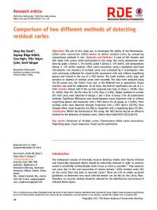
INTRODUCTION The Von Kleinsmid Center (VKC – see Figure 1) is a landmark building at the University of Southern California in Los Angeles, CA. Built in 1966, it has a non-occupied prominent brick tower and three-story brick blocks in a U-shape distribution around a central exterior courtyard. The courtyard has an amphitheater in the lower level. On the ground level, it contains covered arcades used mainly for circulation and some sitting places with landscaping. There are no close neighboring buildings obstructing solar access and only a few trees to the southeast and northwest. The total area of 95,287 sft (8,852 m2) is distributed in a library in the basement, classrooms in first and second floors, and offices in the upper floors. Design Builder 3.0.0.091 and eQuest 3-64 were used to model this building. They use Energy Plus and DOE2.2 respectively as their energy simulation engines. They were chosen because they are widely used by practicioners and academics. The methodology consisted of data collection, on-site measurements, simulation, and analysis of the results. In parallel, experiments were run to study issues detected in the process of simulating the building. Throughout the

process, the main differences in modeling and simulating in the two software programs were observed and documented.

Figure 1. Von Kleinsmid Center (VKC)

SIMULATION AND EXPERIMENTS Simulations of the building in the two software tools required several stages to obtain the closest match between the digital results and the measured data. Weather data. Real weather data for 2010 was obtained for the closest weather station. It was from the KCQT weather station, latitude 34.0511 degrees north, 118.235 degrees west, in downtown Los Angeles. This is approximately three miles from USC. Both .epw and .bin files were obtained. According to that weather data, September 27st was the hottest day with a maximum temperature of 106.8°F at 5pm, and December 31st at 2pm the coldest with a temperature of 37.1°F. Winds are generally from the south west and west directions with wind temperatures varing from 32°F to 75°F. (Khuen, Ch. 2011) Building geometry. The building’s geometry was input into Design Builder and eQuest. This information came from the original

architectural drawings obtained from Facilities Management Services, USC. Both of the models simplified the colonade defining the central courtyard and the northeast facade. The site orientation, timezone, longitude and latitude were also entered.

The Revit file was exported as a gbXML file and then imported in Design Builder. Initially, it appeared that it was a complete waste of time to have created the model in Revit as none of the objects were transferred properly to Design Builder. However, a work-around was found; by transferring the model first to Ecotect then creating a gbXML file, the building model was able to go into Design Builder. However, many adjustments had to be made. All the punctures in the model in the form of windows and doors were verified and adjusted as needed. The cut out in the basement had to be totally remade in Ecotect. The extended solar shades at the roof level had to be reconstructed as well. In addition, even after the file was exported to Design Builder again, some windows were missing and had to be reconstructed.

Figure 2. Building model in Design Builder

Figure 3. Building model in eQuest

Building geometry in Design Builder. It was a difficult task creating the VKC model, especially since it is a large building. The original model, created in Revit Architecture, was kept very simple in terms of massing and consisted of only the major exterior walls and no interior partitions. This was done after previous failures due to incompatibility issues between Revit and Design Builder. Special care was taken to verify that all the walls touched the roof in Revit model, or else when exported in simulation software the “zone” is not properly recognized leading to error in simulation. “Rooms” (enclosed spaces in Revit) were added to the layout and named before exporting.

Figure 4. Revit model of VKC

Figure 5. Ecotect model of VKC

Once minor modifications were made, the internal partition walls were created in Design Builder. Overall, the transfer of the gbXML file from Revit to Design Builder through Ecotect was not clean but much better than a direct conversion to Design Builder. Building geometry in eQuest model. Simple profiles in the drawing file (dwg) were imported as references, and the entire geometry was redone. Those profiles also contained the definition of different zones in the building. The possibility of importing a .gbXML file was explored, but eliminated due to the complexity of the conversion to make it readable in the software. Facades were matched exactly to the original drawings. This means that all windows and doors were modeled with real dimensions from original drawings. Building features. Walls (sub-grade and exposed), slabs (sub-grade and internal), roof, and finishing materials have been matched using the exact U-values and dimensions in both software programs. The glass properties like visible light transmittance, U-value, and SHGC were also entered in both eQuest and Design Builder.

The roof is flat aggregate and covered with an asphalt application. The structure of the building, which is finished with the brick veneer, is reinforced concrete and steel. Interior partitions are painted sheetrock walls distributed in a grid of concrete columns. Floor finishes vary among spaces, with vinyl in the library and classrooms and carpet in the offices. Ceilings are a combination of acoustical tile and textured sheetrock. Zoning, use, and schedules. The building’s basic functions are library space, classrooms, and offices. Unconditioned areas account for 11% of the total area of the building and are mechanical rooms, restrooms, and access areas. The library is located in the underground area where daylighting is provided by the central courtyard through a fully glazed perimeter. Classrooms are located in the east and west blocks and are of two types, old traditional and new classrooms. The latter have been equipped with modern controls for occupancy and equipment, which resulted in different schedules. Offices are located in the second floor of the north block and the entire third floor. There are two computer labs, located on the second floor and third floor. All schedules for occupancy, lighting, and equipment were matched in both models. The occupancy schedule was obtained from the classroom scheduling office at USC. Equipment usage within the class is not directly proportional to the number of classes and their duration. Not all classes use the audiovisual equipment. A recorded list of equipment usage was obtained from Information Technology Services (ITS) department at USC. This department keeps a log when the equipment is used and for what classes. This was helpful to determine the intermittent load for classrooms, which formulates to the majority of classroom equipment load. The HVAC schedule was obtained from Facilities Management Services at USC for both school year and summer hours of operation. HVAC. Currently, the building is conditioned with four air handling units (AHU). Infrastructure steam feeds a heat exchanger that generates hot water for heating. Steam condensate is handled by one central accumulator/return system. Hot water is circulated to air handler coils for preheat and primary heat. Hot water is also circulated to reheat terminals. Over more than forty years of use, the original HVAC distribution has migrated to a variable volume design. The original constant volume duct and air control dampers remain in service and are not optimal for a

variable air volume design, which would ideally be medium pressure design. The air handler, valve, and local controls are mostly pneumatic in design, but direct digital controls (DDC) has been incorporated over time.

Figure 6: HVAC zoning of the building

Representing the modified systems over time is one of the main challenges simulating exisitng buildings. In this study, the system supplying the basement floor was kept as multizone constant volume system, while the rest of the systems were converted to behave as variable volume.

DISCUSSION & RESULT ANALYSIS This section is divided in two parts. First, the theoretical differences of both simulation software programs are discussed, following which the limitations and results are described. 1. Theoretical Comparison These differences are important to understand the functionality of each software tool. This in turn leads to different calculations parameters that could explain different simulation results. Calculation Method  Design Builder: thermal balance method  eQuest: weighing factor method Calculation Time  Design Builder: depends on complexity set on model. It can take much more time compared to eQuest.  eQuest: faster (quick) Temperature  Both eQuest and Design Builder have only one user defined temperature per zone.

Load Calculations Design Builder uses an integrated simulation methodology that solves for heat and mass balance for each surface and calculates space loads and building systems simulation at the same time step. “Zone,” “system,” and “plant” talk and provide feedback to each other for each time step of simulation. In this case, an energy balance equation is written for each enclosing surface in addition to an equation for room air that allows the net instantaneous sensible load to be calculated for space air. (Wadell and Kaserekar 2010) Non-linear processes like air convection, solar gain, and radiation from interior surfaces are taken into account as the net energy transfer to each inside surface. This energy must be exactly balanced by heat conducted to or from those surfaces. This resulting variable surface and air temperatures are solved by energy balance equations leading to net heating and cooling loads for the zone. On the other hand eQuest assumes that all processes modeled are independent of each other and linear in operation. Heat gains are calculated independently from various sources and then added together to obtain the total cooling load. (Hunn 1996) While calculating the load, instantaneous heat gains for the zone are calculated using the fixed user specified zone temperature. Non-linear processes like convection or radiation are approximated linearly. Transfer coefficients are constant, and no dynamic heat flow is calculated. In the case of solar gains, eQuest uses a user-defined fraction multiplier for all opaque objects and interior surfaces to calculate the incident direct and diffused solar radiation in the space. By default, 60% is absorbed by the floor and the remaining 40% is distributed to the remaining surfaces based on their areas. Once the cooling load is calculated, weighting factors are applied to the zone materials to estimate the energy stored that would be released later to the space. Only one set of weighting factors is used over the entire simulation period. (Hunn 1996, Wadell and Kaserekar 2010)

Design Conditions Design Builder has preset ASHRAE Handbook recommended outside dry bulb and wet bulb temperatures required to calculate heating (99.6% and 99% coverage) and cooling loads (99.6%, 99%, 98% coverage) for all locations in the Design Building location template. It even has a typical dry bulb range that it uses to calculate hourly dry bulb temperatures for the 24 hour design period. While calculating cooling loads, Design Builder gives an option of choosing the design month and date to be a design day. However,

Design Builder does not use outside dry bulb (ODB) and outside wet bulb (OWB) temperatures of that date and month from the weather file but uses ASHRAE defined outside temperature to calculate the load. The schedules of the chosen design day are also not followed to calculate the load. Summer and winter day design schedules are described clearly while making the schedule for each function in building. While calculating loads, Design Builder just uses its own schedule irrespective of the fact that design day chosen might be a holiday or a weekend. The only way that loads get affected by choosing different design days or months is due to radiant transfer of heat. Different amounts of solar gains get transferred inside the space either directly through windows or by radiant fraction from the walls because of the different solar angles in different months. Solar gains through windows, roof, and ground are the main contributors to this. eQuest gives two options to the user. Either the user can define the design days based on ASHRAE Handbook data to help eQuest determine the peak loads for system sizing, or eQuest will automatically calculate peak loads and size HVAC systems using the weather file. If using the user defined data, the design day input tab needs to be in the project component tree which results later on in the generation of design day report (LS-A space peak load summary report) within the D2SIM. eQuest provides an opportunity to either set one day as the design day or set the range of days out of which eQuest can calculate peak loads and size the system while using user-input design day option.

Sizing of Systems Design Builder uses algebraic energy and mass balance equations combined with steady state component models to simulate HVAC systems. It provides four options for calculating loads and sizing systems. These options are ASHRAE, variable air volume (VAV), fan coil unit (FCU) and unitary DX. These four options do not have much impact on sensible cooling requirement of the space, but they do affect design flow CFM required and latent cooling. These parameters collectively lead to different cooling loads. As a methodology, peak loads and moving averages for the system are calculated using zone sizing and outside weather conditions for each sizing period. Then the system sizing calculations are performed. On the other hand, eQuest does not give any type of Design Builder options, but does give an option to calculate loads based on coincident or non-coincident parameters. According to coincident parameter, supplyflow is sized using the peak value of sum of loads of the

zones on the system (Hirsch J. 2010). However, noncoincident parameter sizes the supply-flow using the sum of peak loads of the individual zones.

2. Limitations and Results The process of calibrating the building in two software programs presented the following issues: limitations in modeling the basement floor consistently, calculation of areas, weather files, and peak load calculations. Limitations in Modeling: Geometry of Basement The geometry of a floor with a central courtyard was limited by the capabilities of eQuest to create footprint shapes as a “shell.” EQuest creates a shell based on only one closed polyline. In other words, a shell could not be created with a second polyline that could then be subtracted as a void space to resemble the open space courtyard. This was also confirmed by verifying with the “rectangular atrium” footprint shape template contained in eQuest. Therefore, the basement walls followed the original profile except for two segments of the polyline (two internal walls) that connected the rectangular atrium with the outer walls. That connection was determined in the thinnest section of the floor to minimize the impact of those walls. These walls were adiabatic in nature. However, no such problem was encountered in Design Builder. The courtyard geometry could be easily constructed or imported from Ecotect/Revit via gbXML.

Limitations in Modeling: Adjacency of Basement Even though eQuest capabilities for underground construction are very straightforward, it does not allow the creation of an open-air central courtyard below grade. The method described above allowed modeling the geometry with a central courtyard but the central void was being treated as ground and not as open space. The openings could not be modeled on the courtyard facing walls as the adjacency was modeled as ground conditions and not as exterior wall. On the other hand, Design Builder could courtyard facing basement walls as exterior changing the adjacency of those walls. openings in the form of full floor glazing easily modeled.

treat the walls by All the could be

In order to resemble the actual conditions in eQuest, it was decided to lift the whole building to create a first floor instead of a basement and give higher R-Values with high thickness of concrete to the outside perimeter walls in order to replicate the ground conditions.

Calculation of Areas A discrepancy of 5% – 7% was found in light and plug load consumption as predicted by Design Builder and eQuest. All the lighting power densities (LPD) and equipment power densities (EPD) for all zones were verified within both Design Builder and eQuest. Schedules were also verified again, but no flaws were found. Two conjectures were proposed as to why both software programs showed the same difference in the calibrated models: eQuest predicts higher levels than Design Builder with same inputs and/or something was neglected in the input section. An experimental model was made with a 30’ x 30’ square plan with all walls’ thicknesses as 6” in both Design Builder and eQuest. All inputs were input exactly the same in both software programs. Both the LPD and EPD were kept at 1 W/sft. Upon running the annual simulation, there was still about 7% difference between the electrical consumption by light and equipment end use. However, as the LPD and EPD were kept same as an input, both models predicted the same consumption of electricity for light and equipment, but with the constant difference of 7%. The reason for this difference, in light and plug load consumption, was finally tracked down to the “areas” of the experimental models. It was determined that even if the model was made using the same dimensions, the areas of the two were still different. Design Builder used those dimensions as an external boundary dimensions and deducted the external wall thicknesses from the plan reducing the floor area. However, eQuest treated it as an internal zone space and kept the full area as conditioned floor area. This difference led to the decrease in electrical consumption from lights and equipment as they were specified as watts consumed per square foot (W/sft) in the input screen. Design Builder having less area, had less electrical consumption as compared to eQuest resulting in the 7% difference. Once the area was matched between the two programs, the electrical consumption by both light and equipment end uses also exactly matched. This understanding of problems in area calculations was then used to understand the difference in the VKC simulation model. It was realized that 4.6% of the total footprint was used in the walls. Upon taking an estimated LPD and EPD for the whole space and multiplied by this additional 4.6% of area, the mystery seemed to be solved. The lighting end use difference reduced from 5% to 1.2% whereas equipment end use difference reduced from 7% to 2%.

Design Conditions: Weather File ASHRAE 99.6% coverage defined ODB, OWB, and design day for Los Angeles was used to calculate the peak loads in the building. This information could be easily selected in Design Builder as it exists as a template. The schedules for design day were defined as a typical weekday based on different functions in the building. However when these design conditions were to be specified in eQuest, it was realized that there was no tab to enter this data. The cooling and heating design tabs in the eQuest component tree that allowed user based parameters were absent. This was a mystery, and it was realized that load calculations only reported loads in the standard report whereas the design day report was absent. This meant that eQuest was calculating the design loads based only on the weather file and not on the ASHRAE defined parameters. The actual 2010 measured weather was used in eQuest in the wizard mode initial model. In order to solve the mystery, the first step considered reviewing the weather file and looking for clues that indicate the existence of those design days within some section of the data. After opening the weather file, it was noticed that the file did not contain any header section. In traditional .epw files, location, geographical coordinates, heating, and cooling design day information are contained in the header. This was a major lead in solving the mystery. However, the header was to be created in the VKC weather file in order to make cooling and heating design tabs reappear in the component tree. In order to get the header information, Los Angeles International Airport weather file (.epw) was examined. The header was extracted from this file and added to the VKC weather file. (Note: .epw files can be modified and saved in a text editor, but “all files” must be selected as type). This new .epw file was then converted to .bin file using the eQuest weather processor without any errors or warnings. This seemed to have solved the problem. However, when the simulation was run again using the new .bin file, the anticipate design day tabs were still not found. As a second step, a small experiment was performed using the already contained locations predefined in eQuest. Basically, the software contains California zones, on-line linked options in addition to those that are user defined. The locations that are on-line linked had the same problem generating design day options. Only the locations linked to California climatic zones were able to generate the sections for design day calculation in the component tree and consequently the detailed report. The test used Los Angeles (associated with California Zone 6-CZ06), and the cooling design

day and heating design day components were created on the tree. This clarified that it was not only VKC weather file that did not generate these design day components but all the weather files except that of default California zone climate files. In other words, it was only California Zone climate files that could allow later to calculate ASHRAE based design day peak loads, and the other weather files calculated loads based on weather data. However, the California zone climate file couldn’t be used as the weather file for the calibration purpose. The VKC weather file was modified incorporating the missing header from the California Climate Zone weather file. This strategy also did not work as the cooling and heating design day tabs did not appear in the component tree. This meant that the information for design days was not contained only in the header. A small experiment was run using CZ06 climate data. The description for both cooling and heating design day was extracted from its .inp file and incorporated in VKC .inp file. This finally worked and the design day tabs were finally visible in component tree. To understand the difference between CZ06 and LA International Airport (LAX) based weather files (.bin), it was desirable to explore inside the file. However, the .bin file could not be opened successfully in an appropriate manner in order to assess the difference between the two. This missing header in the VKC file did not give any problems in Design Builder as it does not require design day information from the weather file. The tabs and design day information are already defined based on ASHRAE separately from the weather file. Peak Load Calculations for Sizing Because the inherent differences in choosing design days determining peak loads and sizing systems (see Design Conditions Sizing of Systems above) the same system sizes were manually inserted in both models.Therefore, the same loads were expected. However, that did not prove to be the case. During the initial comparison, there was very high percentage difference between cooling and heating loads calculated by Design Builder and eQuest. Design Builder predicted 37% more for peak cooling loads and 55% more for peak heating loads. This difference could either be because of the difference in the calculation methodology between two softwares discussed earlier or because of something that was overlooked. Looking at the vast percentage difference, the latter case sounded reasonable.

After some investigation work, it was discovered that there is a difference in the way loads are calculated by Design Builder and eQuest. Design Builder simply adds the loads from all the zones to give the total load. However, eQuest gives the load for all zones and also for the full Building Peak load at the worst hour. Building peak load is always less than sum of loads in all zones, because the zone peaks do not all occur at the same time. Initially the comparison made was between Design Builder combined peak loads versus eQuest building peak load that resulted in a big difference. It was best suited to compare combined loads from all zones for comparing the two software in order to have a common platform. Even if combined loads of all spaces were compared, there was still some discrepancy. Peak cooling loads were quite close with only 1.8% difference (being eQuest higher) but still heating loads were predicted by Design Builder 18% more than eQuest. No possible reasonable explation was found. An in depth study was done to unravel this mystery. A manual spreadsheet was created for calculating heat loss through the VKC envelope and compared against eQuest and Design Builder predicted values. The heat loss was compared for each component of the envelope in order to access the difference. During this process, another difference between the way eQuest and Design Builder calculates peak heating load was discovered. In order to calculate the load for a zone, eQuest takes into account equipment, light, and occupancy gains which is not considered by Design Builder. This meant the Design Builder predicted loads should be less than eQuest. Infiltration and external ventilation values were kept as zero for simplification purpose. Table 1: Heat loss calculations Heat Loss By Component (kBtu/hr) ‐ VKC Manual Calcs DB % Diff eQuest Walls 268.6 223 17% 176 Roof 276.2 215 22% 316 Windows 233.3 140 40% 260 Basement Floor 109.2 54 51% 15 0 External Ventilation 0 0 0 Infiltration 0 0 Total Heat Loss 887.2 632 29% 767

% Diff 34% ‐14% ‐11% 86%

14%

EQuest and Design Builder predicted peak loads were 14% and 29% respectively lower than manually calculated heat loss. There were further differences in individual building loss components. Sizing of HVAC In order to calibrate the energy model to the actual building, HVAC systems were not autosized but the exact description was input manually. The CFM at air

handling units were noted from the air balance report and put in acurately in both simulation softwares with the same efficiency and pressure rise of fans. The fan curve was matched within both softwares. Economizer control type was selected to be differential enthalpy with outdoor dry bulb temperature low limit as 50 and high limit as 70. There are two chillers (same model) in VKC. Part load curves were obtained from Trane for that specific chiller model, and the same co-efficients were inserted in both software. The detailed hourly amps, supply temperature, and return temperature values were obtained from Facilities Management Services, USC. The power consumption of the chiller was calculated based on this information and compared to the power consumption estimated by both simulation softwares. The controls of both chiller were kept sequential as in the VKC. The chilled water pump, condenser pump, and boiler pump were exactly matched for flow rates, power consumption and head. All pumps were set to constant speed but intermittent control type. These exact matching of HVAC systems helped in calibrating the model. A comparison of calibrated results between both softwares are discussed below.

ANNUAL SIMULATION RESULTS Energy predictions for VKC building in both software programs are discussed for electricity, gas, and end uses. Both software programs predictions for annual electricity were less than the real annual energy use of the building. According to ASHRAE 14 a simulation model is set to be calibrated if the error margin is within ±15% as per Cumulative Variation of Root Mean Squared Error (CVRMSE). Annual energy consumption predicted by Design Builder and eQuest was 17% and 9% error margin respectively. However, annual gas predicted by both Design Builder and eQuest was far less than the real annual consumption in the building. The percentage difference was 98% and 80% for Design Builder and eQuest respectively. It is highly probable that the “real” data from the building is erroneous. After discussing the matter with facility management services at USC it was realized that there was not proper way of measurement of gas consumption at VKC. Gas was measured with a common meter shared by four buildings. The gas usage was then allocated to all four buildings based on

assumptions. Consequently no further calibration was pursuit for gas consumption.

CONCLUSION Two energy simulation programs, Design Builder and eQuest, were used for modeling the same institutional building. Both models used the same measured energy data and actual weather file for a specific year. These energy software programs used different calculation techniques and methodology that resulted in different predictions. During the process, both software programs presented different limitations while calibrating the building. Even after matching all the inputs, the loads calculated by both software programs were different. However, annual predictions were comparatively closer in terms of amount, profile, and end uses.

ACKNOWLEDGEMENTS Doug Avery at Southern California Edison (partial funding); Chuck Khuen for providing weather data files.; and Carol Fern at the University of Southern California Facilities Department. Fig.7. VKC real electricity use and monthly predictions

End Uses Recorded end uses fit quite well with end-use predictions by both software programs. Respectively, Design Builder and eQuest predicted similar values (KBtu/sf/yr) for plug-loads (9.9 and 10.8) and lighting (13.3 and 11.8). However the predictions for chillers (6.6 and 12.3), fans (3.5 and 5.5) were lower in Design Builder. These end uses lead to the lower annual prediction given by Design Builder.

Fig.8. VKC end uses for both Design Builder and eQuest

REFERENCES ASHRAE Handbook, 2005. ASHRAE Fundamentals. Hirsch J.J.& Associates. DOE-2 Documentation, V.2.2, September 2001.Volume 3, Topics. Simualtion Research Group, LBNL Hunn, B. 1996. Fundamentals of building energy dynamics. MIT Press. Khuen, Ch. 2011. Weather Analytics. Available at www.weatheranalytics.com [Accessed on 2011] J.S.Haberl, T.E. Bou-Sada, “Procedures for calibrating hourly simulation models to measured building energy and environment data,” ASME Journal of Solar Energy Engineering 120 (1998) 193-234. Raftery, P. Keane, M., Donnell, J. “Calibrating whole building energy models: An evidence-based methodology,” Energy and Buildings 43 (2011) 36663679. Pan, Y. Huang, Z. Wu, G. “Calibrated building energy simulation and its application in a high rise commercial building in Shanghai,” Energy and Buildings 39 (2007) 651-657. International Performance Measurement & Verification Protocol Committee. 2002 Volumen 1. Available at http://www.nrel.gov/docs/fy02osti/31505.pdf. Accessed February 2012. U.S. Department of Energy Federal Energy Management Program M&V Guidelines: Measurement and Verification for Federal Energy Projects Version 3.0. Available at http://www1.eere.energy.gov/femp/pdfs/mv_guidelines.p df. Accessed February 2012. Waddell, C., Kaserekar, S. 2010. Solar gain and cooling load comparison using energy modeling software. SimBuild.