Comparisons of Packet Scheduling Algorithms for Fair Service among ...

Comparisons of Packet Scheduling Algorithms for Fair Service among Connections on the Internet Go Hasegawa, Takahiro Matsuo, Masayuki Murata and Hideo Miyahara Department of Infomatics and Mathematical Science Graduate School of Engineering Science, Osaka University 1-3, Machikaneyama, Toyonaka, Osaka 560-8531, Japan Phone: +81-6-850-6616, Fax: +81-6-850-6589 E-mail: {hasegawa,t-matuo,murata,miyahara}@ics.es.osaka-u.ac.jp February 23, 2001

Abstract

1

Introduction

We investigate the performance of TCP under three The conventional Internet has only been providing representatives of packet scheduling algorithms at the best effort service, and it could not offer throughthe router. Our main focus is to investigate how fair put and/or delay guarantees. It is also lack of fairservice can be provided for elastic applications shar- ness guarantees; TCP connections sometimes receive ing the link. Packet scheduling algorithms that we unfair performance in terms of, e.g., throughput. consider are FIFO (First In First Out), RED (Ran- See, e.g., [1]. However, we now need to provide dom Early Detection), and DRR (Deficit Round Robin). commercial network services by the Internet. That Through simulation and analysis results, we discuss is, a new service should be available within the netthe degree of achieved fairness in those scheduling work to support the differentiated services among algorithms. Furthermore, we propose a new algo- the users [2]. Along with the context of diff-serv rithm which combines RED and DRR algorithms models, several service principles have recently been in order to prevent the unfairness property of the proposed; for example, a constant throughput may original DRR algorithm, which appears in some cir- be preferred to some connections, or QoS support is cumstances where we want to resolve the scalability necessary for real–time applications. For example, problem of the DRR algorithm. In addition to TCP in [3], the authors have proposed an Explicit CapacReno version, we consider TCP Vegas to investi- ity framework for allocating the network capacity gate its capability of providing the fairness. The re- to users in a controlled way even during congestion sults show that the principle of TCP Vegas conforms periods. to DRR, but it cannot help improving the fairness Another important service that the next–generation among connections in FIFO and RED cases, which Internet should support is fair allocation of the bandseems to be a substantial obstacle for the deploy- width, which is our main subject of this paper. It is ment of TCP Vegas. one of most desired features for elastic applications, keywords: Fairness, FIFO (First In First Out), but not supported by the current Internet, and we beRED (Random Early Detection), DRR (Deficit Round lieve that it may be more important even than netRobin), TCP (Transmission Control Protocol) work efficiency. A one existing service found in the

1

literature is the USD (User Share Differentiation) scheme described in [4], where users are provided different service qualities from ISPs (Internet Service Providers) based on the contracts. However, the authors in [4] do not provide a quantitative evaluation of USD to show how the users are differentiated. One promising way to realize the service differentiation for the elastic applications seems to be DRR (Deficit Round Robin) presented in [5] where the round robin scheduling is performed among active connections. In [5], an extensive evaluation of the DRR algorithm is provided, but they assume Poisson arrivals of packets from each connection. That is, the authors do not consider the behavior of the upper–layer protocol, i.e., TCP (Transmission Control Protocol). In this paper, we focus on the degree of fairness provided to TCP connections by comparing three packet scheduling algorithms at the router. The first one is FIFO (First In First Out, or Drop–Tail), which is widely used in the current Internet routers because of its simplicity. The second is RED (Random Early Detection) [6], which drops incoming packets at a certain probability. While the original idea of the RED algorithm is to avoid consecutive dropping of packets belonging to the same connection, it also has a capability of achieving a fair service among connections by spreading packet losses. The last one is DRR, which is a more aggressive one in the sense that it actively maintains per–flow queueing for establishing fair service. For TCP, we consider the Reno version, which has widely been used in the current Internet. The Vegas version [7], adopting a different congestion control mechanism from TCP Reno for larger performance gain, is also considered. In this paper, for reference purposes, we will first show simulation results that FIFO cannot provide fairness among connections at all because of a bursty nature of packet losses (see Subsection 3.1). It is next shown that RED offers better fairness than FIFO to TCP Reno connections, but it cannot keep a good fairness when the capacity of shared link becomes small compared with the total input link capacity (Subsection 3.2). In TCP Vegas, on the other

hand, RED offers less fairness than FIFO because of the essential incompatibility of TCP Vegas to the RED algorithm (Section 4). The packet scheduling algorithms and TCP versions that we will use in this paper are not new. Our main contributions in the current paper is that the properties mentioned above are also shown through analytical results. While the model used in the analysis is very simple, the basic features of the above scheduling algorithms can be well explained. From the analysis results, we further propose the enhanced version of RED algorithm, where we set each connection’s packet dropping probability dependently on its input link capacity, to avoid the unfairness property of the original RED algorithm. Another enhancement method of RED can be found in [8], where the flow state are maintained for some degree of fairness enhancements. The above method can be used to resolve an inherent problem of the DRR algorithm. DRR can provide almost perfect fairness among connections in both cases of TCP Reno (Subsection 3.3) and Vegas (Subsection 4.3), but DRR requires per–flow queueing. Since we mainly consider the ISP model, we may not need to consider the stateless fair queueing mechanism such as the one found in [9]. However, DRR has a scalability problem in that as the number of subscribers grows, the larger number of queues becomes necessary. One possible solution is flow aggregation which treats several connections as a single flow of DRR. However, it results in that the fairness property of DRR becomes lost when multiple TCP connections are assigned to the same queue. Based on our analytical results, we last apply the RED mechanism to each queue of DRR (called DRR+) for fairness enhancement. We show that our DRR+ can provide a reasonably good fairness even compared with DRR through the simulation results (Subsection 3.4). In the above discussions, we use the network model where the uplink of the access line of ISP is shared by the subscribers with different capacities. In this paper, the effect of the reverse traffic is also considered. in the model where the downlink is shared by the subscribers. The objective of

this investigation is to confirm the applicability of our discussions and analyses in the above are also applicable to this reverse traffic model. The similar model is treated in in [10], but we consider RED and DRR as the packet scheduling algorithm in addition to FIFO algorithm employed in [10]. Further, we devote the fairness aspects of packet scheduling algorithms which are not considered in [10]. This paper is organized as follows. In Section 2, we describe the model treated in Section 3 and 4. The packet scheduling algorithms is first summarized in Subsection 2.1. We will also explain the congestion control algorithm of TCP Reno and TCP Vegas by focusing on those congestion avoidance mechanisms in Subsection 2.2. In Subsection 2.3, we explain the network model we will use in analysis and simulation, and introduce the fairness measure considered in this paper in Subsection 2.4. In Section 3, we evaluate the packet scheduling algorithms described in Section 2.1 in the case of TCP Reno through the simulation and the analysis, and propose DRR+ for fairness improvement. We next consider the case of TCP Vegas in Section 3. In Section 5, we investigate the effect of the reverse traffic flow. Finally, we present some concluding remarks and future works in Section 6.

The problem mentioned above is solved by RED [6]. The RED algorithm is designed to cooperate with congestion control mechanisms provided in TCP. In RED, the router observes the avarage queue size (buffer occupancy), and the packets arriving at the router are dropped with a certain probability. The DRR algorithm [5] is an extension of the round robin algorithm to be suitable to treat the variable– sized packets. The buffer at the router is logically divided into multiple queues. The arriving packets of each connection are stored in the pre-assigned queue by using a hash function, and those are served in a round–robin fashion. A difference from the pure round robin algorithm is that the packets with variable length can be allowed to keep the fairness among connections. In DRR, the bandwidth not used in the round is preserved to be used in the next round if the packet is too large to be served in the current round.

2.2

Congestion Control Mechanisms of TCP

In this paper, we consider two versions of TCP; Reno and Vegas. TCP Reno is widely used in the current Internet. TCP Vegas is a recently proposed one in [7]. In TCP Reno, the window size cwnd (conges2 The Model tion window size) is cyclically changed. cwnd continues to be increased until segment loss occurs. TCP 2.1 Packet Scheduling Algorithms Reno has two phases in increasing cwnd; Slow Start In what follows, we briefly summarize the three packetPhase and Congestion Avoidance Phase. When an scheduling algorithms, FIFO, RED and DRR for the ACK segment is received by TCP at the server side at time t + tA [sec], cwnd(t + tA) is updated from current paper to be self–contained. A FIFO algorithm is widely used in the current cwnd(t) as follows (see, e.g., [11]); Internet routers because of its simple implementacwnd(t + tA) = tion. The incoming packets are accepted in order   if cwnd(t) < ssth;  cwnd(t) + 1, of arrivals. When the buffer at the router becomes 1 (1) full, arriving packets are dropped. Therefore, pack , if cwnd(t) ≥ ssth;  cwnd(t) + cwnd(t) ets belonging to a particular connection can sometimes suffer from bursty packet losses. Then, fast where ssth [segments] is the threshold value at which retransmit [11] implemented in TCP does not work TCP changes its phase from Slow Start Phase to effectively. It is also likely to introduce bursty transCongestion Avoidance Phase. When segment loss mission of packets [6], which often results in further is detected by timeout or fast retransmission algopacket losses.

rithm [11], cwnd(t) and ssth are updated as

2.3

Network Model

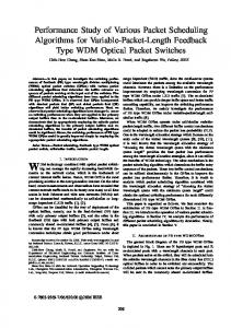
Recalling that our main purpose of the current paper is to investigate the fairness aspect of packet In TCP Reno (and the older version Tahoe), the scheduling algorithms, we will use a simple netwindow size, cwnd, continues to be increased un- work model as depicted in Figure 1. There are the number N of connections between til segment loss occurs due to congestion. Then, the window size is throttled, which leads to the through- N sources (SES1, SES2 , . . ., SESN ) and one desput degradation of the connection. However, it can- tination (DES). N connections share the bottleneck not be avoided because of an essential nature of output link of the router. The capacity of the inthe congestion control mechanism adopted in TCP put link between the sources and the router are deReno. That is, it can detect network congestion only fined as bw1 , bw2 , . . ., bwN Kbps, and that of the by segment loss. However, throttling the window output link between the router and destination is size is not adequate when the TCP connection itself BW Kbps. We assume bw1 ≤ bw2 ≤ . . . ≤ bwN . causes the congestion because of its too large win- By the above model, we intend to consider the updow size. If cwnd is appropriately controlled such link of the access line of the ISP, which is shared by that the segment loss does not occur in the network, the subscribers with different capacities. Note that the throughput degradation due to the throttled win- in Section 5, we will consider the downlink of the dow can be avoided. This is the reason that TCP access line. In the following numerical examples throughout Vegas was introduced. TCP Vegas employs another mechanism, in which the paper, the propagation delay between SESi and it controls cwnd by observing changes of RTTs (RoundDES, τ , is identically set to be 100 msec. The buffer Trip Time) of segments that the connection has sent size of the router is 60 Kbytes. A TCP packet size before. If observed RTTs become large, TCP Ve- is fixed at 2 Kbytes. Every sender is assumed to gas recognizes that the network begins to be con- be a greedy source, that is, it has infinite packets to gested, and throttles cwnd down. If RTTs become transmit. We also assume that in the case of DRR, small, on the other hand, TCP Vegas determines that the connection can be identified by the router so that the network is relieved from the congestion, and in- the packets from the connection can be appropricreases cwnd again. Then, cwnd in an ideal situ- ately queued at the per–flow buffer at the router. ation becomes converged to the appropriate value. In Congestion Avoidance Phase, the window size is 2.4 Definition of Fairness updated as; We define the fair service by taking account of the cwnd(t + tA ) = input link capacity. Its simplest form is that the  α throughput is given in proportion to its input link   cwnd(t) + 1, if diff < base rtt β α cwnd(t), if base rtt ≤ diff ≤ base rtt(2) capacity under the condition that the output link ca  pacity is smaller than total of the input link capacicwnd(t) − 1, if baseβ rtt < diff ties. That is, we say that a good fairness is achieved diff = cwnd(t)/base rtt − cwnd(t)/rtt if the throughput of connection i, ρi, is given as where rtt [sec] is an observed round trip time, base rtt [sec] bwi is the smallest value of observed RTTs, and α and ρi = BW ·  j bwj β are some constant values. Note that Eq. (2) used in TCP Vegas indicates that if RTTs of the segments We note that other definitions of the fairness can are stable, the window size remains unchanged. be considered. A more natural definition may be the ssth = cwnd(t)/2; cwnd(t) = ssth

function of subscription fees, which may be deter-

mined by (but not be proportional to) the input link capacity in the ISP model. We will not treat such a case for simplicity of presentation, but it is not difficult to incorporate it. For example, the weight factor is allowed to be arbitrary in the DRR case. The RED case can also be treated in this context by utilizing our analysis presented later.

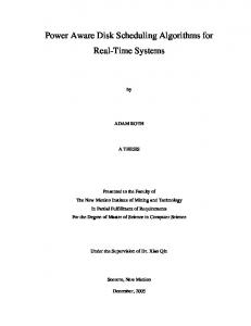
as follows. In the FIFO algorithm, packet loss occurs independently of the packet arrival rate as shown in Figure 2(c), and the packet loss becomes bursty. Since the connection with larger input link capacity experiences a higher degree of burstiness of packet losses, its performance degradation becomes larger.

3.2

3

The Case of TCP Reno

3.2.1

RED Case Simulation Results

We next investigate the RED case. Recalling that the buffer size of the router is set to be 60 Kbyte, we set thmin = 10 Kbytes, thmax = 30 Kbytes and p = 0.02 in simulation. p shows the packet dropping probability defined in RED, with which incoming packets are dropped when the avarage queue length is over the threshold thmin. Figure 3 shows simulation results of the RED algorithm in that case. From Figures 3(a) and 2(a), it can be observed that a fairness improvement is very limited. It is especially true when the output link capacity is small; the throughput of all connections becomes almost identical (Figure 3(a)). Also, the packet loss rates of all connections are almost equal as shown in Figure 3(c). Of course, this is one of key features that the RED algorithm intends; the number of the lost packets of each connection can be kept in proportion to its input link capacity by its mechanism. The problem is that it leads to the unfairness treatment 3.1 FIFO Case of connections with different capacities. The above result is just one example. Also, it We first show the FIFO case in terms of the avis questionable whether simulation time of 300,000 erage throughput during the simulation run (Figure 2(a)), the relative throughput (Figure 2(b)), and packets generation is adequate or not for examinpacket loss rate (Figure 2(c)) for all connections as a ing the fairness degree. To examine its generality, function of the output link capacity. Relative through- we next show the analysis of the RED algorithm. put means the ratio of the average throughput against Through analysis, it is proven that the unfairness the input link capacity. When all connections have observed in simulation is inherent in the RED alidentical relative throughput, it is said that the router gorithm. We assume in the following analysis that there perfectly provides fair service among connections are N connections in the network (Figure 1) with in our definition. From Figures 2(a) and 2(b), it is clear that fairness cannot be kept at all. In some the input link capacities of bw1 , bw2 , ..., bwN [packregion where the output link capacity is small, the ets/sec], where bw1 ≤ bw2 ≤, ..., ≤bwN . We dethroughput of the connection with smaller input link note the packet dropping probability of the RED alcapacity is larger even than that of the connection gorithm by p, and the propagation delay between with larger input link capacity. It can be explained sources and the destination by τ . We also assume In this section, we consider TCP Reno to investigate the fairness property of three packet scheduling algorithms. In addition to the simulation results, we develop the analysis result for the RED scheduling algorithm. The analysis results supports observations on the fairness property of the RED algorithm obtained from the simulation results. We then investigate DRR to demonstrate its effectiveness through simulation experiments. In what follows, we set four TCP connections which have different capacities of 64, 128, 256 and 512 Kbps. The output link capacity is varied from 400 Kbps to 960 Kbps to investigate the effect of the output link capacity on fairness. In the simulation results, we simulated 5,000 sec in each experiment to obtain the result, which approximately corresponds to 300,000 packet generation.

that the average queue length is always larger than and Wmax . That is, thmin , that is, all arriving packets are dropped with  8 probability p. For analysis, we focus on TCP’s typW max  (7) 3p ical cycle of the window size as shown in Figure 8; the cycle begins at the time when the previous packet As a result, we derive Wa [packets], the average loss occurs, and terminates when the next packet window size during the cycle as; loss occurs. We consider that the cycle begins at time t = 0 [sec]. We do not take account of the slow 3 W max (8) Wa = start phase [11] since the objective of the RED algo4 rithm is essentially to avoid to fall into that phase. Since all arriving packets are dropped at the router See Figure 8. From the equation above, we can see with probability p by our assumption, the connec- that the change of the window size does not depend tion can send 1/p packets in one cycle (between the on each connection’s input link capacity, but on the events of packet losses). We define the number of packet dropping probability of the RED algorithm. For further analysis, we make an assumption that packets transmitted during one cycle as Np , that is, each connection’s window size is fixed at the aver(3) age value, Wa. We then derive ρi , the throughput Np = 1/p. of connection i when Wa packets of its window are During the cycle, the window size of connection i, served at the router. To simplify the analysis, we cwndi (t) [packets], is increased linearly since we consider the situation where all connections’ first only consider the congestion avoidance phase [11]. packets of the windows arrive at the router simulThe window size is halved when packet loss de- taneously as shown in Figure 9. In this figure, each tected by fast retransmit, and therefore cwndi(t) is square shows the burst of connection i’s Wa seggiven as ments, and its length represents the time duration Wa bwi [sec]. Since all connections have different / Wmax 1 · t, 1 ≤ i ≤ N, (4) capacities bwi on their links, it takes different time cwndi (t) = + 2 RT Ti duration Wa/bwi for all packets of connection i to where RT Ti [sec] is an average round trip time of arrive at the router as illustrated in Figure 9. As packets for connection i, and Wmax [packets] is the illustrated in this figure, the segment burst of convalue of the window size at the time when packet nection i is not served at the same rate, and it deloss occurs. Then, the following equation for the pends on the number of the connections sending total number of the packets in one cycle should be their packets simultaneously. We divide all connections’ packet burst into N ‘phases’ according to the satisfied for connection i; number of connections which send the segments si Ti cwndi(t)dt = Np , 1 ≤ i ≤ N, (5) multaneously. For example, since the number of 0 connections which transmitting their segments is i in phase i, the router processes i connections’ segwhere Ti is the time duration of the cycle as shown ments at the rate of BW [segments/sec]. We denote in Figure 8. From Eqs.(4) and (5), we can obtain the number of packets of connection i belonging to
[packets], the window size at the time when Wmax phase j by Wi,j [packets] (1 ≤ i, j ≤ N). Since all the next packet loss occurs, as segements in the phase are dealt at the rate in pro portion to its input link bandwidth, we determine
= Wmax2 + 2Np (6) Wmax Wi,N for phase N as follows; From Eqs.(3) and (6), we can obtain W max [pack
ets], the average value of Wmax by equating Wmax

WN,N = Wa

Wi,N = WN,N ·

bwi , bwN

simple equation;

1 ≤ i ≤ N.

Pto =

In the same manner, we can obtain all of Wi,j by solving the following equations; Wj,j Wi,j

∞ i=2



Wa · pi · (1 − p)Wa +1−i (12) i

We assume that RT Oi [sec], the timeout duration for retransmission, becomes twice RT Ti , the Round = Wa − Wj,k , 1 ≤ j ≤ N − 1, Trip Time for connection i. RT Ti can be calculated k=j+1 by considering the effect of the other connections’ bwi = Wj,j · , 1 ≤ j ≤ N − 1, 1 ≤ i ≤ j − 1.traffic; bwj N



Wa The rate at which the packets are served at the router Wa k=i in the phase j, Sj [packets/sec], must depend on + RT Ti = 2τ + (13) BW ρi the total capacity of the connections of the phase j. Since, in the phase j, all packets belonging to from From these results, we finally have ρ
i , the throughconnection 1 to connection j are served at the router, put of connection i, by considering the effect of Sj becomes as follows; TCP’s retransmission timeouts;

Sj =

            

BW, j

j

if

bwk > BW ,

k=1

(9)

bwj , otherwise

ρ
i

= (1 − Pto ) · ρi + Pto · =

k=1

Wa ρi

ρi Wa + RT Oi ρi ρ2i · RT Oi

ρi · Wa + (1 − Pto ) · Wa + ρiRT Oi

(14)

Therefore, the throughput of connection i at phase j, Eq.(14) is obtained as follows. The first term (1 − Ri,j , can be determined as follows; Pto ) · ρi represents the throughput without retransRi,j =

j

Wi,j Wi,j

k=1

Wk,j

Sj

=

j

k=1 Wk,j

Sj

(10)

From Eqs.(9) and (10), ρi can be calculated as follows; ρi =

N k=N+1−i



Wi,j Ri,j Wa



(11)

Although the RED algorithm can eliminate the bursty packet losses leading to TCP’s retransmission timeout expiration, timeout expiration cannot be avoided perfectly [12]. Even if timeout expiration rarely happens, the effect of timeout expiration on throughput is large. Therefore, we next consider the throughput degradation caused by retransmission timeout expiration. We denote the probability of occurring timeout expiration in the window by Pto . We determine Pto according to the following

mission timeout, and the second term

Wa ρi

Wa ρi

+RT Oi

ρi

is that with retransmission timeout. By Eq. (14), we can obtain the each connection’s TCP throughput under RED algorithm with taking account of the througput degradation caused by TCP retransmission timeouts. Figure 10 shows the throughput results from our analysis as a function of the output link capacity. In the figure, points represent the simulation results (which correspond to Figure 3(a)), and the lines show analysis results. We can observe from this figure that our analysis can give good agreements with simulation results, and that the unfairness property of the RED algorithm in the case of small output link capacity can be observed. This unfairness can be explained from the analysis result as follows. When the output link bandwidth becomes small, the rate at which the packets are served at the router of phase j becomes BW in almost all the phases. It is clearly

shown in Eq. (9). That is, packets arriving at the Compared with Figure 3(b), it is clear that our enrouter are served at rate BW , which results in that hanced version of RED algorithm gives further betthe throughput of all connections become equiva- ter fairness than the original RED algorithm. In lent. Furthermore, the connection whose input link simulation, however, we set the control parameter bandwidth is larger can suffer from throughput degra- values of a and b intuitively. It is a future research dation caused by TCP retransmission timeouts. This topic to seek an appropriate method to determine is also the reason why the throughput of the con- those parameters. nection with the 512 [Kbyte/sec] input link bandwidth is largely degraded, which can be explained 3.3 DRR Case by Eq. (14). We next consider the enhancement to the RED As explained in Subsection 2.1, the router buffer is algorithm (called enhanced RED) to avoid this un- logically divided into several queues in DRR and fairness by setting p dependently on each connec- each connection is assigned its own queue. We first tion’s input link capacity, according to the analy- consider the case where the large buffer is equipped sis results. We set pi, which is the packet dropping with the router so that every connection is given a probability of connection i, such that each connec- sufficient amount of buffer. In our model depicted tion’s throughput becomes proportional to the its in- Figure 4, four DRR queues are formed in the router, put link capacity. The appropriate values pi’s are and DRR parameters are set such that each DRR calculated for all connections as follows. queue is served in proportion to the input link capacity of the assigned connection. 1. Initialize pi’s. Figure 5(a) shows the simulation results of relative throughput. Different from the FIFO (Fig2. Calculate ρi from the current pi according to ure 2) and RED (Figure 3) algorithms, the DRR althe analysis results. See Eq.(14). gorithm provides very good fairness among connec3. If ρi is proportional to the input link capacity, tions even when the output link capacity is small. set pi to the current value. When the output link is large, on the other hand, the degree of the fairness is slightly degraded. It is 4. If not, compare ρi with the ideal value, and because TCP’s retransmission timeouts tends to freadjust pi of the connection having the largest quently occur due to bursty packet loss at the queue difference between ρi and the ideal value. That since the FIFO discipline is used in each DRR queue. is, Then, the retransmission timeout degrades the per• If ρi is larger than the ideal value, change formance more seriously. Thus the degree of performance degradation depends on the bandwidth– pi to a pi . delay product of the connection. Furthermore, in • If ρi is smaller than the ideal value, change the DRR algorithm, the capacity not used by a cerpi to b pi . tain queue due to connection’s retransmission timeThe typical values of control parameters a and out can be used by other connections. It increases the total throughput, but it is likely to lead to the unb are 1.1 and 0.9. fairness among connections. This is why fairness is In the enhanced RED algorithm, we calculate the degraded in the case of the large output link. pi ’s for all connections from the connections’ input While the DRR algorithm assigns the DRR queues link capacities according to this algorithm, and set to each connection, several connections should be pi as the packet dropping probability at the RED assigned to one DRR queue as the number of conrouter in advance of starting to send the packets. nections grows. It is because the number of DRR Figure 11 shows the simulation results on the queues which can be prepared must be limited by relative throughput of the enhanced RED algorithm.

Figure 7 shows the simulation results on the relthe router buffer size and processing overhead. However, the performance of the DRR algorithm in such ative throughput. Our proposed method keeps good a case has not been known. For investigating such fairness in the sufficient buffer case (Figure 7(a)). an insufficient buffer case, we assume that there are Furthermore, when Figure 7(b) is compared with two queues and four connections, and each con- Figure 5(b), the fairness is significantly improved nection is assigned to the queue as shown in Fig- even in the insufficient buffer case. ure 6. The 64 Kbps and 128 Kbps connections are assigned to one queue (queue 1 in the figure) and the 256 Kbps and 512 Kbps connections to another 4 TCP Vegas Case queue (queue 2). Each queue is assumed to be served in proportion to the total capacity of the assigned In this section, we change the version of TCP to TCP Vegas to investigate the fairness property of connections. We show the simulation results in the insuffi- three packet scheduling algorithms. TCP vegas concient buffer case in Figure 5(b) for the relative through-jectures the available bandwidth for the connection, put. It is clear from this figure that the two con- and therefore its principle is likely to be well fit to nections assigned to the same queue show unfair the DRR algorithm. On the other hand, the RED throughput. This is because we assumed that the algorithm does not help improve the fairness when arriving packets are served according to a simple TCP Vegas is employed since each connection’s winFIFO discipline within the DRR queue. As described dow size is not dominated by the packet dropping in Subsection 3.1, the FIFO algorithm cannot keep probability of the RED algorithm, but by the essential algorithm of TCP Vegas. The purpose of this fairness among connection at all. In this subsection, we have observed that the section is to confirm the above observations. DRR algorithm gives much better fairness than FIFO and RED algorithms, but its fairness property is some- 4.1 FIFO Case times lost as each connection has different capacity or when multiple connections are assigned to one Figure 12 plots simulation results of the FIFO case DRR queue. We henceforth consider to improve the using TCP Vegas. Note that we omit the graph showfairness property of the DRR algorithm in the next ing the number of packet loss since no segment loss was observed at the FIFO buffer. Compared with subsection. the TCP Reno case (Figure 2), it is clear that TCP vegas provides less fairness than TCP Reno. Es3.4 DRR+ Case pecially, the connection with has smaller input link In the previous subsection, we have shown that the bandwidth achieve almost 100% throughput (FigDRR algorithm has some unfairness property. The ure 12(b)). This unfairness property is caused by main reason was that each DRR queue serves pack- the essential characteristic of TCP Vegas. In TCP ets by the FIFO discipline. In this subsection, we Vegas, no segment loss occurs at the router buffer show some simulation results of DRR+, where the if the network is stable, because the window size RED algorithm is applied to each DRR queue to of all connection converges to certain values (Figprevent unfairness. In simulation, we consider both ure 12(c)). In Figure 12(c), it is noticeable that the sufficient/insufficient buffer case. Note that, in the converged window size is independent on each coninsufficient buffer case, we apply the enhanced RED nection’s input link bandwidth because base rtt of algorithm to two DRR queues depicted in Figure 6. each connection is almost equal (See Subsection 2.2). That is, in each queue, we set the assigned connec- In the current simulation setting, the converged wintions’ packet dropping probabilities according to the dow size is enough large for connections having smaller input link bandwidth to utilize its bandwidth–delayenhanced RED algorithm in Subsection 3.2. product, but it is too small for connections with larger

input link bandwidth. Therefore, while the result depends on the network environment, TCP Vegas sometimes fails to achieve fairness among connections due to the essential nature of its congestion control mechanism.

4.2

The RED Case

We next show the simulation results of the RED case in Figure 12. As in the case of TCP Reno (Subsection 3.2), the fairness is slightly improved when compared with the FIFO case (Figure 12(b)). However, there still be significant unfairness among connections. This can be explained by the throughput analysis presented in the below. In the following analysis, we use the same notations as those introduced in Subsection 3.2. At the moment, we consider the situation where no segment loss occurs at the router, and each connection’s window size converges to a certain value. The packet dropping of the RED will be considered later. Let li [segments] be the number of connection i’s segments in the router buffer, and L = l1 + · · · + lN . Assume that each connection’s throughput ρi [segments/sec] is proportional to the avarage number of its segments in the router buffer. This assumption is reasonable when the FIFO discipline is applied at the router buffer. Then, the following equation with respect to ρi is satisfied; ρi = min (bwi , (li/L)BW )

(15)

According to the algorithm of TCP Vegas (Eq. (2)), we obtain; Wi Wi β α < − < base rtti base rtti rtti base rtti base rtti = 2τ + 1/BW rtti = 2τ + li/ρi Wi = 2τ ρi + li = rtti · ρi

(16)

(17) (18) (19)

where rtti [sec] and Wi [segments] are the RTT and the window size of the connection i, respec-

tively. base rtti [sec] corresponds to base rtt of connection i, which is the minimum value of RTTs of the connection. By substituting Eqs. (17)–(19) into Eq. (16), we obtain the following equation; α + ρi/BW < li < β + ρi /BW

(20)

From Eq. (20), L (= l1 + · · ·+ lN ) can be calculated as follows; Nα +

N ρi j=1

Nα +

BW

N ρi j=1

BW

< l1 + · · · + lN < N β +

N ρi j=1

< L < Nβ +

N ρi j=1

BW

BW (21)

Recalling that bw1 ≤ bw2 ≤ . . . ≤ bwN , Eq. (15) yields 

ρi =

bwi 1≤i≤M (li /L)BW M + 1 ≤ i ≤ N

(22)

Then, from Eqs. (20)–(22), we obtain ρi for M + 1 ≤ i ≤ N as follows; 

ρi =

li L−

M j=1

BW

li

−

M



ρi  , M + 1 ≤ i ≤ N (23)

j=1

Therefore, Wi, which is the converged window size of connection i, can be obtained by substituting Eq. (20) and Eq. (23) to Eq. (19). In the above derivation, however, we do not take account of random segment losses adopted in the RED algorithm. We next consider the effect of throughput degradation caused by probabilistic segment loss of the RED algorithm. Although each connection’s window size is controlled to be converged to a certain value in TCP Vegas, it is sometimes decreased by segment loss by the RED algorithm. We assume that the segment loss can be detected by the fast retransmit algorithm. Then, if the segment loss occurs after the window size reaches Wi, the window size is halved to Wi/2. That is, if Wi/2 < 2τ ρi, the throughput is degraded until the window size reaches 2τ ρi. In Figure 14, we define ‘one cycle’ to be the time duration between two segment

losses caused by RED. One cycle is divided into algorithm at the end of this phase. Since the avarage three phases; phase 1, phase 2, and phase 3 as in number of transmitted segments during 1 cycle is Figure 14. In phase 1, the window size is increas- (1/p), A3 and T3 can be obtained as; ing according to the TCP Vegas’s algorithm, but the A3 = 1/p − A1 − A2 (30) window size is less than 2τ ρi. That is, the throughput is degraded by the segment loss during phase 1. T3 = (A3 /Wi) · rtti (31) In phase 2, the window size continues to increase as in phase 1, but the window size is larger than 2τ ρi Finally, we can obtain ρˆi , the throughput of connecand there is no throughput degradation. In phase 3, tion i from Eqs. (24)– (27), (31) as follows; the window size reaches the converged value, which T1 ρi,1 + T2 ρi,2 + T3 ρi,3 is obtained from Eq. (19). It remains unchanged un(32) ρˆi = T1 + T2 + T3 til the packet loss occurs at the end of this phase. Let Ti [sec] and Ai [segments] be the time duraFigure 15 shows the result of the analysis as a tion of phase i, and the number of transmitted seg- function of the output link capacity. Compare with ments in phase i, respectively. Furthermore, we in- Figure 10. Our analysis again gives good agreetroduce ρi,j [segments/sec] as the avarage through- ments with simulation results, and it confirms the put of connection i during phase j. unfairness property of TCP Vegas when applied to In phase 1 and phase 2, the ratio of window the RED algorithm. In TCP Reno (Subsection 3.2), size increasing is 1/rtti [segments/sec] because the we could improve the fairness by setting p (the packet window size is increased according to TCP Vegas’s dropping probability) dependently on each conneccongestion avoidance algorithm formulated by Eq. (2).tion’s input link capacity according to the analysis Therefore, ρi,1 is; results. In TCP Vegas, however, we cannot apply it W



because the converged window size is independent ρi,1 = (24) on p as shown in Eqs. (19). That is, we cannot control each connection’s throughput by p. Therefore, if we want to remove the unfairness property in the Because there is no throughput degradation in phase 2 RED algorithm with TCP Vegas, we may have to and phase 3, ρ i,2 and ρi,3 are identical to ρi , i.e., give some modifications to the algorithm of TCP ρi,2 = ρi,3 = ρi (25) Vegas itself. Otherwise, we need to use the DRR algorithm as will be presented in the next subsection. Since the increased rate of window size is 1/rtt i [segments/sec], T1 and T2 can be calculated as follows; 4.3 The DRR Case 2

i

+ 2τ ρi 2



1 2τ + ρi



Wi = 2τ ρi − · rtti 2 = (Wi − 2τ ρi ) · rtti

(26) Figure 16 shows the case of DRR. It can be observed from the figure that fairness among connec(27) tions is fairly good (Figure 16), and better than TCP T2 Reno case (Figure 5(a)). With TCP Reno, some A1 and A2 can also be calculated as follows; connections could not utilize all amount of band



 width assigned by the DRR mechanism due to seg1 Wi Wi 2τ ρi + 2τ ρi − (28) ment loss. With TCP Vegas, on the other hand, no A1 = 2 2 2 segment loss occurs at the router buffer, and then 1 (Wi + 2τ ρi) (Wi − 2τ ρi) (29) each connection can completely utilize the bandA2 = 2 width assigned by the DRR mechanism. However, In phase 3, the window size is converged to Wi, and as the number of connections becomes large, the segment loss occurs at the router caused by the RED scalability problem is introduced as having been exT1

plained in Subsection 3.3. In Subsection 3.4, we have succeeded to avoid the unfairness by applying the RED mechanism to each DRR queue. In the current case, however, we cannot apply it because of the essential incompatibility of TCP Vegas to the RED algorithm as explained in Subsection 4.2. We need further investigation on this problem.

5

The Effect of Reverse Traffic

In this section, we investigate the effect of the reverse traffic. That is, the downlink of the access line of the ISP is shared by the subscribers with different capacities as opposed to the previous case where the uplink of the access line is shared. The purpose of this section to confirm the applicability of the discussion and analysis described in Section 3 to the reverse traffic. We use the network model depicted in Figure 17, where the number of connection is 4. The input link bandwidth is BW [segments/sec], and the output link bandwidth of connection i is bwi [segments/sec]. As in Section 3, we consider FIFO, RED and DRR algorithms at the bottleneck queue. In this section, we use TCP Reno version, and compare the results with those presented in Section 3 to investigate the effect of the traffic direction.

5.1

The FIFO Case

Figure 18 shows the simulation results of the FIFO case. The fairness characteristic is very similar to the previous case shown in Figure 2. The network model shown in Figure 17 has the same bottleneck point as in Figure 1, which is shared by four connections having the different link bandwidths. Therefore, the characteristics of packet loss at the bottleneck queue becomes similar in the case of Subsection 3.1.

can not provide fairness, which is a same tendency with the previous case in Section 3.2 (Figure 3). In Section 3.2, we have derived the throughput of each connection with TCP Reno and the RED algorithm using the network model depicted in Figure 1 through analysis approach. Since the network model in this subsection 17 has the same bottleneck point, the analysis in Section 3.2 can also be applied to the network model of reverse traffic. This applicability can be proved by comparing Figure 19 with Figure 3, which shows the similar characteristics in terms of the fairness. To explain the applicability of our analysis results more clearly, we also tested the Enhanced RED algorithm that we described in Subsection 3.2. To improve the fairness of the RED router, we set the packet dropping probability of each connection according to the algorithm in Subsection 3.2. The simulation result is depicted in Figure 20. The fairness improvement is fairly good (Figure 20(b)), which indicates the robustness of our proposed algorithm.

5.3

The DRR Case

Figure 21 shows the simulation results of the DRR case. As is the case of FIFO and RED, the results again shows the similar tendency with the previous case in Section 3.3 (Figure 5). This also shows that the model depicted in Figure 17 can be dealt in the same way as that in Figure 1.

6

Concluding Remarks

In this paper, we have evaluated the performance of the router packet scheduling algorithms for fair service among connections through the simulation and analysis. We have obtained the following results on TCP Reno version; the FIFO algorithm cannot keep fairness among connections at all. The RED algorithm can improve fairness to some degree, but it 5.2 The RED Case fails to keep fairness in the different capacity case. The simulation results are shown in Figure 19, where The DRR algorithm offers better fairness than the the RED algorithm is applied at the bottleneck queue. FIFO algorithm and the RED algorithm, but its fairThe figure clearly exhibits that the RED algorithm ness property is lost when each connection has different capacity and/or when multiple connections

are assigned to one DRR queue. Accordingly, we have proposed the DRR+ algorithm, where the RED algorithm is applied to each DRR queue to prevent unfairness, and show that it can improve fairness among connections in the different capacity case. We have also investigated the effect of TCP Vegas, which is expected to get higher throughput than TCP Reno, and have made clear through the simulation and analysis results that TCP Vegas cannot help improving the fairness among connections in FIFO and RED cases. TCP Vegas has a good feature to attain the better performance than TCP Reno, as discussed in Section 4, it fails to keep the good fairness among the connections with different input (and output) line capacities. For TCP Vegas to be introduced in the future Internet where the RED algorithm is widely deployed, the algorithm of TCP Vegas should be modified in order to improve the fairness among connections, which is a future research topic.

Acknowledgements

References [1] G. Hasegawa, M. Murata, and H. Miyahara, “Fairness and stability of the congestion control mechanism of TCP,” in Proceedings of IEEE INFOCOM’99, pp. 1329–1336, Mar. 1999. [2] Diffserv Home Page, available from http:// diffserv.lcs.mit.edu/. [3] D. D. Clark and W. Fang, “Explicit allocation of best effort packet delivery service,” available http://diffserv.lcs.mit.edu/ from Papers/exp-alloc-ddc-wf.ps, 1998. [4] Z. Wang, “Toward scalable bandwidth allocation on the Internet,” On The Internet, pp. 24–32, May 1998. [5] M. Shreedhar and G. Varghese, “Efficient fair queuing using deficit round robin,” IEEE/ACM Transactions on Networking, vol. 4, pp. 375–385, June 1996. [6] S. Floyd and V. Jacobson, “Random early detection gateways for congestion avoidance,” IEEE/ACM Transactions on Networking, vol. 1, pp. 397–413, Aug. 1993.

This work was partly supported by Research for the Future Program of Japan Society for the Promo- [7] tion of Science under the Project “Integrated Network Architecture for Advanced Multimedia Application Systems,” Special Coordination Funds for promoting Science and Technology of the Science [8] and Technology Agency of the Japanese Government, Telecommunication Advancement Organization of Japan under the Project “Global Experimental Networks for Information Society Project,” a Grant- [9] in-Aid for Scientific Research (A) (2) 11305030 from The Ministry of Education, Science, Sports and Culture of Japan, and financial support on “Research on transport-layer protocol for the future high-speed network,” from the Telecommunications Advance- [10] ment Foundation.

L. S. Brakmo and L. L. Peterson, “TCP Vegas: End to end congestion avoidance on a global Internet,” IEEE Journal on Selected Areas in Communications, vol. 13, pp. 1465–1480, Oct. 1995. D. Lin and R. Morris, “Dynamics of random early detection,” in Proceedings of ACM SIGCOMM ’97, pp. 127–137, Oct. 1997. I. Stoica, S. Schenker, and H. Zhang, “Corestateless fair queueing: Achieving approximately bandwidth allocations in high speed networks,” in Proceedings of ACM SIGCOMM’98, pp. 118–130, Sept. 1998. D. P. Heyman, T. V. Lakshman, and L. Neidhardt, “A new method for analyzing feedback-based protocols with applications to engineering web traffic over the Internet,” in Proceedings of ACM SIGMETRICS ’97, pp. 24–38, Feb. 1997.

[11] W. R. Stevens, TCP/IP Illustrated, Volume 1: The Protocols. Reading, Massachusetts: AddisonWesley, 1994.

[12] K. Fall and S. Floyd, “Simulation-based comparisons of Tahoe, Reno, and SACK TCP,” ACM SIGCOMM Computer Communication Review, vol. 26, pp. 5–21, July 1996.

List of Figures 1 2 3 4 5 6 7 8 9 10 11 12 13 14 15 16 17 18 19 20 21

Network model . . . . . . . . . . . . . . . . . . . . . . . . FIFO case with TCP Reno . . . . . . . . . . . . . . . . . . RED case with TCP Reno . . . . . . . . . . . . . . . . . . . Sufficient buffer case . . . . . . . . . . . . . . . . . . . . . DRR case with TCP Reno . . . . . . . . . . . . . . . . . . Insufficient buffer case . . . . . . . . . . . . . . . . . . . . DRR+ case with TCP Reno . . . . . . . . . . . . . . . . . . TCP’s cyclically change of the window size for connection i Analysis of the RED algorithm . . . . . . . . . . . . . . . . Accuracies of Analysis Result in TCP Reno . . . . . . . . . The Effect of Enhanced RED . . . . . . . . . . . . . . . . . FIFO case with TCP Vegas . . . . . . . . . . . . . . . . . . RED case with TCP Vegas . . . . . . . . . . . . . . . . . . Throughput degradation with RED segment loss . . . . . . . . . . . . . . . . . . . . Accuracies of analysis result in TCP Vegas . . . . . . . . . . . . . . . . . . . . . . . . . DRR case with TCP Vegas . . . . . . . . . . . . . . . . . . Network model for reverse traffic . . . . . . . . . . . . . . . FIFO case with Reverse traffic . . . . . . . . . . . . . . . . RED case with Reverse traffic . . . . . . . . . . . . . . . . Enhanced RED case with Reverse traffic . . . . . . . . . . . DRR case with Reverse traffic . . . . . . . . . . . . . . . .

. . . . . . . . . . . . .

. . . . . . . . . . . . .

. . . . . . . . . . . . .

16 16 16 16 17 17 17 17 18 18 18 19 19

. . . . . . . . . . . . . . .

19

. . . . . . .

19 19 19 20 20 20 20

. . . . . . .

. . . . . . . . . . . . .

. . . . . . .

. . . . . . . . . . . . .

. . . . . . .

. . . . . . . . . . . . .

. . . . . . .

. . . . . . . . . . . . .

. . . . . . .

. . . . . . . . . . . . .

. . . . . . .

. . . . . . . . . . . . .

. . . . . . .

. . . . . . . . . . . . .

. . . . . . .

. . . . . . . . . . . . .

. . . . . . .

. . . . . . . . . . . . .

. . . . . . .

. . . . . . . . . . . . .

. . . . . . .

. . . . . . . . . . . . .

. . . . . . .

. . . . . . . . . . . . .

. . . . . . .

. . . . . . .

Source 1

bw1

Source 2

FIFO/RED/DRR queue

bw2 BW

Source N

Destination

bwN τ

1

64 Kbps 128 Kbps 256 Kbps 512 Kbps

10 Packet Loss Rate (%)

500 450 400 350 300 250 200 150 100 50 0

Relative Throughput

Throughput [Kbps]

Figure 1: Network model

0.8 0.6 0.4

64 Kbps 128 Kbps 256 Kbps 512 Kbps Optimal

0.2 0

400

500

600

700

800

900

6 4 2 0

400

Output Link Bandwidth [Kbps]

500

600

700

800

900

400

Output Link Bandwidth [Kbps]

(a) Average throughput

64 Kbps 128 Kbps 256 Kbps 512 Kbps

8

500

600

700

800

900

Output Link Bandwidth [Kbps]

(b) Relative throughput

(c) Packet loss rate

64 Kbps 128 Kbps 256 Kbps 512 Kbps

1

10

0.8 0.6 0.4

64 Kbps 128 Kbps 256 Kbps 512 Kbps Optimal

0.2 0

400 500 600 700 800 900 Output Link Bandwidth [Kbps]

8

64 Kbps 128 Kbps 256 Kbps 512 Kbps

6 4 2 0

400 500 600 700 800 900 Output Link Bandwidth [Kbps]

(a) Average throughput

Packet Loss Rate (%)

500 450 400 350 300 250 200 150 100 50 0

Relative Throughput

Throughput [Kbps]

Figure 2: FIFO case with TCP Reno

(b) Relative throughput

Figure 3: RED case with TCP Reno queue 1 64 Kbps queue 2

Round Robin

128 Kbps queue 3 256 Kbps queue 4 512 Kbps DRR Router

Figure 4: Sufficient buffer case

400 500 600 700 800 900 Output Link Bandwidth [Kbps]

(c) Packet loss rate

1 Relative Throughput

Relative Throughput

1 0.8 0.6 0.4

64 Kbps 128 Kbps 256 Kbps 512 Kbps Optimal

0.2 0

0.8 0.6 0.4

64 Kbps 128 Kbps 256 Kbps 512 Kbps

0.2 0

400

500

600

700

800

900

400

Output Link Bandwidth [Kbps]

500

600

700

800

900

Output Link Bandwidth [Kbps]

(a) Sufficient buffer case

(b) Insufficient buffer case

Figure 5: DRR case with TCP Reno 64 Kbps

queue 1 Round Robin

128 Kbps

256 Kbps

queue 2

512 Kbps DRR Router

Figure 6: Insufficient buffer case 1 Relative Throughput

Relative Throughput

1 0.8 0.6 0.4

64 Kbps 128 Kbps 256 Kbps 512 Kbps

0.2 0

0.8 0.6 0.4

64K 128K 256K 512K optimal

0.2 0

400 500 600 700 800 900 Output Link Bandwidth [Kbps]

400 500 600 700 800 900 Output Link Bandwidth [Kbps]

(a) Sufficient buffer case

(b) Insufficient buffer case

Figure 7: DRR+ case with TCP Reno Window Size Wmax cwnd i(t) Wa

Wmax/2 1/RTTi 1cycle 0

Ti

time

Figure 8: TCP’s cyclically change of the window size for connection i

Connection ID W 1,1 1

W 1,i

W1,N−1

Input Link Bandwidth bw1

W 1,N

W Wa [segments], a [sec] bw1

2

W 2,i

W2,N−1

bw2

W 2,N

W Wa [segments], a [sec] bw2

i

W i,1

BW

bwi

W i,N

W i,N−1

W Wa [segments], a [sec] bwi

N−1

WN−1,1

bwN−1

W N−1,N

W Wa [segments], a [sec] bwN−1

N

bwN

W N,N W Wa [segments], a [sec] bwN

1

i

N−1 Phase

N

Throughput [Kbps]

Figure 9: Analysis of the RED algorithm 500 450 400 350 300 250 200 150 100 50 0 200

Simulation results

512Kbps

Analysis results 256Kbps 128Kbps 64Kbps 300 400 500 600 700 800 Output Link Bandwidth [Kbps]

900

Figure 10: Accuracies of Analysis Result in TCP Reno

Relative Throughput

1 0.8 0.6 0.4

64K 128K 256K 512K optimal

0.2 0 200

300

400

500

600

700

800

900

Output Link Bandwidth (Kbps)

Figure 11: The Effect of Enhanced RED

16 Window Size [segments]

1

64 Kbps 128 Kbps 256 Kbps 512 Kbps

Relative Throughput

Throughput [Kbps]

500 450 400 350 300 250 200 150 100 50 0

0.8 0.6 0.4

64 Kbps 128 Kbps 256 Kbps 512 Kbps Optimal

0.2 0

14 12 10 8 6 2 0

400 500 600 700 800 900 Output Link Bandwidth [Kbps]

400 500 600 700 800 900 Output Link Bandwidth [Kbps]

(a) Throughput

64 Kbps 128 Kbps 256 Kbps 512 Kbps

4

0

(b) Relative throughput

200000 400000 600000 800000 1e+06 Time [msec]

(c) Change of window sizes

1

64 Kbps 128 Kbps 256 Kbps 512 Kbps

Number of Segment Losses

500 450 400 350 300 250 200 150 100 50 0

Relative Throughput

Throughput [Kbps]

Figure 12: FIFO case with TCP Vegas

0.8 0.6 0.4

64 Kbps 128 Kbps 256 Kbps 512 Kbps Optimal

0.2 0

400

500

600

700

800

900

400

Output Link Bandwidth [Kbps]

500

600

700

800

120 100 80 60 40 20 0

900

400

Output Link Bandwidth [Kbps]

(a) Throughput

64 Kbps 128 Kbps 256 Kbps 512 Kbps

140

500

600

700

800

900

Output Link Bandwidth [Kbps]

(b) Relative throughput

(c) Number of segment losses

Figure 13: RED case with TCP Vegas Window Size (segments)

Throughput [Kbps]

2τρ i

Wi/2 Throughput Degradation phase 1 T1

phase 2 T2

phase 3 T3

Time (sec)

500 450 400 350 300 250 200 150 100 50 0 200

1 Cycle

1 Simulation results

Relative Throughput

Segment Loss Wi

512Kbps

Analysis results

256Kbps 128Kbps

0.8 0.6 0.4 0.2

64Kbps

300

400

500

600

700

64 Kbps 128 Kbps 256 Kbps 512 Kbps Optimal

0

800

900

Output Link Bandwidth [Kbps]

400

500

600

700

800

900

Output Link Bandwidth [Kbps]

Figure 14: Throughput degradaFigure 15: Accuracies of analysis Figure 16: DRR case with TCP tion with result in Vegas RED segment loss TCP Vegas bw1 FIFO/RED/DRR queue

Source

Internet

bw2 BW

ISP (Internet Service Provider)

Destination 1 Destination 2

bw3

Destination 3

bw4

Destination 4

Subscriber Line

Figure 17: Network model for reverse traffic

500

1 Connection 1 Connection 2 Connection 3 Connection 4

400

0.8

120

Relative Throughput

Throughput [Kbps]

350 300 250 200

0.6

0.4

150 100

0.2

Connection 1 Connection 2 Connection 3 Connection 4 Optimal

50 0 200

300

400 500 600 700 Input link bandwidth BW [Kbps]

800

900

100

80

60

40

20

0 100

Connection 1 Connection 2 Connection 3 Connection 4

140

Number of Lost Packets at Switch

450

0 100

(a) Throughput

200

300

400 500 600 700 Input link bandwidth BW [Kbps]

800

900

100

(b) Relative throughput

200

300

400 500 600 700 Input link bandwidth BW [Kbps]

800

900

(c) Number of Segment loss

Figure 18: FIFO case with Reverse traffic 500

1 Connection 1 Connection 2 Connection 3 Connection 4

400

0.8

120

Relative Throughput

Throughput [Kbps]

350 300 250 200

0.6

0.4

150 100

0.2

Connection 1 Connection 2 Connection 3 Connection 4 Optimal

50 0 200

300

400

500

600

700

800

900

100

80

60

40

20

0 100

Connection 1 Connection 2 Connection 3 Connection 4

140

Number of Lost Packets at Switch

450

0 100

200

300

Input link bandwidth BW [Kbps]

400

500

600

700

800

900

100

200

300

Input link bandwidth BW [Kbps]

(a) Throughput

400

500

600

700

800

900

Input link bandwidth BW [Kbps]

(b) Relative throughput

(c) Number of Segment loss

Figure 19: RED case with Reverse traffic 500

1 Connection 1 Connection 2 Connection 3 Connection 4

400

0.8

120

Relative Throughput

Throughput [Kbps]

350 300 250 200

0.6

0.4

150 100

0.2

Connection 1 Connection 2 Connection 3 Connection 4 Optimal

50 0 200

300

400 500 600 700 Input link bandwidth BW [Kbps]

800

900

100

80

60

40

20

0 100

Connection 1 Connection 2 Connection 3 Connection 4

140

Number of Lost Packets at Switch

450

0 100

(a) Throughput

200

300

400 500 600 700 Input link bandwidth BW [Kbps]

800

900

100

(b) Relative throughput

200

300

400 500 600 700 Input link bandwidth BW [Kbps]

800

900

(c) Number of Segment loss

Figure 20: Enhanced RED case with Reverse traffic 500

1

500

Connection 1 Connection 2 Connection 3 Connection 4

400

0.8

400

Relative Throughput

Throughput [Kbps]

350 300 250 200

0.6

0.4

150 100

0.2

Connection 1 Connection 2 Connection 3 Connection 4 Optimal

50 0 200

300

400

500

600

Input Link Bandwidth BW [Kbps]

(a) Throughput

700

800

900

350 300 250 200 150 100 50

0 100

Connection 1 Connection 2 Connection 3 Connection 4

450

Number of Lost Packets at Switch

450

0 100

200

300

400

500

600

700

800

900

Input Link Bandwidth BW [Kbps]

(b) Relative throughput

Figure 21: DRR case with Reverse traffic

100

200

300

400

500

600

700

800

Input Link Bandwidth BW [Kbps]

(c) Number of Segment loss

900