We examine the effectiveness of various speaker recognition ap- proaches based on word-conditioning. Subsets of 62 keywords. (used for word-conditioning) ...
Comparisons of Recent Speaker Recognition Approaches based on Word-Conditioning Howard Lei1,2 , Nikki Mirghafori2 1
The International Computer Science Institute, Berkeley, CA, USA 2 The University of California, Berkeley, CA, USA {hlei,nikki}@icsi.berkeley.edu
Abstract We examine the effectiveness of various speaker recognition approaches based on word-conditioning. Subsets of 62 keywords (used for word-conditioning) are examined for their individual and combined effectiveness for a keyword HMM approach, a supervector keyword HMM approach, a keyword phone Ngrams approach, and a keyword phone HMM approach. Our results demonstrate the effectiveness of acoustic features and importance of keyword frequency in individual keyword results, where the keywords yeah and you know outperform others. We also demonstrate the power of SVMs, in conjunction with acoustic features, in keyword combination experiments, in which the supervector keyword HMM approach (4.3% EER) outperforms other keyword-based approaches, and achieves a 6.5% improvement over the GMM baseline (4.6% EER) on the SRE06 8 conversation side task.
1. Introduction Speaker recognition has historically used low-level acoustic features with GMMs in a text-independent, bag-of-frames approach for speaker discrimination [1]. These approaches rely on spectral signal information, while ignoring the lexical content of speech for speaker recognition purposes. They are also historically text-indepedent, making no assumptions about the lexical content of the signals. Since 2001, more attention has been paid to the use of high-level features, such as words [2] and phonetic sequences [3] [4], for speaker recognition. High-level features have been used to capture idiolect-based tendencies of speakers, and the inter-speaker variability of such tendencies have lead to good speaker discriminative power. Word-conditioning via the use of keywords (word N-grams, typically of orders 1 and 2) have introduced text-dependence in text-independent speaker recognition systems [5]. The use of keywords reduces the undesirable effect that lexical variability may have in speaker recognition, and focuses speaker modeling power on more informative regions of signals. Hence, if certain keywords have high inter-speaker variability of pronunciation, a system can be constructed using only portions of speech containing those keywords. Sturim et al. introduced a system utilizing GMMs trained on keyword-constrained bag-of-frames acoustic feature sequences [5], while Boakye introduced an extension that relies on HMMs instead of GMMs [6]. Note that Boakye’s HMM system also exploits time-dependent information among the acoustic feature frames. In this paper, we explore the effectiveness of four recent keyword-based speaker recognition systems using subsets of 62 keywords, while examining how the subsets perform under different circumstances. The systems include Boakye’s keyword
HMM system [6], and three systems involving both acoustic and high-level features. One system, which we introduced in [7], uses the means of the Gaussian mixture components of keyword HMMs as features in an SVM classifier. This approach is an extension of the keyword HMM approach, and is inspired by Campbell et al.’s [8], which uses the Gaussian mixture means of a GMM-based system in an SVM classifier. The next system, which we report in this paper for the first time, uses keyword HMMs trained on phone sequence data. This approach, which is built upon the keyword HMM approach, hypothesizes that the time-dependent relationships among phones in keywordconstrained sequences provide adequate speaker discriminative power. The final system, which we introduced in [9], uses keyword-constrained phone N-gram counts in an SVM classifier. This approach is built on a non keyword-constrained phone N-grams system [4]. This paper is organized as follows. Section 2 describes the data. Sections 3, 4, 5, and 6 discuss the keyword HMM, supervector keyword HMM, phone lattice keyword HMM, and keyword phone N-grams systems respectively. Section 7 describes the keywords, section 8 describes the results, and section 9 provides a summary of our findings.
2. Data The Switchboard II and Fisher corpora are used for background model training, and the SRE06 corpus for target speaker model training and testing. In addition, Switchboard II and SRE04 are used to train example impostor speakers [8] for the supervector keyword HMM system’s SVM training. SRE04 and SRE06 are subsets of the MIXER conversational speech corpus, where two unfamiliar speakers speak for roughly 5 minutes. A conversation side (roughly 2.5 minutes for non-Fisher and 5 minutes for Fisher) contains speech from one speaker only. 7,598 conversation sides are used from SRE06 (for target speaker model training and testing), 1,792 from SRE04, 4,304 from Switchboard II, and 1,128 from Fisher. 1,553 Fisher and Switchboard II conversation sides are used as background conversation sides, where each speaker is represented by no more than one conversation side. Note that a speech/non-speech detector [13] is used to remove silences from all conversation sides, retaining ∼80% of conversation side data (determined using the 1,553 background conversation sides). There are 16,831 total trials for SRE06 with 2,010 true speaker trials. Only the English portions of all corpora are used. Word and/or open-loop phone recognition decodings are used for the various systems. They are obtained from SRI, performed using the DECIPHER recognizer [12]. DECIPHER uses gender-dependent 3-state HMMs, trained using MFCC fea-
tures of order 13 plus deltas and double deltas, for phone recognition [4].
3. The keyword HMM system Two of our three systems are based on the keyword HMM system, and it’s methodology is as follows. For a particular keyword, keyword-constrained Mel-Frequency Cepstral Coefficient (MFCC) feature sequences from the background conversation sides are used to train a background keyword HMM. Next, keyword-constrained MFCC sequences from conversation sides of a target speaker are used to train a speaker-specific keyword HMM via adaptation from the corresponding background keyword HMM. Lastly, keyword-constrained sequences from a test conversation side are scored against a particular target speaker keyword HMM via the standard log-likelihood ratio. 3.1. Background keyword HMM training One background keyword HMM is obtained for each keyword using MFCCs sequences with C0-C19 plus deltas (40 dimensions total), extracted every 10 ms with 25 ms frames using the HTK software [10]. The output distribution at each HMM state is a mixture of Gaussian components. Ideally, there should be enough components to represent a wide range of distributions necessary to model the data, and not too many such as to pose a risk for over-training in addition to being computationally expensive. Eight Gaussian mixture components are experimentally chosen to satisfy both criteria. The HMMs are left-to-right with self-loops at each state and no skips [6]. The HMMs begin in the first state and finish in the last state, and the first and last states are non-emitting. The number of states for each keyword HMM is the following [6]: „ « 1 N umStates = min 3P, D (1) 4 where P is the average number of phones comprising the keyword (obtained from a dictionary), and D is the median number of MFCC frames for the keyword. Background keyword HMM parameters are obtained via the Viterbi alignment and EM algorithms using HTK. The parameters are first assigned uniform distributions and updated using the Viterbi alignment algorithm. These updated values then act as initial values for EM training. 3.2. Target speaker keyword HMM training
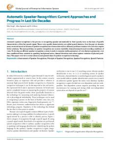
Figure 1: MAP adaptation of background keyword HMM to create target speaker keyword HMM.
µ ¯jm is the Gaussian mean of the adaptation data, µjm is the Gaussian mean of the background keyword HMM, and µ ˆjm is the updated Gaussian mean. Figure 1 illustrates MAP adaptation using MFCC features for a given keyword. A sequence of feature vectors (f1 , ..., fN ) belonging to instance i of keyword W in test conversation side t is scored against target speaker model MT S as follows:
Score(i, W, t, MT S ) = log
„
p(f1 , ..., fN |MT S ) p(f1 , ...fN |MBKG )
«
(3)
where MBKG is the background keyword HMM, and
For each target speaker, an HMM is trained for each keyword, using keyword-constrained MFCC features from eight conversation sides of target speaker data. Eight conversation sides are used to provide sufficient keyword HMM training data, because not all keywords may exist in a single conversation side. For each keyword, training is done via MAP adaptation from the background keyword HMMs. MAP adaptation provides a certain consistency between the background and target speaker HMMs, such that if a keyword does not exist among the target speaker conversation sides, the target speaker keyword HMM is the same as the background keyword HMM. Only the Gaussian mixture means are altered, via HTK, as follows: for state j and Gaussian mixture m [6][10]:
(4) where x is the sequence of all allowable states. An overall keyword score for a trial is obtained by adding the scores and dividing by the total number of frames for all instances of the keyword in test conversation side t. A keywordcombined score is obtained by applying this procedure across all instances of all keywords in the test conversation side.
Njm τ µ ¯jm + µjm (2) Njm + τ Njm + τ where τ is the weight of a priori knowledge to the adaptation data, Njm is the occupation likelihood of the adaptation data,
The supervector keyword HMM system, which we introduced in [7], is an extension of the keyword HMM system. Instead of computing the log-likelihoods and scoring each test conversation side as in the keyword HMM approach, the MAP adapted
µ ˆjm =
log(p(f1 , ..., fN |M )) = log(
X
p(f1 , ..., fN |x, M )p(x|M ))
x
4. Approach 1: The supervector keyword HMM system
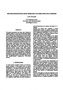
Figure 2: Obtaining supervector from MAP adapted Gaussian mixture means.
Gaussian mixture means of each target speaker keyword HMM are used as features in an SVM classifier. The 40-dimensional Gaussian mixture mean vectors of each component of each emitting state are concatenated to form a high-dimensional supervector. The supervector concept is introduced by Campbell et al. [8] in a system using GMMs instead of HMMs as statistical models. Figure 2 illustrates this process. 4.1. SVM training with supervectors As in [8], an SVM classifier with a linear kernel is trained for each target speaker, using the SV M light software package [11]. For each target speaker, the supervector obtained from its keyword HMM acts as the positive SVM training example, supervectors from keyword HMMs trained from 1,330 example impostor speakers [8] act as negative training examples, while those from keyword HMMs trained using data from single test conversation sides act as SVM test examples. The same MAP adaptation is used to train keyword HMMs for example impostor speakers (using eight conversation sides) and single test conversation sides. The SVM training approach as described above implies that each target speaker SVM is trained with only one positive training example (the supervector from the target speaker keyword HMM). To increase the number of positive training examples, different subsets of the eight conversation sides for a target speaker can be used (in a round-robin) to train a keyword HMM per subset, and supervectors from keyword HMMs from all subsets can be used as positive training examples. Hence, this round-robin training gives as many positive training examples as the number of subsets. Note that this is in contrast to the SVM training approach of [8], which uses one target speaker supervector per conversation side (the possible absence of keyword instances in single conversation sides prevents us from doing the same). Figure 3 illustrates the round-robin training
Figure 3: Target speaker round-robin training for SVMs.
process. Different weights can be assigned to SVM training errors for positive and negative training examples. Because there are still many more negative training examples than positive training examples for each target speaker even after subset selection, giving the positive example training errors more weight compared to negative example training errors seems desirable. Once an SVM is trained for each target speaker, they are used to classify supervectors from keyword HMMs trained from single test conversation sides. If a keyword is missing in a test conversation side, the supervector from the corresponding background keyword HMM is used as a substitute. The classification score for a test conversation side supervector against a target speaker SVM model is the score for that particular trial. The above approach trains one SVM for each target speaker from the corresponding keyword HMM, such that the speaker discriminative power of each keyword can be determined separately. To combine the keywords, supervectors obtained from all keyword HMMs for a target speaker can be concatenated into one higher-dimensional supervector for the target speaker (the same must be done for each example impostor speaker and test conversation side). SVM training and testing, as previously described, can be performed using the higher-dimensional supervectors to determine the combined speaker discriminative power of all keywords.
5. Approach 2: The phone lattice keyword HMM system This system is another extension of Boakye’s keyword HMM system, and uses the same training and testing paradigm. How-
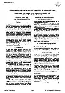
ities of the most probable paths extending from the beginning and end of that edge sequence. If there are multiple instances of the same phone sequence among the keyword-constrained edges, global probabilities for each instance are summed to obtain an overall global probability for the sequence. Keywordconstrained phone sequences are ranked according to their overall global probabilities, and the top N sequences are used for keyword HMM training. Note that this entire procedure of phone sequence extraction is only for a particular keyword instance and conversation side. The procedure must be repeated for all keywords instances and conversation sides. The following 48 phones, obtained from SRI, are used: aa, ae, ah, ao, aw, ax, ay, b, ch, d, dh, dx, eh, er, ey, f, fip, g, hh, ih, iy, jh, k, l, lau, m, n, ng, ow, oy, p, pau, puh, pum, r, s, sh, t, th, uh, uw, v, w, y, z, zh, < s >, < \s >. Note that some of the phones, such as pau, lau, < s >, < \s > are not actual phones, but symbols that represent various aspects of conversational speech. pau represents a pause, or silence, lau represents laughter, < s > represents the start of a phone sequence, and < \s > represents the end of a phone sequence. 5.2. Keyword HMM training
Figure 4: Extraction of top N keyword-constrained phone sequences
ever, instead of using MFCC feature sequences to train each keyword HMM, phone sequences are used. The nature of the keyword HMMs, such as the number of states, ergodicity, and output probability distributions, also differ. Because phone sequence data is far more sparse than the 40-dimensional MFCC feature sequences, this approach uses considerably less data and model parameters compared to the other approaches. 5.1. Extraction of phone sequences Each keyword HMM is trained using a set of keywordconstrained phone sequences, extracted from phone lattice decodings (where each edge represents a particular phone and its acoustic probability, and each node represents a particular time in the conversation side). For each keyword instance and a given conversation side, the top N most probable phone sequences formed by phone lattice edges falling within the time boundaries of the keyword (a keyword-constrained lattice segment) are considered. The global path probabilities of each keyword-constrained phone sequence must be computed. These probabilities are estimated by finding the most probable paths (via Dijkstra’s algorithm) from the first lattice node (in terms of time) to the nodes at the beginning of the keyword-constrained lattice segment, and from the last lattice node to the nodes at the end of the segment. Because the phones corresponding to edges outside of the keyword-constrained segment are not considered, these most probable paths have no phones associated with them. This entire procedure is shown in figure 4. The global probability of a particular keyword-constrained phone sequence is the product of the probabilities of each edge along its keyword-constrained edge sequence, and the probabil-
Once the phone sequences for a particular keyword are obtained, keyword HMMs are trained. Each of the 48 phones are assigned an integer value from 1 through 48, such that each phone sequence represents a sequence of discrete values. Hence, keyword HMM states have multinomial output probability distributions with 48 outputs. All HMMs have 2 emitting states. Because each phone sequence is typically only 6 to 7 phones in length (extremely short), HMMs with more than the minimum number of states would result in over-training, and decreased performance (experimentally determined). The HMMs are also ergodic, since in a given phone sequence, any phone can transition to any other phone, implying that restrictions should not be imposed over HMM state transitions. For a given keyword, the top N phone sequences (in terms of global probabilities) from each background conversation side are used to train the background keyword HMM (using the HTK software). As with the keyword HMM system, the background keyword HMM parameters are obtained using the Viterbi alignment and EM algorithms (but with multinomial output probabilities). If a keyword does not exist among the target speaker conversation sides, the target speaker keyword HMM is the same as the corresponding background keyword HMM. Target speaker keyword HMM training is done in a similar fashion as background keyword HMM training. One keyword HMM is trained for each target speaker via the EM algorithm, with parameters initialized with those from the corresponding background keyword HMM. Like the keyword HMM system, eight conversation sides of target speaker data are used to train each HMM. When a keyword appears more than once in a conversation side, the top N sequences from each keyword instance can be obtained, and the entire set of top N sequences can be used to train a keyword HMM. Note that this method implicitly gives higher HMM training weight to phone sequences that appear more than once among the keyword instances, since those sequences appear more than once in the HMM training data. For a given keyword W , top N phone sequences from each test conversation side t are scored against a target speaker model MT S . The score for phone sequence i is computed via the standard log-likelihood ratio (like the keyword HMM approach):
LLR(i, t, MT S , W ) = log(
p(ph1 , . . . , phT |MT S ) ) (5) p(ph1 , . . . , phT |MBKG )
where MBKG is the background keyword HMM, T is the length of the phone sequence. Note that keyword W , as used in the above equations, encapsulates all instances of the keyword, such that phone sequence i can be any phone sequence belonging to any instance of keyword W in test conversation side t. Similar to the keyword HMM approach, the score for a trial for keyword W is computed by averaging the likelihood ratios of all phone sequences constrained by the keyword in test conversation side t, and the keywords can be combined by averaging the likelihood ratios across all keywords in the test conversation side.
6. Approach 3: The keyword phone N-grams system This system, which we introduced in [9], examines the speaker discriminative power of keyword-constrained phone N-gram counts using an SVM classifier. Unlike the previous HMMbased system, time-dependent relationships among keywordconstrained phones are removed, and only their counts are used for training and testing. This approach is inspired by an approach that uses non keyword-constrained phone N-gram counts in a similar SVM classifier [4]. 6.1. Phone N-gram counts extraction For a given keyword, the phone N-gram counts extraction procedure is similar to the extraction of top N keyword-constrained phone sequences in the previous system, in that a phone lattice segment consisting of edges falling within the time boundaries of the keyword are obtained, and the global path probabilities from beginning and ends of the lattice to the segment are estimated via Dijkstra’s algorithm. However, instead of computing the global probabilities of entire phone sequences within the lattice segment, the probabilities of phone N-grams are desired. An estimate of the global probability P (Ni |W, C) for phone N-gram Ni constrained by keyword W in conversation side C is computed as follows:
P (Ni |W, C) =
P P j
k
p(Sk |Wj , C)count(Ni |Sk ) count(W |C)
(6)
where Sk is a phone sequence constrained by keyword W , count(Ni |Sk ) is the number of occurrences of phone N-gram Ni along phone sequence Sk , and count(W |C) is the number of instances of keyword W in conversation side C. The estimated probabilities of all phone N-grams (typically of orders 1, 2, and 3) for a particular keyword and conversation side is used as a feature vector in the SVM classifier (after a minor weighting of the features). 6.2. Keyword combination As with the previous approaches, results can be obtained for each keyword separately by using only the phone N-gram features constrained by each particular keyword. Different keywords can be combined at the feature level by concatenating the feature vectors for the different keywords within a conversation side (similar to the keyword-combination approach for the supervector keyword HMM system). Training, testing and scoring are completed on these larger feature vectors.
Because not all keywords appear in all conversation sides, phone N-gram data for a particular keyword in a conversation side may not exist, and are assigned feature values of 0. This is undesirable, since the values of 0 do not accurately reflect phone N-gram probabilities should the keyword exist in the conversation side. This missing data problem can be avoided by choosing high frequency keywords, with the majority of conversation sides containing most or all of the keywords. Note that a second way to address the missing data problem is by substituting the missing values with existing background values. This approach, however, has been experimentally determined to perform poorly. 6.3. SVM training, testing, and scoring As with the supervector keyword HMM approach and the approach for the non keyword-constrained phone N-grams system [4], an SVM with a linear kernel is trained for each target speaker (via the SV M light software package [11]). For each target speaker, the feature vectors belonging to 8 target speaker conversation sides are used as positive training examples, while the vectors belonging to all background conversation sides are used as negative training examples. To obtain a score for a trial, the test conversation side feature vector is scored against the target speaker SVM model.
7. The keywords A total of 62 keywords are involved in the four systems. Some are among the common discourse markers, back-channels, and filled pauses [6]. Certain keywords are chosen based on their perceived inter-speaker variability in pronunciation, while others are chosen based on frequency (to address the missing data problem in the keyword-constrained phone N-gram counts system). The keywords are the following – a, about, actually, all, and, anyway, are, be, because, but, do, for, get, have, i, if, i know, i mean, in, is, i see, it, i think, just, know, like, mean, my, no, not, now, of, oh, okay, on, one, or, people, really, right, see, so, that, the, there, they, think, this, to, uh, uhhuh, um, was, we, well, what, with, would, yeah, yep, you, you know, you see. Among these, the following 18 keywords – actually, anyway, i know, i mean, i see, i think, like, now, okay, right, see, uh, uhhuh, um, well, yeap, yep, you know, you see – are used in the keyword HMM system [6] (note that 19 keywords are used originally, but one keyword lead to degeneracy among the Gaussian mixture components of HMMs, and will not be used), and represent ∼15% of total background conversation side duration. Also, the following 52 unigrams among the 62 keywords – a, about, all, and, are, be, because, but, do, for, get, have, i, if, in, is, it, just, know, like, mean, my, no, not, of, oh, okay, on, one, or, people, really, right, so, that, the, there, they, think, this, to, uh, uhhuh, um, was, we, well, what, with, would, yeah, you – represent high-frequency unigrams, each occurring more than 4,000 times in the background conversation sides. Note that the 62 keywords represent ∼42% of background conversation side duration, with the 52 unigrams representing the majority (∼41%) of this duration. Since different keywords are typically better suited for different approaches, different subsets of the 62 keywords are examined for each system. A major goal is to examine the performance of keywords, especially as it relates to their lengths and frequencies, in different settings.
SRE06, using 16,831 trials with 2,010 true speaker trials. Also shown are results for two non keyword-based baseline systems – a cepstral GMM system [13] and a non keyword-constrained phone N-grams system [4], both with T-norm added [14]. Note that the non keyword-constrained phone N-grams system uses a larger background set (6,117 conversation sides), and that the two non keyword-based systems use more data by requiring entire speech conversation sides. System
Figure 5: Summary of similarities and differences among the approaches
8. Experiments and results The four approaches have various similarities and differences. In particular, the keyword HMM approach resembles the supervector keyword HMM approach, since both approaches use keyword-constrained acoustic features to train HMMs, and the phone lattice keyword HMM approach, since both approaches use the same log-likelihood based scoring in the keyword HMM framework. The phone lattice keyword HMM approach also resembles the keyword phone N-grams approach, since both approaches utilize only high-level keyword-constrained phone features. Lastly, the keyword phone N-grams and supervector keyword HMM approaches utilize the SVM classifier for testing and scoring. Figure 5 summarizes the similarities and differences among the approaches. Comparisons using various subsets of the 62 keywords are made for the similar approaches. 8.1. Keyword combination results The keyword-combination results examine the effectiveness of the collective power of a set of keywords for each system. The set of 18 keywords (19 minus you see) of the keyword HMM system, along with 20 of the 52 high-frequency unigrams – about, all, because, but, have, just, know, mean, no, not, one, people, really, so, that, there, think, this, was, what – are examined for the HMM-based systems (a total of 38 keywords are used). These 20 unigrams are selected based on their length, as each resulted in at least 5 HMM states for the acoustic keyword HMM systems. Note that these 38 keywords represent ∼26% of background conversation side duration. Because the keyword phone N-grams system requires keywords of high frequency due to the missing data problem, the 52 high-frequency unigrams are chosen. The 52 keywords are also used for the phone lattice keyword HMM approach. For the supervector keyword HMM system, a weight of 1 is given to weigh the positive versus negative SVM training errors, and round-robin training using subsets of 3 conversation sides is used to give 8 positive training examples per target speaker. For the keyword phone N-grams system, a weight of 500 is used, phone N-grams of order 1, 2, and 3 are extracted as features, and the top ∼33K features, in terms of frequency among the background conversation sides, are used. For the phone lattice keyword HMM system, the 40 most probable phone sequences (in terms of global probability for each keyword instance) are used for HMM training. Table 1 shows the keyword-combination results for the various systems (along with the speaker model complexity of each system), on the 8-conversation side task of
Keyword HMM Keyword HMM Appr. 1: SVHMM Appr. 1: SVHMM Appr. 2: PLHMM Appr. 2: PLHMM Appr. 2: PLHMM Appr. 3: KPN Non keywordconstrained phoneN-grams baseline GMM baseline
# of keywords
EER (%)
18 38 18 38 18 38 52 52
5.5 5.0 4.9 4.3 20.7 16.9 13.7 5.0
# of speaker model parameters ∼50K ∼110K ∼250K ∼440K ∼1.8K ∼3.8K ∼5.2K ∼260K
– –
5.2 4.6
– –
Table 1: Keyword combined results. Using 38 keywords (∼26% of speech data), the supervector keyword HMM system (4.3% EER) out-performs all other systems. It shows a 6.5% relative improvement over the GMM baseline (4.6% EER), and a 17.3% improvement over the non keyword-constrained phone N-grams baseline (5.2% EER). The supervector keyword HMM system (4.3% EER) achieves a 14.0% improvement over the keyword HMM system (5.0% EER), and a 74.6% improvement over the phone lattice keyword HMM system (16.9% EER). Using the 52 high-frequency keywords, the keyword phone N-grams system (5.0% EER) achieves a 3.8% improvement over the non keyword-constrained phone N-grams baseline (5.2% EER). This result directly demonstrates the effectiveness of focusing modeling power on the informative regions of conversation sides containing the keywords, since the keyword phone N-grams system uses the methodology of the non keyword-constrained system, but applied to each keyword separately. The keyword phone N-grams system also achieves a 63.5% improvement over the phone lattice keyword HMM system (13.7% EER). However, the system uses ∼41% of background conversation side data compared to the ∼26% used for the keyword HMM and supervector keyword HMM systems. Recall that both the keyword phone N-grams and supervector keyword HMM systems are SVM-based, with feature vectors having ∼33K and ∼55K dimensions respectively. Hence, with the exception of the keyword HMM system using 38 keywords, which has the same EER (5.0%) as the keyword phone N-grams system, SVM-based approaches relying on high-dimensional feature vectors outperform the other approaches. Note that the phone lattice keyword HMM system uses significantly fewer model parameters than other keyword-based systems. Also, unlike the acoustic feature-based systems, the phone lattice keyword HMM system uses a very sparse form of speech data (phone sequences versus 40-dimensional MFCC feature sequences) to train its keyword HMMs. Hence, it is not
surprising to observe a drop-off in performance for this system. The results also demonstrate the benefits of using more keywords. Increasing the number of keywords from 18 to 38 results in an 12.2% improvement for the supervector keyword HMM system (4.9% EER to 4.3% EER), and a 9.1% improvement for the keyword HMM system (5.5% EER to 5.0% EER). However, as more keywords are used, one advantage of using keyword-constraining, namely, reducing the amounts of speech data required, diminishes. The 38 keywords (∼26% of background data) represent a ∼60% increase in data over the 18 keywords (∼15% of background data). This increase in data usage greatly increases the need for memory and computation when implementing the systems. 8.2. Individual keyword results The individual keywords are examined to see how each would perform in the various approaches, under the optimal set of parameters as previously described. Because not all keywords exist in all conversation sides, individual keyword results only involve trials where the keyword exists in both the target speaker and test conversation sides. Individual results for the 38 keywords are obtained for the supervector keyword HMM and keyword HMM systems. Table 2 shows results for the top 15 keywords (in terms of performance) of the keyword HMM system, which has the best individual results on the SRE06 8 conversation side task. Also shown are the individual keyword results for the supervector keyword HMM system, the number of occurrences of the keyword in background conversation sides, and the number of keyword HMM states for the MFCC featurebased HMM systems. Note that these keywords are also experimented with for the phone lattice keyword HMM system. However, results are significantly worse. Individual results for the 52 high-frequency unigrams are also obtained for the phone lattice keyword HMM (PLHMM) and keyword phone N-grams (PLN) systems, and the top 20, according to the keyword phone N-grams system, are shown in table 3. Note that for the 38 keywords, if a keyword unigram is part of a keyword bigram, those unigram instances are ignored. For the 52 unigrams, no keyword instances are discarded. EER (%) results Keyword yeah you know i think right um that because like i mean but people so have just not
HMM 11.4 11.9 14.7 14.7 14.8 14.9 15.2 15.2 15.8 16.6 17.2 17.4 18.0 18.1 18.3
SVHMM 17.0 17.5 23.5 22.7 19.3 19.2 24.1 21.7 26.8 22.9 26.5 24.7 25.4 28.4 26.0
Other statistics # of HMM instances states 26,530 6 17,349 8 6,288 9 8,021 8 11,962 6 26,277 5 5,164 8 18,058 5 5,470 8 12,766 5 4,906 8 14,291 6 9,610 5 8,660 6 6,817 5
Table 2: Individual keyword results for keyword HMM and supervector keyword HMM systems
EER (%) results Keyword know i and yeah like you that think right because but people really um to mean the so have they
PLA 24.1 24.7 24.8 26.1 26.1 26.9 27.3 28.3 29.0 29.1 29.8 30.5 30.7 32.2 32.2 32.4 32.7 33.3 33.4 34.7
PLHMM 26.1 25.2 28.7 29.7 26.7 28.9 30.1 32.9 30.2 32.3 32.6 34.6 32.2 30.7 33.2 35.0 34.6 34.5 35.2 35.9
# of instances 24,258 59,622 37,878 26,530 18,058 39,093 26,277 9,467 8,021 5,164 12,766 4,906 6,674 11,962 27,224 5,724 31,606 14,291 9,610 12,436
Table 3: Individual keyword results for phone lattice keyword HMM and keyword phone N-grams systems
According to both tables, keywords that perform relatively well for one system tend to perform well for the others. Results show that individual keywords generally perform better in the acoustic features framework, with significant improvements from the phone lattice keyword HMM and keyword phone Ngrams systems, to the keyword and supervector HMM systems. This is demonstrated by the keyword yeah (among many others), which shows a 56.3% improvement in EER (26.1% to 11.4%) from the keyword phone N-grams to keyword HMM systems. In addition, there is improvement in individual keyword EER from the supervector to the keyword HMM system (a 32.9% improvement for yeah, from 17.0% to 11.4%), in contrast to the 14.0% improvement from the latter to the former in the keyword-combination experiments. The keyword phone N-grams system shows a modest improvement from the phone lattice keyword HMM system (a 12.1% improvement for yeah, from 29.7% to 26.1%). This is in contrast to the 63.5% improvement achieved in the keywordcombination experiments. This suggests that SVMs (used by the keyword phone N-grams system) perform exceedingly well in feature-level combination, such that increasing the dimensionality of the overall feature vector (via concatenation of features) leads to significantly improved results. Whereas the feature vectors in the keyword-combination experiments are over 30K in dimension, they are typically of 1,000 to 2,000 in dimension in the individual keyword experiments. Overall, these results suggest that while systems relying on phone features can match or exceed performances of acoustic feature-based systems in keyword-combination experiments, the sparseness of the high-level phone features compared to the acoustic features leads to significantly worse results when keywords are examined separately. Keywords that perform well (i.e. yeah, you know) generally occur more often in the background conversation sides. This is especially true for the supervector keyword HMM system,
where 6 of the top 7 performing keywords (yeah, you know, that, um, like, but) rank among the top 10 in occurrences. While keyword performance is positively correlated with keyword frequency, keyword length (approximately represented by the number of keyword HMM states), appears to be less of a factor. However, some keywords of high length (i mean, people) have low frequency, while 4 of the top 7 keywords for the keyword HMM system have eight or more HMM states. Hence, given more data such that more instances of keywords with high numbers of HMM states can be used for training and testing, it may be possible to discover a clear positive correlation between keyword performance and length.
9. Conclusion We have discussed and compared four speaker recognition systems relying on word-conditioning: the keyword HMM, supervector keyword HMM, phone lattice keyword HMM, and keyword phone N-grams systems. We also examined the performances of 62 keywords (representing ∼42% of background conversation side duration) of various lengths and frequencies in both keyword-combination experiments and individual keyword experiments using the above approaches. We have shown that the SVM is an effective classifier for keyword-combination experiments with very high dimensional feature vectors. The effectiveness of the SVM in this framework appears to compensate for features that perform poorly in the individual keyword setting (i.e. phone N-grams). Acoustic features perform significantly better in the individual keyword setting, and achieve the best result in conjunction with the SVM in keyword-combination. The effectiveness of acoustic features with SVMs in keyword combination is demonstrated by the supervector keyword HMM system, which achieves a 0.3% absolute EER improvement (4.6% to 4.3% EER) over the GMM baseline (our best baseline) on the SRE06 8 conversation side task. The keywords yeah and you know have the best individual keyword results. An extension we are currently working on is to augment the supervectors of the supervector keyword HMM system using long-term, prosodic features, in an attempt to increase the speaker-discriminative power of the keywords.
10. References [1]
Reynolds, D., “Speaker Identification and Verification using Gaussian Mixture Speaker Models”, in Speech Communication, Vol. 171-2, pp. 91–108, 1995.
[2]
Doddington, G., “Speaker Recognition based on Idiolectal Differences between Speakers”, in Proc. of Eurospeech, pp. 2521–2524, 2001.
[3]
Andrews, W., Kohler, M., Campbell, J., “Phonetic Speaker Recognition”, in Proc. of Eurospeech, pp. 149– 153, 2001.
[4]
Hatch, A., Peskin, B., Stolcke, A., “Improved Phonetic Speaker Recognition Using Lattice Decoding”, in Proc. of ICASSP, Vol. 1, pp. 169–172, 2005.
[5]
Sturim, D., Reynolds, D., Dunn, R., Quatieri, T., “Speaker Verification using Text-Constrained Gaussian Mixture Models”, in Proc. of ICASSP, Vol. 1, pp. 677–680, 2002.
[6]
Boakye, K., “Speaker Recognition in the TextIndependent Domain using Keyword Hidden Markov Models”, master’s report, UC Berkeley, 2005.
[7]
Lei, H., Mirghafori, N., “Word-Conditioned HMM Supervectors for Speaker Recognition”, to appear in Interspeech, 2007.
[8]
Campbell, W., Sturim, D., Reynolds, D., Solomonoff, A., “SVM Based Speaker Verification using a GMM Supervector Kernel and NAP Variability Compensation”, in Proc. of ICASSP, Vol. 1, pp. I-97–100, 2006.
[9]
Lei, H., Mirghafori, N., “Word-Conditioned Phone Ngrams for Speaker Recognition”, in Proc. of ICASSP, 2007.
[10] HMM Toolkit (HTK): http://htk.eng.cam.ac.uk [11] Joachims, T., “Making Large Scale SVM Learning Practical”, in Advances in kernel methods - support vector learning, B. Schoelkopf, C. Burges, and A. Smola, Eds. MIT-press, 1999. [12] Stolcke, A., Bratth, H., Butzberger, J., Franco, H., Rao Gadde, V., Plauche, M., Richey, C., Shriberg, E., Sonmez, K., Weng, F., Zheng, J., ”The SRI March 2000 Hub5 Conversational Speech Transcription System”, in Proc. NIST Speech Transcription Workshop, 2000. [13] Kajarekar, S., Ferrer, L., Venkataraman, A., Sonmez, K., Shriberg, E., Stolcke, A., Gadde, R.R., “Speaker Recognition using Prosodic and Lexical Features”, in Proc. of the IEEE Automatic Speech Recognition and Understanding Workshop, pp. 19–24, 2003. [14] Bimbot, F., Bonastre J.F., Fredouille C., Gravier G., Magrin-Chagnolleau I., Meignier S., Merlin T., OrtegaGarca J., Petrovska-Delacrtaz D., Reynolds D.A., “A Tutorial on Text-independent Speaker Verification, in EURASIP Journal on Applied Signal Processing, Vol. 4, pp. 430–451, 2004.