appear to have nonâinteger values according to numerical estimates, notwithstanding the fact that the dimension of the full orbit (involving all times) is proved ...
Compatibility between dynamics and Tsallis statistics A. Carati Università di Milano, Dipartimento di Matematica Via Saldini 50, 20133 Milano (Italy). Abstract. We perform numerical simulations for the dynamics of a chain of weakly coupled particles, and consider the process of occupation of cells in phase space, in the spirit of paper [1]. A different behaviour is exhibited as the coupling constant is changed. It is discussed whether such a dynamical behaviour is compatible with the Tsallis statistics. Keywords: Time–averages, non–equilibrium thermodynamics, Tsallis distribution. PACS: 05.20.Gg, 05.45.-a, 05.70.Ln.
INTRODUCTION In the paper [1] (see also [2]), a method was introduced to deal with Statistical Thermodynamics if reference is made to dynamics through time-averages. This can be useful for example when one has to deal with metastable states, in which the system remains frozen far from equilibrium for very long times, so that it is not clear what measure in the phase space should be used. In agreement with the opinion expressed by most classics, one can make the statement that the macroscopic quantities observed are nothing but the time–averages (up to the observation time–scale) of the relevant dynamical variables. Indeed, if the system is ergodic, the time–averages over infinite times coincide with the Gibbs phase-averages, but there remains open the problem that nothing is known concerning the time–averages for large but finite times. For example, in the literature cases are reported (see [3]) in which the dimensions of the orbits of Hamiltonian system appear to have non–integer values according to numerical estimates, notwithstanding the fact that the dimension of the full orbit (involving all times) is proved (see [4]) to actually be an integer. This fact was explained in the paper [5]. There it was shown, for the familiar standard map, that the observed dimension actually depends on the observation time, and that the attainment of the “true value” (two in that case) would require an exceedingly large number of iterations (outside of the computers reach). This, notwithstanding the fact that, the fractal dimension appears to settle down to a definite non–integer value on a finite time–scale. It is clear that on time–scales of the latter type the sojourn time measure too has to appear very odd, i.e. non absolutely continuous with respect to the Lebesgue one. So, in general, if one has to deal with a metastable state (i.e. an “ergodic behaviour” is granted only on a times–scale much larger than the available one), then the orbits could exhibit some strange features (such as a non integer fractal dimension on the observed time–scale) which may prevent the use of the Gibbs measure. It has been suggested that in some problems where metastable states show up (as in systems of rotators with long–range coupling [6], or in galaxies [7]), one has to
replace the Gibbs measure by the Tsallis one [8]. On the other hand, in the paper [1] it was shown that the use of time–averages amounts to introducing a measure in phase space, suitably defined by the dynamics of the system. In short (see Section 2 for precise definitions) one has to determine the statistics of the sojourn times, and then the coarse–grained density of the phase–space measure turns out to be nothing but the (logarithm of the) Laplace transform of the p.d.f. of the sojourn time of any cell. In particular, the usual Gibbs measure is recovered if the dynamics is very chaotic, i.e. the p.d.f. (of the sojourn time) is a Poisson one. In this paper we numerically estimate the p.d.f. of the sojourn time for two models: a chain of next neighbours weakly coupled rotators, and a FPU β -model (i.e. a chain of next neighbours weakly coupled particles). Both models are know to exhibit a non ergodic behaviour: for high enough energy the first model (see for example [9]), for low enough energy the second (see the original paper of Fermi, Pasta and Ulam [10], or [11] for a review). The numerical results indicate that the the p.d.f. of the sojourn time is not a Poisson one; moreover using a Tsallis distribution (to be defined in Section 2) with the appropriate values for the parameters, one can fit the numerical data very well. The paper is organised as follows. In Section 2 the method to deal with time-averages is recalled. In Section 3 the models are described and the numerical results exhibited in Section 4.
TIME–AVERAGES We recall here, briefly, the method which was introduced in [1] in order to obtain the relevant thermodynamic functions on the basis of dynamics, namely when use is made of time–averages rather than of ensemble averages. Consider a diffeomorphism Φ on a phase–space M , and an orbit xn = Φ(xn−1 ), n = 1, . . . , N up to “time” N, determined by an initial value x0 . In our case, we deal with the orbits generated by iterations of the time–τ map induced by the flow of an Hamiltonian system. The time–average (up to time N) of a dynamical variable A(x) (a real function on M ) is defined by N
1 ¯ 0 )def A(x = ∑ A(xn ) . N n=1 Such a time–average can also be computed by partitioning the space M into a large number K of disjoint cells Z j (such that M = ∪Z j ), and reckoning the number of times n j (x0 ) the orbit {xn } visits any cell Z j (so that n j /N is the discrete analogue of the sojourn time, see also [12]). Indeed one has ¯ 0) ≃ A(x
K
nj
∑ Aj N
,
(1)
j=1
where A j is the value of A at a chosen point x ∈ Z j . In equilibrium statistical mechanics one considers the limit N → +∞, but in presence of metastable phenomena one has to consider time averages on some large but still finite time–scale. In the latter case it is
0.4
1
Poisson distribution, p=9/8
0.35 0.1 0.3 0.01 Poisson distribution, p=9/8 p.d.f.
p.d.f.
0.25
0.2
0.001
0.15 1e-04 0.1 1e-05 0.05
0
1e-06 0
2
4 6 Number of visits
8
10
0
2
4 6 Number of visits
8
10
FIGURE 1. Histogram of the occupation numbers for the rotators chain at temperature T = 0.25. The total integration time is 219 ≃ 5 105 . Left panel: normal scale; right panel: semi–logarithmic scale.
meaningful to think of N as a parameter having a fixed “large” value. In this case there is ¯ 0 ) is not almost constant nothing analogous to the ergodic theorem, i.e. the function A(x but does depend on the initial datum x0 . ¯ 0 ) turns If a certain probability distribution is assigned for the initial data x0 , then A(x out to be a random variable, in the sense that it will assume different values with different probabilities. It is then natural to consider the expectation value < A¯ > of the time ¯ 0 ) with respect to the initial data distribution, i.e. the quantity average A(x 1 < A¯ >= N
K
∑ Aj < nj > ,
(2)
j=1
where we have denoted by < · > the expectation with respect to the a priori distribution. This formula shows that the time average of every dynamical variable can be expressed in terms of the averages of the random variables n j (x0 ), so that the probability distribution function Fj (n) of the occupation number n j turns out to have a fundamental role. Our aim is to give a numerical estimate of the function F(n j ), and to check if it is compatible with a thermodynamics given by a Tsallis statistic. Notice that, in statistical thermodynamics one does not deal directly with the a priori probability, because it is generally assumed that the time–average of the energy of the system has a given value U , which should play the role of an independent variable. So we consider the energy of the system, which we denote by ε , and the corresponding time– average ε¯ = ∑ j ε j n j /N. One has then to impose on the numbers n1 , · · ·, nK the further condition N1 ∑Kj=1 ε j n j = U = const. Thus the quantity of interest is the a posteriori expectation of A¯ given U , which can by expressed in term of the a posteriori expectation
0.2
1
0.18
Poisson distribution, p=4.5
Poisson distribution, p=4.5 0.1
0.16 Tsallis distribution, σ=13, p=1 0.14 0.01
p.d.f.
p.d.f.
0.12 0.1
0.001
0.08 1e-04 0.06 0.04 1e-05
Tsallis distribution, σ=13, p=1. 0.02 0
1e-06 0
5
10 Number of visits
15
20
0
5
10 Number of visits
15
20
FIGURE 2. Histogram of the occupation numbers for the rotators chain at the same temperature T = 0.25 of Figure 1, but at larger total integration time (the total time is 221 ≃ 106 ). Left panel: normal scale; right panel: semi–logarithmic scale.
ν j =< n j >U of the occupation numbers by < A¯ >U =
1 A jν j . N∑ j
The quantities ν j /N are then the coarse–grained analogues of the density of the standard equilibrium measures. In particular standard Gibbs thermodynamics are recovered if ν j ≃ exp(−θ ε j ), while Tsallis statistics is obtained if ν j ≃ (1 − θ ε j )q . For large system one finds that ν j can be computed by making reference to a function χ j (z), which is the logarithm of the Laplace transform of the cumulative p.d.f. Fj (n). Namely defining χ j (z) by def
exp(χ j (z)) = one finds
Z
R
e−nz dFj .
(3)
� �ε θ j +α , (4) N where α and θ are determined imposing that the mean energy is U and the total number of iterations is N. In particular (see [1]), if the process of occupation of any cell is a Poisson one, i.e. if the successive visits of a given cell are independent events, one finds that ν j ≃ exp(−θ ε j ). Instead, the Tsallis q–distribution is obtained if the variables n j are distributed in such a way that � z �−σ def χ j (z) = χ T s (z) = p 1 + −p; (5) σ
ν j = −χ ′j
0.3
1 Poisson distribution, p=1
0.25
Poisson distribution, p=1
0.1 Tsallis distribution, σ=1.875, p=1 0.01
p.d.f.
p.d.f.
0.2
0.15
0.1
0.001
1e-04
0.05
1e-05 Tsallis distribution, σ=1.875, p=1
0
1e-06 0
5
10 Number of visits
15
20
0
5
10 Number of visits
15
20
FIGURE 3. Histogram of the occupation numbers for the rotators chain at temperature T = 0.5. The total integration time is 219 ≃ 5 105 . Left panel: normal scale; right panel: semi–logarithmic scale.
here p and σ are positive parameters, moreover σ is related to the so–called “entropic index” q by the relation σ = 1/(q − 1). From the Laplace transform χ T s (z) one can find the distribution F T s (n) of the occupation numbers, and then make a comparison with the actual finding in the numerical experiments. It turns out that F T s (n) doesn’t have a closed expression in terms of known functions, except for some special cases, but expression for F T s (n) can however be given as a series expansion (details can be find in ref. [13], see also [14]). In the next section we show that, by choosing appropriate values for p and σ , the function F T s (n) fits the distribution Fj (n) one gets from the numerical computations, in a better way with respect to a Poisson one.
THE MODELS So the problem becomes to estimate the function Fj (n) by numerical computation. Make this using the definition of Fj (n) requires a great computational power because one has to integrate a large number of orbits for long times. So we take a different approach. Consider the time flow map Φτ with τ sufficiently large, and compute just a single orbit, with an initial datum taken at random. Then, one takes a record of the cells the orbit visits and builds the histogram of how many cells are visited one time, how many cells are visited two time, and so on. In the hypothesis that the n j are independent and equidistributed (all Fj are equal to the same function F) this histogram is closed to Fj (n) (because for the law of the large numbers the frequency is closed to the probability). We have built such an histogram for two kind of system. A system of k = 16 rotators with Hamiltonian H = ∑ p2i /2 + 1/4 ∑ cos(φi+1 − φi ) ,
0.5
1 Poisson distribution, p=1.
0.45 Poisson distribution, p=1.
0.1
0.4
Number of visited cells
Number of visited cells
0.35 0.3 0.25 0.2
0.01 Tsallis distribution, σ=4., p=2. 0.001
1e-04
0.15 0.1 1e-05 Tsallis distribution, σ=4., p=2.
0.05 0
1e-06 0
2
4
6
8
10
0
2
4
Time
6
8
10
Time
FIGURE 4. Histogram of the occupation numbers for the FPU model at temperature T = .11. The total integration time is ≃ 5 108 . Left panel: normal scale; right panel: semi–logarithmic scale.
and periodic boundary conditions. We take initial data uniformly distributed for the angles φi , while the momenta pi are extracted from a Maxwell–Gibbs distribution with temperature T . We divided the phase space in 216 cells of equal (Gibbs) measure, in the following way: for each i = 1, . . ., k we consider the sets Ai = {|pi | < α T } ,
ACi = {|pi | > α T }
α = 0.6745 . . . being the quartile of the normal distribution. The cells are simply obtained by all the possible intersection ∩Bi , where Bi is either Ai or its complement ACi . We also consider a FPU system of k = 16 moving particles, i.e. a linear chain of particles coupled through non linear springs, with Hamiltonian H = ∑ p2i /2 + ∑(xi+1 − xi )2 + 1/4 ∑(xi+1 − xi )4 , and fixed end conditions. We take initial data distributed according to exp(−H2 /T ), H2 being the quadratic part of the Hamiltonian. The partition of the phase space is obtained considering 216 cells defined in the following way: denoting with Ei is the energy of the i-th normal mode, for each i = 1, . . ., k we considers the sets Ai = {Ei < log 2 T } ,
ACi = {Ei > log 2 T }
Notice that the value log 2 is the median of the normal mode energy distribution according to the Gibbs distribution (in the harmonic approximation). The cells are obtained as before by the all the possible intersection ∩Bi , being Bi either Ai or ACi .
0.5
1 Poisson distribution, p=1.
0.45 Poisson distribution, p=1.
0.1
0.4
Tsallis distribution, σ=1.4, p=2.25
0.35 0.01
p.d.f.
p.d.f.
0.3 0.25
0.001
0.2 1e-04 0.15 0.1 1e-05 Tsallis distribution, σ=1.4, p=2.25
0.05 0
1e-06 0
5
10 Number of visits
15
20
0
5
10 Number of visits
15
20
FIGURE 5. Histogram of the occupation numbers for the FPU model at temperature T = .06. The total integration time is ≃ 5 108 . Left panel: normal scale; right panel: semi–logarithmic scale.
NUMERICAL RESULTS The first three figures refer to the system of rotators. We recall that this system is integrable (i.e. not chaotic) in the limit of high energy, while it is expected to becomes very chaotic in the limit of low one. In Figure 1 is illustrated the histogram of the occupation number, for a temperature T = 0.25. As one can see, the fit with a Poisson distribution is quite good. But if we increase the integration time of a factor 4, the histogram departs from the Poisson distribution, as one can check from the data reported in Figure 2. Instead, the data can be represented in a very good way using a distribution F T s (n) with parameter p = 1 and σ = 13. If we rise the temperature the departure from a Poisson distribution happens at earlier times. This is illustrated in Figure 3, where the histogram of the occupation numbers, for a temperature T = 0.5, is reported. The integration time is the same as that of Figure 1. We see that the departure of a Poisson distribution is clear, and also that a distribution F T s (n) with parameter p = 1 and σ ≃ 1.9 agrees very well with the numerical data. One can ask for the dependence of the parameter p and σ both on time and on the size of the system. For example, the dependence of σ from the particles number k is crucial, because if σ → ∞ for k → ∞ then, in the thermodynamical limit, one would obtain again the Gibbs distribution. We have not deal with this fundamental question, because this is only a preliminarily work, aimed at showing that Tsallis distribution is compatible with the dynamics of simple Hamiltonian systems. The histograms for the FPU model show the same behaviour. In Figure 4, the data for the FPU model at temperature T = .11 are reported. Looking at the data in the left panel, one can see that the Poisson distribution gives a good fit. But, looking at the data in semi–logarithmic scale (right panel), one can check that the Poisson distribution fails in the tail of the distribution, whereas a distribution F T s (n) with parameters p = 2 and
σ = 4 seems to agree better with the data, in the whole range. It is true that the tail of the distribution is computed with a lower precision than the bulk (where the Poisson distribution and the Tsallis one agrees), so that this test could also be considered not very significant. But data computed at the lower temperature T = .06, indicate that a Poisson distribution is not adequate also in the bulk of the histogram, as one can clearly see from Figure 5. On the contrary a Tsallis distribution F T s (n), with p = 2.25 and σ = 1.4, seems to fit the data in a quite good way. In conclusion, this preliminary numerical results seem to indicate that the distribution of the sojourn time in not a Poisson one for system which are only weakly chaotic. If this is the case, the Maxwell–Gibbs measure is not the appropriate one to use in statistical thermodynamics computations. At the same time, the numerical results also show that the distribution of the sojourn time is compatible with the Tsallis one. Obviously, more numerical confirmations are need, besides a study of the dependence’s of the quantities p and σ from the parameters entering the system.
REFERENCES 1. 2. 3. 4. 5. 6. 7. 8. 9. 10. 11. 12. 13. 14.
A. Carati, Physica A 348, 110–120 (2005). A. Carati, Physica A 369, 417–431 (2006). M. Pettini, A. Vulpiani, Phys. Lett. A 106, 207 (1984). S.E. Newhouse, Soc. Math. France, Astérisque 51, 223 (1978). G. Benettin, D. Casati, L. Galgani, A. Giorgilli, L. Sironi, Phys. Lett. A 118, 325 (1986). V. Latora, A. Rapisarda, C. Tsallis, Physica A 305 129 (2002); V. Latora, A. Rapisarda, C. Tsallis, Phys. Rev. E 64 056134 (2001). A.R. Plastino, A. Plastino Phys. Lett. A 174, 384 (1993); J.J. Aly, J. Perez, Phys. Rev. E 60, 5185 (1999); T. Kronberger, M.P. Leubner, E. van Kampen, Astronomy&Astrophysics 453, 21–25(2006). C. Tsallis, J. Stat. Phys. 52, 479 (1988). R. Livi, M. Pettini, S. Ruffo, A. Vulpiani, Jour. Stat. Phys. 48, 539 (1987). E. Fermi, J. Pasta and S. Ulam, “Studies of nonlinear problems” in E. Fermi: Note e Memorie (Collected Papers) Vol. II, edited by E. Segrè et al., Accademia Nazionale dei Lincei, Roma, and The University of Chicago Press, Chicago, 1965, pp. 977–988. A. Carati, L. Galgani, A. Giorgilli, Chaos 15, 015107 (2005). C. Beck, F. Schloegl, Thermodynamics of Chaotic Systems, Cambridge University Press, Cambridge, 1993, pp. 20–21. A. Carati, On the fractal dimension of orbits compatible with Tsallis statistics, to appear in Physica A. S. Abe, Y. Nakada, Physical Review E 74, 021120 (2006).