Compatibility Determination in Web Services Yunyao Li
H.V. Jagadish
Department of EECS University of Michigan
Department of EECS University of Michigan
Ann Arbor, MI 48109, USA +1 734 763-5243
Ann Arbor, MI 48109, USA +1 734 763-4079
[email protected]
[email protected]
ABSTRACT Determining the compatibility between Web services plays a critical role in supporting dynamic discovery and collaboration of Web services in the inherently heterogeneous web environment. In this paper we present a compatibility determination algorithm. The algorithm takes two graphs (each representing the external interface of a Web service) as inputs, and produces the following as outputs (1) judgment of compatibility (true or false), and (2) differences between two graphs. The outputs can be used by a Web service to enable dynamic collaboration between Web services. A visualized representation of differences found can enable a human to determine the criticality of the differences.
Categories and Subject Descriptors H.2.1 [Information Systems]: Database Management - Logical Design; H.5.3 [Information Systems]: Group and Organization Interfaces - Web-based interaction, Asynchronous interaction
General Terms Algorithms, Verification, Design
Keywords Web services, compatibility, matching, business process
difference
detection,
graph
1. INTRODUCTION Web services are generally described as self-contained, selfdescribing, modular applications that can be published, located, and invoked across the web [1]. Ultimately, web services should be able to dynamically discover other Web services and interact with them automatically without human involvement, just like the open, ubiquitous connectivity the Web has enabled for person-toperson communications. To support collaboration processes between business partners, electronic commerce standards such as Electronic Business XML (ebXML) [2], the Web Service Conversation Language (WSCL) [3] and Business Process Execution Language for Web Services (BPEL4WS) [4] have been developed. Permission to make digital or hard copies of all or part of this work for personal or classroom use is granted without fee provided that copies are not made or distributed for profit or commercial advantage and that copies bear this notice and the full citation on the first page. To copy otherwise, or republish, to post on servers or to redistribute to lists, requires prior specific permission and/or a fee. ICEC03, Month 9-10, 2003, Pittsburgh, PA Copyright 2000 ACM 1-58113-000-0/00/0000…$5.00.
All these standards requires a Web Service to publish its external interface, describing operations requesting services from service providers or offering services to service requestors. Such an external interface of a Web service defines how a Web service could interact with other Web services [5], and is referred as the business process interaction (BPI) model in this paper. To ensure correct interactions between Web services in a dynamic collaboration, ebXML requires that all the participating Web services share the same BPI model, while other standards currently do not even support dynamic discovery and collaboration of Web services [6]. None of these standards directly address the significant problem of how to handle the discrepancies between the BPI models of Web services. The existences of discrepancies between the BPI models of two Web services may not necessarily prevent them from interoperate with each other [7]. For example, let Service A and Service B be services from different companies. Suppose that the buyer Service A wants to engage in a seller-buyer interaction with the seller Service B. Service A and Service B may not share the same BPI model for the sell-buyer interaction. For instance, Service A does not require the ability of canceling order, while Service B provides this facility. Similarly, Service A requires the ability to change the order, while Service B does not provide such a facility. Some of the differences, such as latter difference in the above example may affect their interoperability; other differences, such as the former one, may be immaterial to the collaboration, since Service A could always choose not to cancel an order even if service B allows it. Moreover, the external interface published by a Web service may not necessarily be the only interaction process it supports. In the above buyer-seller example, a Web service A’s internal business rules may require the ability of canceling order when the total amount of order is over $10,000, while not requiring it for other orders. Such dynamic configurable internal business process may not be able to be represented by one BPI model, while it is not feasible to require a Web service to reveal all of the interaction processes it supports. It is important for a Web service to be able to automatically detect the differences between its BPI model from that of others’. Such information is critical for the Web service to whether and how to change its own business process to enable the collaboration with Web services, for negotiation between Web services. It also provides useful reference for future Business Process Reengineering. In this paper, we propose an efficient algorithm to support automatic compatibility determination of BPI models between Web services. Specifically, we take the BPI models defined in ebXML as the basis for developing our algorithm. EbXML is a widely recognized electronic commerce standard supporting
dynamic collaboration of Web services [6]. The BPI model defined by ebXML is generally compatible with other standards involving Web Service. It is reasonable to expect that future standards developed with the intent to support dynamic collaboration of Web services will have similar characteristics as ebXML. Thus our ideas discussed in this paper should be still applicable to such electronic business standards.
2. OVERVIEW AND PRELIMINARIES In Section 2.1, we introduce BPI model in ebXML. Details of the graph representation of a BPI model used in our paper follow in Section 2.2. In Section 2.3, we give a brief overview the BPI model Difference Detection problem using an example.
2.1 Introduction to ebXML BPI model We can represent the external interface of a Web service as BPI model. In ebXML, we can consider a Business Collaboration represented by Business Process Schema as a BPI model. (Hereafter, when we use the term “Business Collaboration” or “Business Process” we mean BPI model.) ebXML Business Process Schema provides the semantics, elements and properties necessary to define Business Collaborations [2]. Two or more business partners participate in a Business Collaboration through roles. The roles interact with each other through Business Transactions. The business transactions are sequenced relative to each other in a “Choreography”. Each Business Transaction consists of one or two predefined Business document flows. The basic semantics of Business Collaboration are as shown in figure 1.
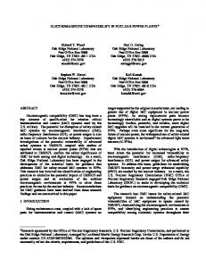
conditionGuard label marking the condition under which the transition occurs. Adjacency matrix representation is used to represent the directed graph described above. Each element of the matrix A (aij) is defined as the following: 1, if (i, j ) ∈ E ,&conditionGuard = Success 2, if (i, j ) ∈ E ,&conditionGuard = NoGuard aij = − 1, if (i, j ) ∈ E ,&conditionGuard = Failure 0, otherwise
Figure2 shows the graph representation of a BPI model. The number inside each node is the node’s identifier. The label beside each node represents the Business Transaction or the type of Join that the node associated with. Such labels are for readability only, and are not used in the algorithm. The number beside each edge is the value of corresponding element in the adjacency matrix.
1 Failure
OrderTBA
Success Fork
3 Failure
4
2
CancelOrderTBA
ChangeOrderTBA
OrderStatusTBA Success
Success Failure
Failure
No Guard
5
Failure
Success
1 1 -1
2 Change
1 -1
-1
Order 1
3
4 Cancel
-1
2
CheckOrderStatus
5
Figure 1. Basic semantics of Business Collaboration In this paper, we consider BPI models involving two Web services. However, this analysis can be easily extended to situations involving multiple Web services.
Join
Figure 2. Example of BPI model Graph Representation
2.3 Overview of The Problem
V: Set of nodes in the graph. Each node represents a Business State associated with a Business Transaction, or a Join or a “waitforall” Join. Each node has a unique integer identifier generated by our algorithms. For conciseness, we refer to the node with identifier x as “node x”. The value of a node specifies which Business Transaction it is associated with, or which type of Join it is.
We will take the task of determining compatibility between BPI models A and B as shown in Figure 3 as a running example to illustrate our algorithm. Model A represents an order process in which, after placing an order, a buyer may cancel, change or check order status; the buyer must confirm the order or cancellation of that order afterwards. BPI model B is an order process where a buyer may change the order during a certain period of time after placing an order; after that grace period, the buyer may only cancel or confirm the order; and the buyer may check the order status anytime before confirmation or cancellation of the order.
E: Set of edges in the graph; each edge represents a transition from one Business State to another. Each transition has a
Suppose there are two Web services: one is a Buyer who intends to execute BPI model A; the other is a Seller who intends to
2.2 Graph representation A BPI model is represented by an acyclic directed graph. G (V, E).
execute BPI model B. By searching an online registry, Buyer locates Seller
0 1
Order
0
1
1
2
Cancel 1
3
Change
In this section, we explain our algorithm in detail using the simple example described in Section 2.3.
Order 1
1
1
1
2
Check status
1
1
1
Check status
Join
Join
3
1
4 1
1
4 6
Cancel
5
1
1
Confirm
Join
A
Check status
1
5
3.1 Procedure I: Compare Nodes in the Graph Step a. Creating Business Transaction Mapping
1
Change
3. Compatibility Determination Algorithm
Confirm
7 B
Figure 3. Example of BPI models as a potential business collaboration candidate. However, Buyer and Seller must hold the same or compatible BPI models to be able to interoperate with each other. Our algorithm is designed to help Buyer judge the compatibility of BPI models A and B, and in the case of incompatibility, determine the discrepancies associated with minimum cost needed to transfer one model to be compatible with another. Our first task is to convert the BPI models from their native format as XML files into directed graphs using a filter that understands the definitions of ebXML Business Process Schema. This mainly involves syntactic name checking, and is not interesting. We do not discuss details of such filter in this paper. Our next task is to determine the nodes in A and B that correspond to each other. A node j in B is a match of a node i in A, if the Business States they represent are compatible, i.e., the Business Transaction or type of Join they associated with is the same, or it satisfies one of the user-predefined compatibility rules. A node in A may have multiple matches in B; similarly, a node in B may be a match to multiple nodes in A. However, in the final mapping of A and B, only one-to-one node matches are allowed. To obtain the final mapping, we first try to eliminate the number of matching candidates for each node by introducing the notion of anchor. In Section 3.1, we explain the notion of anchor in detail. As a fourth step, we determine the best match for each node in model A. A fixpoint algorithm is used for this purpose. After obtaining the node mapping between BPI model A and B, we need to do edge matching. After this step, we obtain the difference graph between these two BPI models. If the difference graph, after taking non-material differences into consideration, is empty, then BPI models A and B are compatible; otherwise, they are not. We will explain non-material differences in section 3.1. The above steps can give us a sound conclusion of the compatibility between A and B. However, we may obtain more than one mapping. As the final step, we need to determine the optimal mapping with minimal cost according to our measurement metrics introduced in Section 3.3.
We first create a dictionary representing mappings betweens Business Transactions in the two BPI models. We assume that the same Business Transaction will only be defined once in a Business Collaboration Specification. Therefore, a Business Transaction in a BPI model would have at most one matching Business Transaction in another model. Create array BTAA (Business Transaction Array A) as a list of Business Transactions involved in Business Process A in the same order as they appear in the Business Process Specification of Business Process A. The last two elements of BTAA represent a Join with “waitforall” and a Join without “waitforall” respectively. For conciseness, hereafter in this paper, when we talk about Business Transactions, we also mean the two kinds of Joins. Similarly, create array BTAB (Business Transaction Array B) for Business Process B. Denote the number of Business Transactions defined in the Business Process A and B as |BTAA| and |BTAB| respectively. Create array BT-MAP-A-B (Business Transaction Map from A to B) with the same length as BTAA. The value of each element is defined as following: (1) BT-MAP-A-B[i] = j (j ≥ 0), if BTAA[i] is a compatible Business Transaction of BTAB[j]. (2) BT-MAP-A-B[i] = -1, if there is no compatible Business Transaction in BTAB for BTAA[i]. Similarly, we can create array BT-MAP-B-A (Business Transaction Map from B to A) with the same length as BTAB. If all the elements in BT-MAP-A-B are equal to -1, then there is not a single pair of compatible Business Transactions between these two Business Processes. In this case, we can terminate the calculation and safely draw the conclusion that A and B are not compatible. Otherwise, we will continue the following steps to determine A and B’s compatibility as well as their differences. Due to the size limitation, we will not go into the details of this part. The result of running the above example is as show in figure 4. Matrixes MA, MB are adjacency matrixes for directed graphs representing BPI model A and B correspondingly. Arrays BSA and BSB represent the nodes in the respective directed graphs. The value of an element in BSA is defined as following: BSA[i] = j, if BSA[i] is a Business Transaction Activity conducting Business Transaction BTAA[j]. Similar definition is used for elements in BSB. Step b. Initial Nodes (Business State) Mapping During the process of assigning values to BSA and BSB, we can naturally obtain the following two mappings of Business Transaction Activities to Business Transactions: one is from
BTAA plus join types to BSA, and the other is from BTAB plus join types to BSB. An example is as shown in Figure 5.
Business Transaction
i
Order Check Status Change Cancel Confirm Join (waitforall) Join (not waitforall) Business Process A
0 1 2 3 4 5 6
Business Transaction Order Change Check Status Cancel Confirm Join (waitforall) Join (not waitforall) Business Process B
i 0 1 2 3 4 5 6
0
1 Cancel
0
Order
2 Change
3
i
BT-MAP-A-B 0 2 1 3 4 5 6
i 0 1 2 3 4 5 6
BT-MAP-B-A 0 2 1 3 4 5 6
1
2
Check status Join
4
Join
Check status
3
4
Check status
5 6
Cancel
5
Confirm
Confirm
Join
7 B
A
0 1 2 3 4 5 6
Change
Order
I NODE-MAP-A-B[i] 0 0 // represent BSA[0]
Link list ← 0 (1)
1 2 3 4 5
← 5 (1) ← 1 (1) ← 2 (1), 4(1) ← 3 (1), 7 (1) ← 6 (1)
// 0(1) represent BSB[0] with compatibility score 1 with BSA[0]
Figure 4. Business Transaction Mapping
Business Transaction
i
BTA-BS-MAP-A[i]
Link list
Order Check Status Change Cancel Confirm Join
0 1 2 3 4 5
0 // represent BTAA[0] 1 2 3 4 5
← 0 // 0 represent BSA0] ←3 ←2 ←1 ←5 ←4
Business Transaction Order Change Check Status Cancel Confirm Join
i 0 1 2 3 4 5
BTA-BS-MAP-B[i] 0 1 2 3 4 5
Link list ← 0 // 0 represent BSB0] ←1 ← 2, 4 ←3 ←6 ← 3, 7
Figure 5. BTA-BS-MAP A node BSB[j] is called a mapping node of BSA[i] in BSB, if BSB[j] corresponds to a Business Transaction that is compatible with the Business Transaction corresponding to BSA[i]. By iterating through BSA and BSB, we can create an array NODEMAP-A-B with the same length as BSA, mapping nodes in B’s directed graph to those in A’s directed graph. Such a map represent possible mapping of nodes in these two graphs. Each element NODE-MAP-A-B[i] in NODE-MAP-A-B contains a header to a link list. Each link list contains a list of nodes in B that match with BSA[i]. If a node in BSA has no mapping node in BSB, then the corresponding entry in NODE-MAP-A-B will be NULL. Initial compatibility score 1 is assigned to all the nodes in the link lists. An example of NODE-MAP-A-B is as shown in Figure 6. Step c. Calculate anchors In step b, one node in BSA is matched by more than one node in BSB, and that the same node in BSB may match more than one node in BSA. However, there may still exist one-to-one mappings between nodes in BSA and BSB. We will prove later that if such one-to-one mappings exist, such mappings must appear in the final mapping of BSA and BSB. We introduce the following notions to take advantage of this kind of special mapping cases.
1 2 3 4 5
Figure 6. Initial Mapping: NODE-MAP-A-B Anchors: If a node BSA[i] in BSA is only compatible with a node BSB[j] in BSB, and vice versa, then such a pair of nodes BSA[i] and BSB[j] is called an anchor in the mapping between BSA and BSB, denoted as BSA[i] ↔ BSB[j]. BSA[i] and BSB[j] each is called an anchor node in the corresponding Business Process. Conflicting Anchor Pair: For a pair of anchors BSA[i1] ↔ BSB[j1] and BSA[i2] ↔ BSB[j2], if there exists a path from BSA[i1] to BSA[j1] in BSA but there is no path from BSB[i2] to BSB[j2] while existing a path from BSB[j2] to BSB[i2], we call such a pair of anchors as a conflicting anchor pair. At most one of the anchors in a conflicting anchor pair may appear in the final mapping. Anchor group: Denote S as the set containing all the anchors between BSA and BSB. For any G ⊆ S, G is called an Anchor group between BSA and BSB, if the following conditions hold: (1 )There is no conflicting anchor pair in G; (2) When any anchor a ∈ S and a ∉G is added to G, at least one conflicting anchor pair is created Non-material Difference Without user-predefined exceptions, only the following differences between BSA and BSB will not change their compatibility. We refer such differences as nonmaterial differences. (1) BSA[i] ↔ NULL, i.e., node BSA[i] in BSA may has no mapping in BSB, if B takes the role of initiator in the Business Transaction represented by the node (2) NULL ↔ BSB[j], i.e., node BSB[j] can appear in BSB without mapping in BSA, when A is the initiator in the Business Transaction represented by this node. If BSA[i] and BSB[j] represent the same Business Transaction, then BSA[i] ↔ NULL and NULL ↔ BSB[j] may not co-exist in the final mapping without changing the compatibility of the two BPI MODEL, because A and B cannot both be the initiator in the same Business Transaction. Therefore, if BSA and BSB are compatible, then all the anchors BSA[i] ↔ BSB[j] must appear in
the final mapping. Otherwise, BSA[i] ↔ NULL and NULL ↔ BSB[j] will co-exist in the final mapping. Based on the above discussion, we can draw the following conclusions: Rule 1: Non-material differences between two BPI models will not change their compatibility. Rule 2: If there exists at least one conflicting anchor pair, then BSA and BSB are not compatible, because at least one anchor will not appear in the final mapping. Rule 3: If there exists no conflicting anchor pair, all the anchors must appear in the final mapping. Otherwise, any capability judgment is not reliable. Suppose there are two non-conflicting anchor pairs exists in the mapping from BSA to BSB, namely START-A ↔ START-B, and END-A ↔ END-B. A non-anchor node BSA[i] is on a path between two anchor nodes START-A and END-A in BSA, and is mapped to a node BSB[j]. If there is no path from START-B to BSB[j], and no path from BSB[j] to END-B in BSB, then both deleting and adding the same node BSA[i] are involved in BSB. However, as we have discussed before, any node, which represents a Business Transaction, can only be missing from or adding to BSB to allow BSA and BSB to be compatible with each other without customer-defined compatibility rule. Therefore, any non-anchor node BSA[i], if it is between two anchor nodes in BSA and the pair of corresponding anchors do not conflict with each other, then this non-anchor node will only map to a node that is also between the corresponding anchor nodes in BSB, if BSA and BSB are compatible.
This step generates all the anchor groups, denoted as G, satisfying the following condition: for an anchor group g ∈ G, if there exists a1∈S and a1∉g, then there exists a0 ∈ g that is conflicting with a1. If there are multiple anchor groups, we can safely draw the conclusion that the two BPI models are incompatible without further calculation. But to obtain the differences between them, we still need to run the following steps for each anchor group. Notice this step is of exponential time worst-case complexity. We argue that our algorithm remains an efficiency algorithm for solving practical problems. First of all, BPI models in the same industry or related industry tend to be similar, and thus have limit amount of differences. Secondly, detecting the exact differences between BPI models with significant amount of conflicting anchors does not make much sense. For example, in the worst case, the two BPI models have the same amount of nodes with all the node matches be conflicting anchors. A model needs to change every node within it in order to be compatible with the other model. Knowing the exact differences between the models is not needed, since it provides no help to reduce any reconstruction efforts at all. Step d. Reduce Candidate Node (Business State) Matching 0
1 Cancel
Due to Rule 2, if there exists no conflicting anchor pair, then all anchors must appear in the mapping in order to make correct judgment on the compatibility of BSA and BSB. Based on this, the following rule could be deduced: Rule 4: Within an anchor group, for any node j = BSA[i] in BSA, if j is not an anchor node itself, and is on a path between two nonconflicting anchor nodes s and e in BSA, then for the list of nodes in BSB that are compatible to BSA[i], the ones that are have no path from s and no path to e are not the possible final mapping candidates of the node, and therefore, can be remove from the list. We obtain an initial nodes (Business State) mapping in Step b. Here we use the following algorithm to remove initial mapping candidates that fails to satisfy Rule 3. Notice that this algorithm is greedy when applying to incompatible BPI MODEL with or without conflicting anchor pairs, as the anchors in an anchor group are not necessarily included in the optimal mapping. In order to find out the optimal solution for incompatible BPI MODEL, we will run a compensating algorithm in procedure iii.
• Construct all-pairs shortest paths matrix for BSA and BSB Since the computation of all pairs shortest paths matrix for BSA can be done ahead of time, and only once. This step will take O(V3lgV) (V = |BSB|) [8] .
•
Get a list of anchor nodes
For our running example, the list of anchors is as following: BSA[0] ↔ BSB[0], BSA[5] ↔ BSB[6]
• Create Anchor Groups
0
Order
2
3
Change
Change
Order
1
2
Check status Join
3
4
4
Join
Check status
5 6
Cancel
5
Confirm
Confirm
Join
7 B
A
I COPY-MAP-A-B 0 0 // represent BSA[0]
Link list ← 0 (1)
1 2 3 4 5
NULL ← 1 (1) ← 2 (1), 4(1) ← 3 (1) ← 6 (1)
1 2 3 4 5
Check status
// 0(1) represent BSB[0] with compatibility score 1 with BSA[0]
Figure 7. Using Anchor to reduce mapping candidates According to Rule 4, for any node BSA[i] that is on a path between two anchor nodes, if one node BSB[j] in its initial mapping candidate list is not on a path between the corresponding anchor nodes in BSB, we can remove such a matching candidate from the list. We can interpret Rule 4 in terms of path weight as following: let lij be the minimum weight of any path from node i to node j. For connected two nodes a and c, if node b on a path from node a to node c, then 0 < lab, lbc,, lac. < ∞; else, if node b has no path from the start anchor node and no path to the end anchor node, then both lab, lbc equal to ∞.
We iterate over all the anchors pairs within the current anchor group, and eliminate any match that does not satisfy Rule 4. Once the number of matching candidates of a node has been reduced to 1, we check whether this match conflicting with the remaining anchors. If not, this match is added to the Anchors. Continue calculation until all the anchor pairs have been checked. Figure 7 shows the result of step c. in our example.
we use adjacency matrixes MA’’, B’’ to represent incompatible edges between A and B and all the nodes, referring to the difference between graphs. An edge (ib, jb) in B is a match of an edge (ia, ja) in A, if and only ib is a match of ia jb is a match of ja, and both edges hold the same conditionGuard. Figure 9 illustrates the differences represented by MA’’ and MB’’ respectively. 0
Step e. Final Nodes Mapping within the same Anchor Group
If BSB[i] is compatible with BTA[j] and BSB[i]’s adjacent states is compatible with a state which is BTA[j]’s adjacent state, then its compatibility score of BSB[k] in NODE-MAP-A-B C(k+1) = C0 + C(k) + ∑C’(k) (adjacent states of BSB[i] which are compatible with states in A; k means the number of iteration so far.) We then normalize the compatibility scores with in the same list. The value of similarity of a state decides its rank in the mapping list. Stop iteration if no rank change is made in the latest round of calculation. The ones with highest compatibility score in the candidate mapping node lists to construct the final mapping.The result of running this algorithm in our example is shown in Figure 8. 0
Cancel
Cancel
2
3
Change
Check status
2
Check status
Change
Check status Join
4
Join
4
Check status
5 6
Cancel
5
Confirm
Confirm
Join
7 B
A
I COPY-MAP-A-B 0 0 // represent BSA[0]
Link list ← 0 (1)
1 2 3 4 5
NULL ← 1 (1) ← 2 (3/4), 4(1/4) ← 3 (1) ← 6 (1)
// 0(1) represent BSB[0] with compatibility score 1 with BSA[0]
1 2 3 4 5
Check status
5 6
Cancel
5
Confirm
Confirm
7
Join
B''
A''
Figure 9. Differences between BPI models (highlighted)
0
1 Cancel
0
Order
2
Order
1
3
2
Check status
Change
Change
Check status Join
3
4
4
Join
Check status
5 6
Cancel
5
Confirm
A''
7 B''
Figure 10. Material differences between BPI models
3
4 Join
Check status
3
Join
4
Order
1
2
Change
Join
1
Order
1
3
Change
Confirm
0
Order
2
1
Step c may help to reduce the candidate nodes in BSB mapping to a node in BSA. But we may still find one node in BSA is mapped by more than one node in BSB, and the same node BSB may map more than one node in BSA. To complete the final graph mapping within each anchor group, we use the following rule: two nodes tend to be compatible if their neighbors tend to be compatible, to determine which node in the list of BSB nodes should map with a node in BSA.
0
Order
Figure 8. Final mapping between nodes
3. 2 Procedure II: Compare Edge in the Graph After obtaining the node mapping between Business Process A and B, we need to calculate the difference between these two Business Processes if any, as well as judge whether these two Business Process A and B compatible with each other. We use adjacency matrixes MA’ and MB’ to represent compatible edges and nodes between Business Process A and B. Similarly,
We can take non-material differences into account in the above steps. In our example, Buyer is the initiator of Business Transaction Cancel in Business Process A. According to Rule 1, missing of mapping of this Transaction’s in the Seller’s Business Process B is acceptable. The result after taking non-material differences into account is shown in Figure 10. Human intervention at this stage can be used to examine the discrepancies found. After taking non-material differences into consideration, remaining differences between the two Business Processes are material, and cannot be ignored. If any material difference exists, which is true in our example, the two Business Processes are incompatible. Otherwise, they are compatible.
3.3 Procedure III: Determine optimal result Procedure i and ii can give us a sound conclusion in regards to the compatibility between BSA and BSB. However, when BSA and BSB are incompatible, and there are conflicting anchors between them, multiple mappings will be obtained by running the two procedures. In such a case, we need to decide which mapping is the optimal mapping between BSA and BSB. By optimal, we mean the mapping is the most desired match result according to our measurement metric.
Measurement metric. To determine the optimal mapping, we must first have a measurement metric. The quality metric that we suggest below is based upon efforts needed to reconstruct BSA into a business process compatible with BSB. To reconstruct BSA to be compatible with BSB, what needs to do is to remove the material differences detected between BSA and BSB by adding and deleting business transaction activities made up the differences. The reconstruction effort is intuitively related to the number of additions and deletions performed. Meanwhile, anchors in each anchor group presumably make it easier to reconstruct BSA to be compatible with BSB by maintaining the global structure similarity between the two business processes. The more anchors in the final mapping, the less effort is needed for a user to understand and verify the differences detected before making changes. Detection Accuracy. We use a simplified metric called detection accuracy to measure the reconstruction effort needed. For simplicity, let us assume that deletions and additions of any single business transaction activities not represented by an anchor node in BSA require the same amount of efforts. We also assume that each missing anchor from the same anchor group in the final mapping requires the same amount of efforts. Let a be the number of additions needed, d be the number of deletions needed to make BSA compatible with BSB. Let m be the total number of business transaction activities in BSA, and n be the total number of business transaction activities in BSB. Denote the number of anchors missing from the final mapping as k. We recognize that the efforts added for lacking global structural reference vary by person, and therefore a user-predefined discount factor α is used to represent such individual differences. If the user reconstructs BSA manually to be compatible with BSB blindly without making use of any difference information, then totally m deletions and n additions are needed. Thus the overall effort needed to reconstruct BSA after applying the automatic difference detector amounts to of the total effort needed of full a+d k (1 − α ) ⋅
m+n
+ α.
m
,1 ≥ α ≥ 0
reconstruction of BSA blindly. We approximate the effort savings obtained by using an automatic difference detector as accuracy of detection result, defined as following: Accuracy = 1 − [(1 − α ) ⋅
a+d k + α . ],1 ≥ α ≥ 0 m+n m
Optimal mapping If BSA and BSB are compatible, then a = d = 0, and k = 0, resulting in accuracy 1; the automatic difference detector saves all the manual efforts needed. If none of the business transaction activities in BSA and BSB are compatible, accuracy equals to 0. In such a case, the automatic difference detector provides no useful information and the user has to do the same amount of work when reconstructing BSA to be compatible with BSB as what he/she has to do blindly. If BSA and BSB are compatible, or there is no conflicting anchors between them, only one mapping will be obtained in procedure i and ii. This mapping is optimal; no further calculation needed. If BSA and BSB are not compatible, and there are conflicting anchors between them, multiple mappings will be returned. In such a case, we want to find the optimal mapping in which the value of accuracy is maximized. This is straightforward: for each mapping returned, we calculate its accuracy. The one with the
highest value of accuracy is the optimal mapping we are looking for.
4. RELATED WORK Schema Matching. There has been extensive research in the area of schema matching (mapping) [9-14]. A few works have taken machine-learning techniques to perform matching[13]. A learner is trained by a set of user-provided mappings using a variety of learning techniques. Extensive preparing and training efforts are needed in this approach. The majority of current solutions employ handcrafted rules that describe how to match elements in the source schema with semantically corresponding elements in the target schema [9, 11, 13]. Schema information such as element names, data types, structure, and number of sub-elements is exploited in the rules to help matching. Domain-specific rules are also crafted for different application domains. Human efforts are required in both rule creating and schema matching process [9, 11, 14]. The BPI model of a Web service in ebXML is specified as a XML schema file [2]. Intuitively the problem of compatibility determination between BPI models is related to schema matching. In fact, in our approach finding a match between the two BPI models is a necessary step towards compatibility determination between Web services. When designing our algorithm, we borrowed some ideas from current schema matching solutions. The fixpoint computation and filter for ranking and choosing multiple mapping node candidates have been used in a generic schema matching approach called Similarity Flooding. Unlike Similarity Flooding, our algorithm only does compatibility propagation locally, i.e., between Anchor node pairs, and hence could achieve a better convergence rate. Our filter used to choose the best mapping out of multiple candidate mappings is also much simpler than those used in Similarity Flooding. In Similarity Flooding, filters decide the final mapping result. In our algorithm, however, the final mapping returned by our algorithm is the optimal solution based on our cost model; the impact of filter to the final result is significantly reduced. In most works, integrity constraints have been used to match representation elements locally. For example, many works match two elements if they participate in similar constraints (among other things). The main problem with this scheme is that it cannot exploit “global” constraints and heuristics that relate the matching of multiple elements. We overcome this limitation in our work by taking non-local context into consideration by making use of Anchors. Works such as Similarity Flooding make the assumption that manual correctness verification is free. We argue that this assumption does not hold in practice, and that maintaining global structural references helps to reduce human effort required to understand and verify the result returned. Tree Matching. [12] and [13] address the change detection problem for ordered and unordered trees respectively. The changes between two trees are portrayed as an edit script that gives the sequence of operations needed to transform one tree into another. Operations on entire sub-tree of nodes such as move and copy, in addition to the traditional “atomic” insert, delete, update operations are used to describe changes. LaDiff uses a simple cost model in which insert, delete and move operations are unit cost operations. LaDiff assumes the existence of special label for each
node that describes its semantic as well as specifies partial order relationship between nodes. LaDiff also assumes absence of duplicates in the labels of the nodes in the input trees. MH-DIFF adapts a more flexible cost model in which the cost of each operation is user-defined. MH-DIFF does not hold the above assumptions required by LaDiff, but takes quadratic time.
6. ACKNOWLEDGMENTS
Our algorithm aims to detecting differences between two incompatible BPI models. There are a number of differences between the difference detection problem discussed in this paper and the change detection problem in tree matching. First, a BPI model is represented by a non-cyclic graph, instead of a tree. Some of the edit operations on subtrees such as update, copy and move in [13] are not meaningful in our problem. Second, the assumption of absence of duplicates in the node labels does not necessarily hold true. In fact, the duplicates handling process plays a significant role in our algorithm. Third, while the assumption of semantic label holds for all the nodes in a BPI model, it is not reasonable to assume the existence of partial order relationship over the labels. Fourth, cost models in both LaDiff and MH-DIFF assume that understand and manual verification of the results are free. We adapted a cost model taking human efforts into consideration.
[1]. (UN/CEFACT), U.N. and OASIS, ebXML. 2001.
Graph Matching. Much work has been done in the area of graph matching in the context of graph isomorphism and weighted graph matching [14, 16]. The graph matching problem is NPcomplete [14]. To develop efficient algorithms that can effectively match graphs, various heuristics have been proposed. The essential difference between the existing graph matching approach and our algorithm is that we are targeting the problem of compatibility determination, and thereby graph matching is just an important step in the whole solution. Other major differences include: (1) we choose domain-specific heuristics to reduce sufferings from speed and accuracy; (2) we take advantage of special node mapping called anchors to facilitate our mapping process; (3) we take domain-specific non-material differences into account; (4) we use a customizable cost model to choose the optimal solution.
5. CONCLUSIONS AND FUTURE WORK In this paper we have proposed an algorithm to determine the compatibility between two Web services. Such an algorithm can be used to develop tools needed to support dynamic collaboration of Web services, which is of critical importance to realize the ultimate goal of Web services. Furthermore, differences detected between incompatible Web services provide valuable information for dynamic configuration of Web services, dynamic negotiation between Web services, as well as Business Process Reengineering. Future work includes finding real world dataset to study our algorithm empirically, and extending our algorithm to support compatibility determination for Web services with complex BPI models involving more than two Business partners. In the long term, on the base of the algorithm discussed on the paper, we plan to develop efficient index and search mechanism to support dynamic discovery of Web services.
We would like to thank Huahai Yang and anonymous reviewers for useful comments. The work was supported in part by NSF research grant IIS-0208852.
7. REFERENCES [2]. Systems, B., et al., Web Service Choreography Interface (WSCI). 2002. [3]. Curbera, F., et al., Business Process Execution Language for Web Services, Version 1.0. 2002. [4]. Leymann, F., D. Roller, and M.T. Schmidt, Web services and business process management. IBM systems journal, 2002. 41(2): p. 198-211. [5]. Kleijnen, S. and S. Raju, An Open Web Services Architecture. queue, 2003. 1(1). [6]. Rahm, E. and P.A. Bernstein, On Matching Schemas Automatically. Microsoft Research Technical Report MSR-TR2001-17, 2001. [7]. Su, H., H.A. Kuno, and E.A. Rundensteiner, Automating the translation of XML documents. 3rd international workshop on web information and data management (WIDM'01), Atlanta, Georgia, Nov. 2001. [8]. Melnik, S., H. Garcia-Molina, and E. Rahm, Similarity Flooding: A Versatile Graph Matching Algorithm and its Application to Schema Matching. Proceedings of the International Conference on Data Engineering (ICDE), San Jos CA, U.S. A, 2002. [9]. Melnik, S., H. Garcia-Molina, and E. Rahm, Similarity Flooding: A Versatile Graph Matching Algorithm (Extended Technical Report). Technical Report, 2001. [10].Doan, A., Learning to Map between Structured Representations of Data. 2002. [11]. Miller, R.J., L.M. Haas, and M.A. Hernandez, Schema Mapping as Query Discovery. Proceedings of the 26th VLDB Conference, Cairo, Egypt, 2000: p. 77-88. [12]. Chawathe, S.S., et al., Change Detection in Hierarchically Structured Information. Proceedings of the ACM SIGMOD International Conference on Management of Data, Montr'eal, Qu'ebec, 1996: p. 493--504. [13]. Chawathe, S.S. and H. Garcia-Molina, Meaningful change detection in structured data. SIGMOD 1997, Proceedings ACM SIGMOD International Conference on Management of Data, Tucson, Arizona, USA, 1997: p. 26--37. [14]. Gold, S. and A. Rangarajan, A Graduated Assignment Algorithm for Graph Matching. IEEE Transactions on Pattern Analysis and Machine Intelligence, 1996. 18(4): p. 377-388. [15]. Chui, H. and A. Rangarajan, A new algorithm for non-rigid point matching. IEEE Conference on Computer Vision and Pattern Recognition (CVPR), 2000. 2: p. 44-51. [16] Jeuring, J., Polytypic pattern matching. Conference Record of FPCA '95, SIGPLAN-SIGARCH-WG2.8 Conference on Functional Programming Languages and Computer Architecture, 1995: p. 238--248.