Compensating Differentials and Unmeasured Ability in the ... - CiteSeerX

Appeared in Industrial and Labor Relations Review, Vol. 50, No. 4, July 1997, pp. 557-79.

Compensating Differentials and Unmeasured Ability in the Labor Market For Nurses: Why Do Hospitals Pay More? Edward J. Schumacher Department of Economics East Carolina University Greenville, NC 27858 [email protected] and Barry T. Hirsch Department of Economics and Pepper Institute on Aging and Public Policy Florida State University Tallahassee, FL 32306 [email protected] Abstract Nurses employed in hospitals realize a large wage advantage relative to nurses employed elsewhere. This paper examines alternative sources of the hospital premium, a topic of some interest given the current shifting of medical care out of hospitals. Whereas cross-sectional estimates indicate a hospital RN wage advantage of roughly 20 percent, longitudinal analysis suggests that a third to a half of the advantage is due to unmeasured worker ability. The remainder is likely to reflect compensating differentials for hospital disamenities. We further probe possible sources of the RN hospital premium by examining the receipt of fringe benefits, differences in cognitive ability as measured by AFQT test scores, differences in the quality of experience, the role of labor unions and rents, earnings on second jobs, and the magnitude of wage differentials associated with work shift.

The authors appreciate helpful suggestions from Marjorie Baldwin, Marie Cowart, Gary Fournier, David Macpherson, Lester Zeager, and an anonymous referee. The CPS data sets used in this paper were developed with the assistance of David Macpherson.

Hospitals play a crucial role in the labor

market for nurses. More than 70 percent of all

registered nurses (RNs) and even more young RNs are employed in hospitals. This paper examines the earnings of RNs, focusing specifically on the sources of what is a large wage differential between hospital and non-hospital nurses. An understanding of the hospital premium is important, especially given what is expected to be a large shift of medical care delivery away from hospitals and toward outpatient settings. We first present evidence on the hospital premium utilizing multiple years (1979-94) of a large crosssectional data set. Longitudinal analysis based on multiple panels of registered nurses is then conducted. This allows the hospital premium to be estimated net of individual-specific skill or taste differences. What remains of the premium provides an estimate of the compensating differential due to job disamenities or other unmeasured factors. We further explore sources of the premium by examining hospital and non-hospital earnings in alternative occupations, differences in pension and insurance coverage, differences in cognitive ability as measure by AFQT scores, differences in the quality of experience, returns to union coverage, and work shift differentials among hospital and non-hospital RNs. Wage Differentials Between Hospital and Non-Hospital Employees Previous studies of the nursing labor market have noted large earnings differences between similar hospital and non-hospital RNs, but have not focused on explaining this premium. For example, Link (1988) finds that there was a hospital premium of around 13 percent in 1984 (but does not find a premium with 1977 data). Booton and Lane (1985) use data from a 1981 survey of Utah RNs and find that the hospital premium is largest for associate degree RNs (21 percent) and smallest for diploma RNs (15 percent). And Lehrer et al. (1991), using a sample of Illinois RNs, note the large difference in earnings between hospital and non-hospital RNs. Although not the focus of their paper, they suggest that the premium may reflect a compensating differential. Why might nursing wages differ across sectors? If nurses had similar skills and preferences, all nursing jobs were equally attractive, and hospital and non-hospital employers (i.e., physicians’ offices, nursing homes, etc.) competed in the same market for RNs (or, equivalently, there was labor mobility), in the long run there should be no earnings differences between the hospital and non-hospital sectors. Long-

1

run equilibrium wage differentials among RNs

would arise, however, to the extent that there are

differences in skills and working conditions across sectors. A plausible explanation for the hospital premium is that hospitals demand, attract, and retain higher quality nurses than do employers in the non-hospital sector, and these skills are not reflected fully in measured variables. Hospitals provide medical services requiring skill-intensive inputs of nursing services, some of these skills not being required in non-hospital sectors. Highly skilled and motivated nurses may be attracted to hospital employment, where their skills can best be utilized. The outcome of such labor market sorting is an equilibrium in which hospital RNs realize higher wages than RNs outside of hospitals. At the level of measurement, accurate data on human capital and other productivity-related worker attributes would lower estimates of the hospital premium. Although differences in RN quality are generally observable to employers, they are largely unmeasured in standard data sets. Hence, a significant portion of the measured hospital wage premium is likely to be a compensating skill differential. The other principal explanation for the hospital premium, emphasized by Lehrer et al. (1991) and others, is that there exist differences in job attributes between hospital and non-hospital settings. If hospital jobs involve relatively unpleasant characteristics (irregular or late shifts, a high degree of stress, job hazards, etc.), hospitals must pay a compensating differential to attract nurses of a given quality. For example, nurses are likely to prefer the regular hours, less risky work environment, and close relationship with colleagues that working in a practitioner's office may offer.1 If the tastes and preferences of RNs are sufficiently heterogeneous, compensating wage differentials should be small, but to the extent that preferences for these characteristics are strong and similar, wage differentials may be sizable.2

1Job evaluation ratings from the Dictionary of Occupational Titles (DOT) provide credence to both the skill and working conditions explanations for the hospital premium. Most DOT ratings are identical for the occupational titles “general duty nurse” (RNs who provide general nursing care to patients in hospitals and other health care facilities) and “nurse, office” (RNs who care for and treat patients in medical offices as directed by physicians). Differences are that general (or hospital) RNs, as compared to RNs in physician offices, are rated as requiring greater mathematical development, more complexity in dealing with people, greater strength, more frequent stooping and bending of the body, greater ability to perceive attributes of objects through feeling, fuller adjustment of eyes to bring objects into focus, greater ability to distinguish colors, and exposure to higher noise levels (USDOL, 1993, p. 373). 2Estimates of wage differentials across groups may be biased because of differences in worker tastes and abilities. This is a general problem because standard data sets do not have adequate measures of working conditions and estimation of

2

Although differences in RN skills and

working conditions between hospital and non-

hospital employment are likely to be the principal explanation for the large hospital wage advantage, other possibilities can be considered. In a later section of the paper, we examine the possibility that the hospital differential is accounted for by a lower level of fringe benefits, by labor union bargaining power, and by differences in employer size. An additional possibility is that the differential represents a true rent. Hospitals may choose to pay an "efficiency" wage that exceeds the opportunity cost wage, but is preferred by hospitals if it produces a sufficient increase in worker effort and economizes on monitoring costs (see, for example, Weiss, 1990). The hospital premium acts as a "carrot" to induce a high level of effort, or equivalently, the threat of losing the premium acts as a "stick" to prevent shirking. Consistent with the efficiency wage hypothesis is the finding by Groshen and Krueger (1990) that hospitals with greater supervision tend to pay lower wages than hospitals with less employee monitoring, as measured by the ratio of supervisory staff to total nursing personnel (there is no comparison with non-hospital settings). An implication of efficiency wage models is that since workers receive rents, sectors paying efficiency wages should have large queues of qualified applicants (Weiss, p. 55). Hospitals were characterized, however, by reports of severe RN shortages during the 1980s (Curran et al., 1987). Efficiency wages, therefore, are not likely to provide the primary explanation for the hospital premium. Some have argued that hospitals face an upward sloping supply curve for RNs and thus possess monopsony power. This is not a plausible explanation for the hospital premium. First, the exercise of monopsony power would lead either to lower wages in hospitals than in competitive non-hospital markets or to lower wages in both sectors if hospitals are price leaders. Second, recent evidence (Hirsch and Schumacher, 1995) casts serious doubt on the hypothesis that monopsony plays a significant role in nursing labor markets. A final possibility is that part of the hospital premium represents quasi-rents produced by the rapid growth in health care costs over the past two decades, a growth paralleled by growth in nursing

compensating differentials is not straightforward even when such data exist (Hwang, et al., 1992). This study has the advantage that it focuses primarily on differentials within a single occupation, so preferences and abilities are more homogeneous than for broader groups of workers. In addition, our longitudinal analysis accounts for many differences in worker-specific preferences and ability not measured directly in the data.

3

wages. The existence of quasi-rents is both

possible and likely, but is unable to explain much of

the hospital premium. Even if health care expenditure growth were concentrated in hospitals, quasi-rents to hospital RNs should not survive in the long run, since RNs are mobile across sectors and rents would be dissipated. It is implausible that a sizable portion of the hospital premium, which has remained large over many years, could reflect short-run quasi-rents. Cross-Sectional Evidence on the Hospital Wage Differential The Cross-Sectional Data In order to estimate the wage differential between hospital nurses and those employed in other sectors, differences across individuals in human capital and other earnings-related characteristics must be accounted for. The cross-sectional data for this study are drawn from the monthly Current Population Survey (CPS) Outgoing Rotation Group (ORG) earnings files for January 1979 through December 1994. The CPS, conducted monthly by the Bureau of the Census, is the primary U.S. household survey. Advantages of the CPS as compared to other data sets used to study RN wages are that data are available on an annual basis, RN wages can be compared to non-nursing wages, and large panels can be constructed to make possible longitudinal wage change analysis. We include in our RN sample (n=45,697) all employed wage and salary registered nurses ages 20 and over whose major activity was not schooling. Table 1 presents mean characteristics for RNs for the years 1979 to 1994 by employment status. RN employment is partitioned into four sectors: hospitals, nursing homes, offices of health practitioners (including nurses employed in the offices of physicians, dentists, chiropractors, optometrists, and offices of health practitioners not elsewhere classified), and other industry.3 The mean real wage rate for hospital RNs is about $3 more than the mean for RNs in practitioners’ offices or nursing homes (in December 1994 dollars).4 Hospital RNs tend to be younger,

3The largest industry classifications in the "other industry" group are health services not elsewhere classified (6.8 percent of the entire sample), elementary and secondary schools (2.3 percent), and personnel supply services (this includes nursing temporary agencies and home health services, and accounts for 2 percent of the entire sample). 4Weekly earnings are top-coded at $999 per week in the surveys through 1988, and at $1,923 beginning in January 1989. A maximum of 1.2 percent of RNs are at the earnings cap in any year (1988); 0.4 percent are at the cap in 1994. The control group (described below) includes 3.9 percent at the cap in 1988 and 0.5 percent in 1994. For workers at the cap, we assign the estimated mean earnings above the cap based on the assumption that the upper tail is characterized by a Pareto distribution (see Hirsch and Macpherson, 1996, p.6). We omit individuals with an implied real hourly wage (i.e., usual weekly earnings divided

4

have higher union coverage, and are more likely to

be employed in large metropolitan areas and public

employment (federal, state, or local) than RNs in other sectors. The Cross-Sectional Model and Results Next, a standard log wage equation of the following form is estimated: (1)

J

H

Y

j =1

h=2

y =2

lnWi = ∑ βjXij + ∑θhINDih + ∑τyYEARiy + ei ,

where lnWi is the log of the real wage for nurse i, X contains J-1 personal, job, and labor market characteristics (e.g., education, potential experience, union status, region, etc.) and β contains the corresponding coefficients (X1=1 and β1 is the intercept). IND contains H-1 dummy variables designating hospital or other sectors of employment. The coefficients in θ are the adjusted log earnings differences by sector relative to the omitted group. YEAR includes dummy variables for the years 1980-1994. For now, ei is assumed to be a well behaved error term; we omit the time subscript t for convenience. Table 2 presents regression results from equation 1.5 Turning first to the employment sector dummies, after accounting for measured characteristics, there are large differences in earnings for RNs across sectors. Inclusion of a single dummy variable for hospital employment (column 1) indicates that hospital RNs earn 17.0 percent higher wages than non-hospital RNs. Results in column 2, based on a regression including separate dummies for the four industry categories, reveal that hospital RNs earn 22.8 percent more than RNs employed in health practitioners’ offices and 20.4 percent more than RNs

by usual hours worked per week) less than $1.00 or greater than $99.99. These groups likely represent those with mismeasured earnings or hours of work. 5Variables in the regressions other than controls for sector of employment are years of schooling, potential experience and its square; and dummies for race (2), Hispanic status, gender, region (8), MSA/CMSA size (7) for observations after October 1985, SMSA size (2) for observations prior to October 1985, marital status (2), part-time status (usual hours worked per week less than 35), public employment, and year (15). The metropolitan area size dummies are included to capture differences in cost of living and local area amenities. DuMond, Hirsch, and Macpherson (1996) find that detailed region and city size dummies account for two-thirds of the variation in cost of living across 182 metropolitan areas, and that inclusion of such controls in a wage equation is preferable to either estimation of a nominal wage equation without controls or the full adjustment of wages for measured cost of living differences. Results here are highly similar when a single dummy for large metropolitan area (1 million plus) is instead included. Many large hospitals are situated in the central cities of urban areas, whereas other medical facilities are located in the suburbs. Hence, part of the hospital premium could reflect an urban wage gradient. In subsequent longitudinal analysis, we measure the hospital wage differential following control for worker-specific skills. The remaining differential is attributed largely to what we believe are unmeasured differences in working conditions, including, among other things, the location of employment. The CPS contains information on central city residence, but no information on employment location.

5

employed in nursing homes (other industry is the

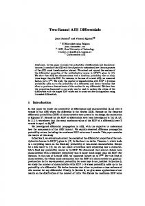
omitted group).6 Figure 1 (right scale) plots the

hospital differential estimated separately by year. This regression is similar to that in column one, except, the hospital RN dummy is interacted with year dummies. Estimates vary modestly from year to year. We are not willing to infer the presence of trends based on this evidence, although the decline since 1992 is intriguing. Results presented throughout the remainder of the paper utilize the pooled 1979-94 sample. Inferences based on estimates from subsets of the sample are identical. Since the nature of duties for RN jobs are likely to vary in and out of hospitals, a concern is that the measured hospital premium in part reflects occupational returns within the RN profession. The CPS does not allow us to distinguish staff RNs from, say, head nurses or specialists. The Sample Survey of Registered Nurses, however, contains this information.7 In a regression pooling the 1984, 1988, and 1992 SSRN and including similar variables to those used in Table 2 (but without occupational controls) we find that hospital RNs earn about 17.6 percent higher wages than non-hospital RNs, highly similar to our CPS estimate. When we include 4 separate occupational controls (administrator; head nurse/supervisor; staff, general duty, or private duty nurse; and specialist, with “other” position as the omitted group) the hospital differential increases slightly, to 20.0 percent. The hospital premium, therefore, does not appear to be driven by occupational differences between sectors. Although the major focus of the paper is the effect of hospital employment on earnings, other wage determinants presented in Table 2 are of interest. Black RNs receive wages 9.6 percent lower than white RNs. There is only a small difference in earnings between those employed by the public sector (federal, state, or local government) and those in the private sector. Marital status has only a marginal impact on wages, while male and female RNs earn similar wages, the latter result contrasting rather sharply with economy-wide evidence. Also, RNs who typically work less than 35 hours a week earn

6 The percentage difference in wages between hospital and practitioner’s office RNs is calculated from the log difference using [exp(0.127+0.078)-1]100, and similarly for nursing home RNs. 7The SSRN is a survey conducted by the U.S. Department of Health and Human Services, Public Health Services, Health Resource and Services Administration. The survey is mailed to a sample of currently licensed registered nurses and includes information on their education and work history. The SSRN provides roughly 25,000 observations per survey.

6

similar wages as those who work full-time, as

compared to the substantial part-time penalty in the

labor market as a whole (a similar result is obtained using the SSRN). Not shown in Table 2 are coefficients on the year dummies, reflecting the growth in real wages during the 1979-94 period following control for measured characteristics. Figure 1 (left scale) plots these coefficients for RNs, as well as similar coefficients from separate wage regressions for licensed practical nurses (LPNs) and a control group of female workers, the latter to reflect economy-wide movements in wage rates. The control group consists of college educated (i.e., years of schooling greater than or equal to 16) women in non-health related occupations.8 The figure shows that after accounting for measured characteristics, real and relative wages of RNs rose substantially over the period. An RN in 1993 earned .251 log points or 28.5 percent higher real wages than a similar RN in 1979. This growth was particularly rapid in the mid to late eighties, a period when reported nursing shortages were most severe. The RN wage index peaks in 1993 and falls rather sharply so that by 1994 the RN differential (as compared to a similar RN in 1979) had fallen to .204 log points.9 LPN wages followed a pattern similar to that for RNs, with wage growth slower in the late 1980s, but no decline in 1994 (annual sample sizes of LPNs are small). In contrast, the control group of college educated women experienced far more modest wage growth over the period, earning 7.6 percent higher real wages in 1994 than in 1979. Note that the rising wages for RNs relative to this control group is particularly noteworthy since there were widening skill and narrowing gender wage gaps over the period (Levy and Murnane, 1992). RN wage growth relative to male and female workers economy-wide was substantially higher (these results not shown). Longitudinal Evidence on the Hospital Wage Differential Estimates of the hospital premium from wage level equations may be biased owing to omitted measures of worker ability. If RN skills are not adequately measured by years of schooling, potential experience, and the other right-hand-side variables, and if omitted measures of human capital are

8The control group consists of the following broad occupational categories: executive, administrative, and managerial; professional specialty occupations; technicians and related support; sales, administrative support, and clerical; and service occupations (except protective and household services).

7

correlated with hospital employment, the hospital

coefficient in a wage level equation will be a biased

measure of the hospital premium. The hospital premium observed in our cross-sectional analysis is likely to reflect both compensating differentials for working conditions and unmeasured differences in ability correlated with hospital employment.10 This section attempts to determine the extent of such bias and to obtain longitudinal estimates of the hospital premium that account for unmeasured worker skills. The Wage Change Model Below, we modify equation 1 to account for unmeasured worker-specific skill differences fixed over a one year period. Letting χi represent the fixed effect on log wages for worker i and adding a time subscript t, the wage equation can be written as: (2)

J

H

Y

j =1

h=2

y=2

ln Wit = ∑ βjXijt + ∑θhINDiht + ∑τyYEARiy + χi + e' it

The error term in equation 1 is divided into an individual-specific quality component (χi) fixed over time (one year with our data) and a random, well behaved, component (ei'). If the omitted fixed effect, χ, is positively correlated with hospital employment (i.e., more able workers are located in hospitals), then estimates of the hospital wage premium from equation 2 are biased upward. Letting the symbol ∆ represent changes between adjacent years, a wage change equation will take the form (dropping the individual subscript i): (3)

J

H

D

j =1

h= 2

d =2

∆ ln Wd = ∑ βj∆Xjd + ∑θh∆INDhd + ∑ φdPERIODd + ∆e' d ,

where d indexes the time periods over which values are differenced, and PERIODd are dummies for the periods 1980/81 through 1994/95 (with 1979/80 the reference period). The major distinction between equations 3 and 2 is that the effects owing to unmeasured skills fall out, potentially allowing for unbiased estimates of the quality-constant hospital premium. For equation 3 to provide an unbiased measure of the hospital wage differential, sectoral switching is assumed to be exogenous and ability must be equally

9Result from the January 1996 edition of Employment and Earnings suggest this trend continued in 1995. Nominal median fulltime weekly earnings in 1995 were $695 (Table 39, page 205), while similar figures for 1994 and 1993 were $682 and $687, respectively. Thus real earnings for RNs have continued to fall in 1995.

8

valued at the margin by employers in both sectors

(Gibbons and Katz, 1992) and within a year’s

time.11 The estimate of the hospital premium is based on the change in wages for RNs who either switch into or out of hospital employment. If the hospital premium is due entirely to hospitals attracting higher skilled nurses, then the estimate of θ in the wage change equation should be close to zero, assuming marginal products are equivalent across sectors. The specification in equation 3 restricts the estimates in β to be symmetrical, so that the wage gains for hospital joiners are equivalent to the wage loss for hospital leavers, and those for hospital stayers are the same as those for non-hospital stayers.12 To relax this assumption, we subsequently include dummies for entry into a hospital, exit out of a hospital, and employment in a hospital in the first year. The coefficients on the joining and leaving variables measure the change in the log wage, as compared to staying in non-hospital or hospital employment, respectively. Although such a specification is less restrictive, the gain from reduced bias is offset in part by the loss in precision attaching to separate estimates based on the relatively smaller samples of hospital joiners and leavers. The Longitudinal Data Panel data are constructed from two sources (Appendix 1 provides a detailed description). First, multiple panels from the CPS ORG files for 1979/80 through 1993/94 are constructed by matching individuals in the same month in consecutive years. Second, the March CPS surveys for 1980 to 1995 are utilized. These surveys contain retrospective information on each worker's employment in the previous year, including the number of employers, the longest occupation and industry from the previous year, total earnings from all jobs last year, total weeks worked, and usual hours worked per week. The March

10 For an analysis of the econometric issues associated with longitudinal estimation, see Jakubson (1991). 11 If there is a comparative advantage among RN switchers such that hospital RNs are absolutely more productive in hospitals and absolutely less able than other RNs in, say, nursing homes then our interpretation does not follow. In that case the interpretation of the wage change results depend on the reason why people are switching industries. More generally, endogenous job and sectoral change may bias wage change estimates. Biases exist in both directions. For example, assume a hospital hires what turns out to be a low ability nurse at the going hospital wage. Once the mismatch is revealed, the nurse may move to a lower paying non-hospital job. This would bias upward longitudinal estimates of the hospital premium since we would observe a large wage decline. On the other hand, hospital nurses with an unusually low current wage, or an unusually high wage offer from a non-hospital employer, are most likely to voluntarily switch sectors, leading to a downward bias in hospital premium estimates. Insufficient information is available to model explicitly selection effects on job change.

9

surveys also contain information on current

earnings (on the primary job) and employment for a

quarter of the sample (the outgoing rotation groups). Those who are not outgoing in March provide information on current earnings in either April, May or June. Matching the March surveys with the ORG files for these months provides a nearly full sample of March CPS respondents for 1979/80 through 1994/95. In order to maximize sample size, the ORG and March panel data sets are combined, after eliminating from the ORG panel individuals surveyed in the months of March, April, May, or June (since they are already in the March panels). Because measurement error is a particular concern with longitudinal analysis, those with industry, occupation or earnings allocated (i.e., assigned) by the Census are deleted from the sample. The resulting panel data set for 1979/80 through 1994/95 contains data on 17,327 RNs, each observed in consecutive years. Of these, 11,887 (68.6 percent) were employed in a hospital in both years, 4,579 (26.4 percent) were employed outside of hospitals in both years, 338 (2.0 percent) switched to hospital employment, and 523 (3.0 percent) left hospital employment. It is important to note that there exists a bias toward zero in panel estimates using both the March and ORG data sets. Due to the method of measuring the initial (year 1) wage in the March surveys, a downward bias will be present to the extent that the wage in year 1 reflects in part the wage in the new employment setting and lowers the observed effect of changing industry. This is because the previous year’s wage is calculated from earnings on all jobs. RNs who, say, move to a hospital from a health practitioner’s office late in the first year, will report their longest industry last year as a health practitioner’s office. Their earnings from last year, however, will include the increase in wages due to hospital employment, and will bias downward the estimated effects of joining a hospital. The true wage effects of joining a hospital, therefore, are somewhat larger than suggested by the coefficient estimates. Calculations in Macpherson and Hirsch (1995, p. 458n ) suggest a bias of about 15 percent. The ORG panels, although not suffering from the downward bias described above, are more likely to contain measurement error in the industry (i.e., hospital) variable. The ORG panels are

12 Joiner and leaver coefficients may differ if, for example, slopes of wage profiles differ. A steeper wage profile implies

10

constructed from two separate surveys potentially

involving two separate interviewers and

interviewees, whereas the March data are collected at a single point in time. Measurement error lowers the signal to noise ratio and biases estimates of the effects of changing employment status toward zero. The BLS has examined the issue of occupation and industry coding in the CPS in some detail (Polivka and Rothgeb, 1993). Measurement error on industry assignment is rather modest, while that on detailed occupation is substantial. We are not concerned with measurement error on occupation, since we do not include occupational switchers in our analysis. Measurement error with respect to hospital (i.e., industry) employment appears less likely than for many other industries, given that respondents provide the name of their employer and coders assign the industry code. In order to gain additional insight into this issue, however, we turn to the 1992 SSRN, which for the first time asked RNs their employment setting (hospital, nursing home, etc.) the previous year and if they were employed by the same employer in the same position last year. This provides us with an independent measure of the extent of moving among RNs, one likely to have little measurement error. In the merged March/ORG panel, 2.0 percent of the sample were hospital joiners while 3.0 percent were hospital leavers. Analogous numbers from the SSRN (we define a switcher as an RN who says she changed employers and who has changed form hospital to non-hospital employment, or vice-versa) indicate that 1.9 percent were joiners and 3.2 percent were hospital leavers. Such a close correspondence suggests that measurement error associated with our hospital switching variable is small, thus increasing confidence in the paper’s principal results.13 Wage Change Results Table 3 presents the results of the wage change regression models.14 For comparison, the first column presents the hospital coefficient from a standard log wage regression run in levels using the year 2

smaller gains for entrants than losses for leavers. If hospitals tend to have flatter profiles than the non-hospital sector we may expect a larger premium to hospital joiners than loss to hospital leavers. 13Because the SSRN does not contain information about earnings or hours worked the previous year, wage change analysis is not possible. 14Individuals with top-coded (i.e., capped) earnings in either year are omitted from the wage change models, as are those with values of occupation, industry, or weekly earnings that have been allocated (i.e., assigned) by the Census. Hourly earnings calculated from March retrospective surveys for the previous year tend to be higher than current earnings from the CPS ORG for the second year, in part because the former includes earnings from all jobs. We include a dummy variable in the wage change equations designating whether the observation is from the March sample. This dummy yields a significant coefficient of about

11

information from the panel data set (non-hospital

employment is the omitted category). The second

column displays results from estimating equation 3 with a single variable for the change in hospital employment. The coefficient falls from 0.163 in the levels equation to 0.079 in the change equation, suggesting that approximately half of the hospital premium is due to higher unmeasured skills among hospital RNs. The hospital premium, following control for worker-specific skills, is about 8 percent. These results provide support for our hypothesis that a substantial portion of the observed hospital wage advantage reflects higher skills among hospital RNs. The March CPS data contain information on geographic mobility, and allow the effects of changing hospital employment to be estimated net of the effects of geographic mobility. Individuals in the ORG panels are by definition non-movers, since if they changed households they are no longer included in the CPS and cannot be in the panel. A mover is defined here as an individual who changed counties between years. The results in column 3 capture the interaction between the change in hospital employment and the decision to move. The dummy variable ∆HOSP*Mover is set to 1 (-1) when the individual both joins (leaves) a hospital and moves and 0 otherwise. The results indicate particularly large wage changes for those who move and change hospital status -- .158 log points (.071+.087) versus .071 for non-movers changing hospital status. RNs moving but not changing hospital status exhibit virtually no real wage gain (.008), as compared to those who do not move. We are reluctant to attach much weight to the large wage changes among RNs who both move geographically and change sector of employment, given the small number in this group (61) and the absence of wage changes for RNs who are geographic movers but do not change hospital status.15 The specification in column 4 provides estimates of the hospital premium that can differ depending on the sector from which RNs enter or exit. Three separate dummy variables are included for

-.07. When we estimate wage change models separately for each data set, we arrive at the same conclusions presented in the paper. 15One could argue that geographic movers may readily obtain information about what are relatively homogeneous job opportunities among a city's hospitals, while at the same time have poor information regarding the rather diverse job opportunities in practitioner offices, outpatient health facilities, and other sites where personal contacts and area-specific knowledge is essential. But if informational differences were driving the results, we should also observe geographic moving

12

changing hospital employment status (dummies are

included but not shown for three of the four types

of stayers). The results show that the “quality-adjusted” hospital premium, which averaged .079 (column 2), differs substantially across alternative types of employment. The hospital wage advantage is quite large (.175) when compared to alternative wages in health practitioners’ offices, whereas wage changes among RNs moving to or from employment in nursing homes or other industries are much smaller (.100 and .050). These results contrast with the cross-sectional differentials (Table 2) showing similar RN wages in health practitioners offices and nursing homes. A reasonable explanation for these results is that the large quality-adjusted wage differential between hospital and health practitioner RNs stems in no small part from what are more onerous hospital working conditions. In contrast, the smaller wage changes observed among RNs switching between hospitals and nursing homes or other employment sectors suggests that the hospital premium relative to these sectors derives primarily from nurse-specific ability differences. Direct evidence on industry-wide injury rates, although not providing a comprehensive measure of RN working conditions, indicates a very safe environment within practitioner offices, a relatively high-risk hospital environment, and dangerous employment within nursing home. In contrast to a 1992 economy-wide private sector rate of 3.6 injuries involving lost work time per hundred workers, employees in health practitioner offices (RNs and non-RNs) had an injury rate of only 0.8. The injury rate within hospitals was 4.1 and the rate within nursing and personal care facilities was 9.1, the latter being among the highest in the economy (U.S. Department of Labor, 1995, Table 1, p. 18-29).16 Table 4 shows the results of alternative wage change and wage level models relaxing the assumption of symmetry between leavers and joiners. The results in column 1 show that hospital joiners receive a premium of 8.4 percent relative to non-hospital stayers. Hospital leavers receive about 5.9 percent lower wages than hospital stayers. (HOSP=1 if in a hospital in year 1, so leavers have a wage change .061 log points less than hospital stayers and .085 log points less than non-hospital stayers.)

gains for the large sample of RN hospital stayers, and markedly lower gains (or losses) among the many non-hospital stayers who move. In fact, the data indicate little wage change among either group of geographic movers (these results not shown). 16Differences in rates for hospitals and nursing homes overstate risk differences for RNs, since many of the injuries within nursing homes are for nursing aides. In a ranking of industries based on back injuries involving lost work time, nursing and

13

Column 2 allows separate effects for geographic

movers. RNs who join a hospital but do not move

receive a wage gain of 7.4 percent, while those who both move and join a hospital receive a gain of 15.0 percent (the joint effect of HOSPJOIN and HOSPJOIN*Mover). Those who leave hospitals but do not move receive 5.2 percent lower wages, while those who also move receive an additional penalty of 9.8 percent. The results suggest rather modest asymmetry between the premium for joiners and penalty for leavers. A test of the null hypothesis that the coefficient for joiners is the same (in absolute value) as that for leavers fails to reject the null (F=0.648). Because the RN labor market was relatively tight over our sample period, most RNs who change employment do so voluntarily. This suggests that RNs change hospital employment to receive higher utility (wages, fringes, and job attributes). A hospital joiner, therefore, would receive a wage gain for changing jobs in addition to a premium for less pleasant working conditions. A leaver would receive a net utility gain for changing as well, but would see lower wages due to the improved working conditions of non-hospital employment. Thus, we would expect the loss to voluntary leavers to be lower (in absolute value) than the gain to joiners. Our results indicate that this is the case, although the difference is not statistically significant. The evidence on geographic movers in column 2 provides additional evidence on this point. Joiners and leavers who also move are more likely to be exogenous switchers since the decision by RNs to move geographically may be tied more closely to the move decision of a spouse than to their own job opportunities. In contrast to our finding of somewhat larger JOIN gains than LEAVE losses among switchers who do not move (.071 versus -.053), wage losses for leavers (-.156) are at least as large as the gain for joiners (.140) among hospital switchers who move.17

personal care facilities had the highest rate of any industry -- 3.29 per 100 workers annually versus 0.85 economy-wide (U.S. Department of Labor, 1995, p. 15). 17An alternative approach would be to estimate an endogenous switching model. We do not pursue this approach owing to a lack of adequate instruments correlated with hospital employment but not earnings.

14

The effects of unmeasured ability on

hospital premium estimates also can be

demonstrated using wage level estimation incorporating information from the subsequent or previous period.18 Columns 3 and 4 of Table 4 show wage regressions run in levels including dummies for the four employment transition groups to identify year one and year two wages. Included are dummies for first year hospital employment (HOSP), hospital employees in year 2 only (HOSPJOIN), and hospital employees in year 1 only (HOSPLEAVE), with non-hospital stayers the omitted comparison group. Column 3 uses the log real wage from year 1 as the dependent variable. The coefficient on HOSP (.195) indicates a 21.5 percent premium for RNs employed in hospitals in year 1, as compared to RNs who will be employed outside of hospitals in both years. The coefficient on HOSPJOIN indicates that those who subsequently will join a hospital in year 2 already earn a 3.4 percent premium in non-hospital employment in year 1. That is, RNs are rewarded for higher ability even before they join the hospital, and they select to switch to hospital employment even though they are paid more in non-hospital employment than other RNs with identical measured characteristics. The coefficient on HOSPLEAVE indicates that in year 1, wages for hospital RNs who will subsequently leave are already 6.9 percent lower than their hospital co-workers, even before they exit the hospital. This is consistent both with the ability sorting hypothesis in which less able RNs exit hospital employment, and a mobility model wherein hospital RNs receiving relatively low wages are most likely to leave. Using similar logic, the specification in column 4 uses the year 2 wage as the dependent variable. Those who have joined a hospital realize a 11.5 percent wage advantage compared to RNs in non-hospital employment, but 5.7 percent (calculated from the log differential .109-.168=-.059) less than RNs who were employed in hospitals in year 1. Those who have left hospital employment in year 2 receive 12.5 percent less than RNs remaining in hospital employment.

18 Although the estimation of this equation is in principle equivalent to that of the wage change equations, in practice the estimates differ, largely because of a differing structure of errors in levels and in changes (Mincer, 1983).

15

Additional Evidence on the Source of the

Hospital Wage Differential

Hospital Premiums Among Alternative Occupations We have presented evidence showing that RNs exhibit a sizable hospital wage premium, with roughly a third to a half reflecting higher (unmeasured) skills. The remainder results from what we believe are compensating differentials for working conditions. In this section we present an analysis for hospital and non-hospital workers in other occupations in order to gain insight into the nature of the RN premium. If hospital premiums of a magnitude similar to that received by RNs were evident among most hospital workers, it would support the thesis that there are substantial rents being shared by all hospital workers or that there exist work disamenities in hospitals for all workers and not just RNs. If these premiums decline substantially using wage change analysis, it would indicate that hospitals are matched with high quality workers in all occupations. Table 5 presents unadjusted log wage differentials between hospital and non-hospital workers, as well as estimated hospital premiums based on wage level and change equations. The occupations analyzed are health technologists and technicians (licensed practical nurses and radiologic and other technicians); health service occupations (including health aides and nursing aides); administrators and managers; secretaries, stenographers, and typists; and cleaning and building service occupations. Hospital differentials are evident among all occupations apart from secretaries, but are substantially smaller than those for RNs. Unlike the results for RNs, there is little evidence of a large compensating premium for higher skills among non-RN hospital workers, as seen by the rather small absolute changes in the premiums moving from wage level to wage change estimates. While selective matching on quality and a large hospital skill premium appear to be unique to RNs, non-skill related (i.e., longitudinal) hospital premiums of roughly 5-10 percent are realized by administrators and managers, cleaning occupation workers, and workers in health service occupations, a magnitude similar to that observed for RNs. In contrast, health technologists and secretaries display small longitudinal premiums on the order of 2-4 percent. Were the non-skill related premiums due to rent-sharing, we would expect the rents to be shared by most hospital workers, regardless of occupation, with lengthy queues of qualified applicants. This is not the case. 16

The comparison of hospital premiums

among RNs with those for other occupational

groups does not allow us to conclude decisively whether it is working conditions that account for the longitudinal premiums, absent more direct evidence on job disamenities and how they differ by occupation. What we can conclude from this analysis is that: 1) the magnitude of the RN hospital wage premium is substantially larger than for other occupational groups; 2) although a substantial share of the RN hospital premium is accounted for by high unmeasured skill among hospital nurses, positive sorting on skill is not important for other hospital occupations; and 3) a hospital wage advantage is evident among some but not all hospital workers, with such differentials believed to largely reflect unmeasured differences in working conditions between hospital and non-hospital employment. Hospital versus Non-Hospital Fringe Benefits The analysis to this point has considered only monetary compensation. One possibility is that hospitals pay higher wages in place of lower non-wage benefits. The March CPS supplements contain information on the availability of health insurance and pension plans. Row 1 of Table 6 shows that hospital employees have a higher probability of being offered a pension plan by their employer and of participating in this plan. While 52.2 percent of non-hospital RNs participate in pension plans (other than Social Security), 64.3 percent of hospital RNs participate. There is a similar result for health insurance. About three quarters of hospital RNs participate in an employer-sponsored health insurance program, while only 60 percent of non-hospital RNs have health insurance. Of those with insurance plans, similar proportions of hospital and non-hospital employers pay for at least part of the plan. These results show that, if anything, the hospital RN wage advantage understates the advantage in total compensation. Evidence on Nursing Skills: AFQT, Work Experience, Tenure, and Occupational Experience The CPS data set used in our analysis contains few direct measures of skill. Our panel analysis indicates that a substantial portion of the hospital wage premium is accounted for by unmeasured workerspecific skills. In this section, we utilize alternative data sets with evidence on cognitive ability, occupational experience, company tenure, and work experience among hospital and non-hospital RNs. If hospital RNs have higher productivity than RNs in other sectors, then we should observe corresponding differences in these measurable correlates of worker skill. 17

We first turn to the National Longitudinal

Survey of Youth (NLSY), which administered the

Armed Forces Qualifying Test (AFQT) in 1981, with individuals ranging in age from 16 to 24 at the time tested (scores were renormed in 1989). The AFQT, a widely used measure of individual premarket cognitive ability, is expressed as a percentile score and is based on the average of four tests included in the broader Armed Services Vocational Aptitude Battery. We use the 1991 cross-section of the NLSY, which contains data on 89 RNs, 72 employed in hospitals and 17 outside of hospitals. As seen in line 3 of Table 6, the mean AFQT percentile score for RNs is 65.1, substantially higher than the 50 percentile population average and the mean scores of 49.4 and 30.4 for LPNs and nursing aides, respectively (because the NLSY oversamples minorities, all figures are sample-weighted means). Consistent with expectations, we find that hospital RNs have a mean AFQT percentile score of 67.8, as compared to a mean of 53.2 for non-hospital RNs. Because aptitude test scores increase with age, we also ran a (sampleweighted) regression with AFQT on the left-hand-side, and a hospital dummy and dummies for age when the exam was administered included on the right-hand-side. The coefficient (standard error) on the hospital dummy was 13.49 (5.74), very similar to the 14.6 percentile difference without age adjustment. Although the observed difference in premarket aptitude between hospital and non-hospital RNs adds support to our ability hypothesis, ability differences measured by the AFQT account for at most a modest portion of the labor market skill advantage among hospital RNs. In a wage regression similar to that estimated in Table 2, we obtain an estimate of the hospital premium of .32 log points. Following control for AFQT, the estimated hospital advantage declines to .27. Although AFQT scores capture some of the skills valued in nursing markets, most of the worker-specific skills reflected in our longitudinal analysis involve abilities not measured by general aptitude tests.19 In lines 4a, 4b, 4c, and 4d of Table 6 evidence is provided on work experience, company tenure, and occupational tenure. We measure each of these proxies for market skill relative to years of potential experience (i.e., years since completing schooling), the variable used in our empirical work. In each of

19 Cawley et al. (1996) provide evidence from the NLSY that measured cognitive ability, while correlated with wages, explains relatively little of the variance in wages across individuals or over time. Neal and Johnson (1996), however, show that

18

these cases, hospital RNs display an advantage

relative to non-hospital RNs. Work experience data

on 378 RNs included in Survey of Income and Program Participation (SIPP) during 1990 indicate that hospital RNs have worked 92.7 percent of their potential years of experience, as compared to 85.9 percent among non-hospital RNs.20 The SIPP also contains information on tenure on the current job, and line 4b indicates that hospital RNs have spent 45 percent of their potential experience with their current employer, while non-hospital RNs spent 28 percent with their current employer. Turning next to CPS tenure supplements for January 1983, 1987, and 1991, hospital RNs are found to have spent 48 percent of their potential experience with their current employer, as compared to 29 percent among non-hospital RNs. Finally, occupational tenure (obtained from the same CPS surveys) relative to potential experience is high for RNs, accounting for 71 percent of potential years among hospital RNs and 64 percent among non-hospital RNs. The evidence provided in this section provides insight into some of the sources of unmeasured worker-specific skills reflected in our previous longitudinal estimates. Differences between hospital and non-hospital RNs in AFQT scores, work experience, and firm and occupational tenure reinforce our conclusion that unmeasured skills account for a significant portion of the hospital wage advantage. Union and Employer Size Effects on the Hospital Premium The panel results in Tables 3 and 4 were estimated without controlling for union status, since the March surveys do not ask retrospective questions on union coverage (the monthly ORG earnings files began including union status questions in January 1983). Because most unionized RNs are employed in hospitals or “other industries” (see Table 1), it is possible that the hospital premium is driven by differences in union status. The union premium for RNs is far too small, however, to account for much of the hospital premium (for evidence on the RN union premium, see Adamache and Sloan, 1982; Cain, et al., 1981 Feldman and Scheffler, 1982; or Hirsch and Schumacher, 1996). When we include the change in union status in a wage-change equation (using only the ORG panels from 1983/4 to 1993/4) the

differences in AFQT scores, absent control for schooling and other wage correlates, account for a sizable share of mean blackwhite wage differences.

19

coefficient on the change in hospital employment

falls only slightly, from 0.059 to 0.057, indicating

that little of the hospital premium is explained by union status. Consistent with prior evidence, we find that union premiums are smaller in hospitals than in non-hospital settings. Row 5 of Table 6 reveals a union-nonunion differential for RNs within hospitals of only 1.6 percent, as compared to a differential of 7.9 percent in non-hospital settings. Although the magnitude of the union premiums are small, this pattern is consistent with the economy-wide finding of smaller union premiums among large than among small employers (Mellow, 1983). Previous research has demonstrated a large economy-wide employer size effect (Brown and Medoff, 1989). Since hospitals tend to be large, part of the premium could be due to a similar phenomenon that occurs in other large firms or establishments. In work not shown, the effects of employer size in the nursing labor market are examined using the CPS benefit supplements for May 1979, 1983, and 1988. Our results show that there are large size effects and that the hospital premium falls substantially when controlling for either firm or establishment size. There remains a significant premium, however, of between 5 and 6 percent. Our result with respect to size does not explain the hospital premium, but suggests that the explanation may involve many of the same factors driving the economywide employer size effect. And evidence suggests some of the size premium reflects higher skilled workers among large employers (e.g., Brown and Medoff, 1989; Reilly, 1995). The Effects of Secondary Jobs Many RNs work in second jobs as nurses, some within hospitals and others outside of hospitals. The use of dual job information provides an alternative method for measuring the hospital wage differential, controlling for unmeasured person-specific skills. Whereas longitudinal analysis measures wage changes for given nurses changing sectors over time, the dual job analysis measures wage differences for given nurses taking jobs in different sectors during a single time period. Both methods control for worker fixed effects. The dual job comparison, however, is complicated by the fact that multiple job holders presumably face a maximum hours constraint on at least one of their jobs.

20The work experience variable in the SIPP was calculated as the number of years the individual worked at least 6 months in

20

The Sample Survey of Registered Nurses

(SSRN) asks licensed RNs if they hold more than

one nursing job for pay. If they respond yes, the survey then asks about their sector of employment, as well as hours worked per week, number of weeks worked per year, and annual earnings on the second job. Row 6 of Table 6 provides information from the SSRN. Approximately 10 percent of hospital RNs and 13 percent of non-hospital RNs work at second nursing jobs, 40 percent of these second jobs being in hospitals. Evident from row 6 is that wages in the primary job among dual job holders exceed the wages of single job holders, suggesting that dual job RNs tend to be highly motivated or skilled. Row 6 provides log wage differences between the secondary and primary jobs for the four possible groups of dual job holders. Letting P represent the primary job, S the secondary job, H a hospital job, and N a non-hospital job, we observe the log wage difference lnWs-lnWp for those whose (P,S) job pairs are HH, NN, NH, and HN. Sectoral stayers show little log wage difference between their secondary and primary jobs, -.01 for hospital and .01 for non- hospital stayers (owing to a high variance in second job wages, mean dollar wages are higher in secondary than in primary jobs for both groups). Among sectoral movers, we observe a .08 wage gain for hospital “joiners” (NH) and a -.10 wage change for hospital “leavers” (HN). We can impose symmetry on wage differences for sectoral stayers and changers by regressing lnWs-lnWp on ∆HOSP. This yields a coefficient (s.e.) on ∆HOSP of .092 (.012). This quality-adjusted hospital wage advantage estimate of .09, based on dual job sectoral changers, is highly similar to our earlier estimate of a .08 hospital advantage based on sectoral changers over time (Table 3). These results reinforce our earlier conclusion that a significant portion of the cross-sectional hospital premium reflects higher unmeasured skills among hospital nurses. Shift Differentials The results thus far suggest that roughly a third to a half of the cross-sectional hospital premium is due to omitted skill, while the remainder is a premium directly related to hospital employment, presumably due to compensating differences for job attributes. Information on job characteristics (such as shift worked, level of risk at the job, etc.) would allow this latter presumption to be tested more

that year. The SIPP data were kindly provided to us by Marjorie Baldwin.

21

directly. The 1985 and 1991 dual job supplements

to the May CPS survey contain work shift

information. To get a full sample (since only a quarter of the May survey, the outgoing rotation groups, contain information on earnings) these May supplements are merged with the full-year ORG data (workers not outgoing in May are outgoing in June, July, or August with earnings information in one of these months). These data allow us to estimate the shift premium and see how accounting for shift affects the hospital wage differential. The top panel of Table 7 shows mean wages and employment status by shift. About half of the sample works the daytime shift, and real wages are lowest for these RNs. Evening shift nurses earn, on average, 5.0 percent higher wages than day shift nurses, and night shift nurses earn 12.7 percent higher wages than day shift nurses. A large proportion of evening and night shift RNs are employed in hospitals, while few RNs in health practitioners’ offices work evenings or nights. Those working split or rotating shifts earn higher wages and are more likely to be employed in hospitals than day shift nurses. The second panel of Table 7 displays the effects of controlling for shift on hospital premium estimates. Without including the shift dummies, hospital RNs in this sample receive 21.0 percent higher wages than RNs in nursing homes and 31.7 percent higher wages than those employed in health practitioners' offices. When shift dummies are included, wage differences between RNs in the four industry classifications are lowered. While the estimated effects of controlling for shift are as expected, they are rather modest. The difference in earnings between hospital and nursing home RNs falls only slightly, consistent with the use of night shifts in both hospitals and nursing homes. The differential between hospital and health practitioners’ office RNs, where most hours are first shift, falls by more than three percentage points. Similarly, the differential between hospital RNs and RNs employed in other industries declines by about 2 percentage points. These results are consistent with the implication of Table 3 (column 4) that RNs in health practitioners’ offices earn lower wages primarily because of relatively pleasant working conditions, while nursing home RNs have lower wages due to lower skills. The magnitudes of the shift variables are interesting in their own right (for evidence from manufacturing, see Kostiuk, 1990). The shift premium to evening shift RNs is almost 4 percent, while for night shift RNs it is 11.6 percent. There is a small insignificant premium for working rotating or split 22

shifts over day shift. Although shift premiums are

significant wage determinants, they explain just

under 10 percent of the cross-sectional wage differential between hospitals and health practitioners’ offices (they explain a greater proportion of the non-ability component) and little of the differential between hospitals and nursing homes. Conclusions The purpose of this study has been to shed light on the sources of the large hospital wage premium realized by RNs. In cross sectional regressions, after controlling for measurable worker characteristics, there is an almost 20 percent wage difference between hospital and non-hospital RNs. Evidence on the receipt of health insurance and pension coverage suggests that the hospital compensation premium is even larger. Panel estimates from wage change models indicate that from a third to half of the hospital premium is due to hospitals attracting nurses of higher (unmeasured) ability. We conclude that much of the remaining differential is due to a compensating differential for differences in working conditions. Direct evidence on worker ability and job characteristics supports our interpretation. Hospital RNs have higher cognitive ability as measured by AFQT scores and have higher quality experience as measured by the ratios of total market experience, company tenure and occupational tenure to potential experience. A measurable job characteristic, shift work, accounts for roughly 10 percent of the cross-sectional hospital premium.21 Despite the importance of hospital employment among RNs, and the large magnitude of wage differences between hospital and non-hospital employment, there has been little study directed at uncovering the sources of the premium. Our study takes a step in this direction. Based on cross-sectional and panel analysis using large data sets constructed from various CPS files, we conclude that hospital RNs receive compensating differentials for higher unmeasured abilities and less pleasant working

21Close to 90 percent of young RNs (those below age 35) are found in hospitals, and many RNs move to non-hospital employment following their hospital experience and training. To the extent that RNs pay for general training in the form of lower wages, the hospital premium may be understated by our estimates, since hospital RNs receive not only higher wages and fringe benefits, but also training that increases their subsequent earnings. Separate estimates of the hospital premium for young and old RNs, however, indicates while the hospital differential rises slightly when compared to RNs in “other” industries (from .109 for those between the ages of 20 and 35, to .134 for those between the ages of 35 and 50, to .142 for those older than 50 ), it does not increase when compared to those in practitioner’s offices (.202 to .201 to .217 for the three age groups), and decreases slightly when compared to nursing homes (.211 to .179 to .160).

23

conditions. The analysis provides not only what we believe is an interesting study of compensating wage differentials, but also provides insight into the nature of wage determination in an important labor market.22 Our study also may shed light on the impact of evolving medical care patterns. Medical care services have begun to shift from in-patient hospital facilities to out-patient hospital and non-hospital settings. Indeed, a recent national commission study (the Pew Health Professions Commission) forecast that up to half the nation’s hospitals will close within five years and calculated a steep loss in nursing jobs based primarily on expected bed closures (Brider, 1996, provides an appropriately skeptical critique of the commission study). Whatever shifts do occur will not lead to RN employment loss proportional to the loss of hospital beds, but will decrease the share of total RN employment in hospitals. At first glance, the existence of a large hospital premium might lead to the expectation that the shift out of hospital employment will result in a significant wage decline for RNs. Despite the sizable hospital premium, the conclusion that RN wages and labor costs will decline substantially need not follow. First, our results show that as much as half of the hospital premium reflects unmeasured ability, with skill premiums received by high-ability RNs in or out of hospitals. Second, half or more of the hospital premium may result from less pleasant or more demanding working conditions in hospitals. To the extent that such working conditions are transferred to non-hospital settings, the compensating premium associated with these job disamenities will follow. Such a shift will increase relative RN wages in non-hospital settings and lower the measured hospital premium (its decline since 1992 is suggestive), while having only a modest effect on overall nursing labor costs.

22 Registered nurses comprise the third largest Census occupation among women, trailing secretaries and teachers.

24

0.3

0.2

0.25

0.18 0.16

0.2

0.14

0.15

0.12

0.1

0.1

0.05

0.08 0.06

0

0.04

-0.05

Hospital Differential

Adjusted Wage Index

FIGURE 1: RN and Control Group Wage Growth and Hospital Wage Differential, 1979-1994

0.02

-0.1

0 79 80 81 82 83 84 85 86 87 88 89 90 91 92 93 94

Year RN

LPN

Control

Hospital Differential

Data are from the CPS ORG files for 1979 through 1994. The series RN, LPN, and Control plot regression coefficients on year dummies (1979=0) from log wage equations run separately for each group. See text for a description of the control group, and variables included in the wage equations. The hospital differential series was calculated from an RN log-wage regression that included separate year dummies interacted with hospital employment (plus year dummies not interacted), thus providing annual estimates of the hospital premium for 1979-94.

25

TABLE 1 Means of Selected Characteristics for RNs by Employment Status

Hospital

Nursing Home

Practitioner’s Office

Other Industry

Real Wage

16.73

13.72

14.08

15.44

Years of Schooling

14.98

14.44

14.71

15.18

Age

37.26

44.29

41.06

41.94

Union Coverage

0.21

0.10

0.03

0.23

Percent Part-time

0.28

0.39

0.39

0.27

Public Employment

0.21

0.15

0.08

0.45

Metro Area (1 mill.+)

0.42

0.36

0.33

0.41

32,306

3,405

2,513

7,473

Sample Size

Data are from the CPS ORG files for the years 1979-1994. Real Wage is the mean wage measured in December 1994 dollars using the CPI-U. Practitioner’s Office includes nurses employed in the offices of physicians, dentists, chiropractors, optometrists and offices of health practitioners not elsewhere classified. Union coverage is based on the 1983-94 ORG files.

26

TABLE 2 Wage-Level Regression Results Coefficient Estimates Variable

(1)

(2)

Hospital

0.157 (0.003)

0.127 (0.004)

Practitioner’s Office

--

-0.078 (0.007)

Nursing Home

--

-0.059 (0.007)

Schooling

0.034 (0.001)

0.033 (0.001)

Potential Experience

0.014 (0.000)

0.013 (0.000)

Potential Experience Squared / 100

-0.028 (0.001)

-0.023 (0.001)

Black

-0.101 (0.006)

-0.102 (0.006)

Other Race

-0.043 (0.007)

-0.041 (0.007)

Hispanic

-0.049 (0.011)

-0.051 (0.011)

Female

-0.027 (0.007)

-0.028 (0.007)

Part-Time Status (hours worked per week < 35)

0.001 (0.003)

0.002 (0.003)

Public Employment

0.027 (0.004)

0.017 (0.004)

Married Spouse Present

0.014 (0.005)

0.014 (0.005)

Separated, Divorced, or Widowed

0.010 (0.006)

0.010 (0.006)

Sample Size

45,697

45,697

Data are from the CPS ORG files for the years 1979-94. Dependent variable is the log of the real wage. The omitted category in column 1 is all non-hospital employment; in column 2 “other industry” is omitted. Beginning in October 1985 the CPS identified 202 MSA/CMSAs; prior to that only 44 SMSAs are identified. For observations prior to October 1985 we include 3 size dummies and for observations after that time we include 7 size dummies. Other variables included in the regression are dummies for region (8), and year (shown in Figure 1). Potential Experience is measured as the minimum of age minus school minus six or age minus 16. Standard errors are in parentheses.

27

TABLE 3 Wage Level and Change Regression Results For Registered Nurses Dependent Variable ∆lnW ∆lnW ---

∆lnW --

HOSP

lnW 0.163 (0.005)

∆HOSP

--

0.079 (0.012)

0.071 (0.012)

--

∆HOSP*Mover

--

--

0.087 (0.046)

--

Mover

--

--

0.008 (0.014)

--

∆HOSP*Practitioner

--

--

--

0.175 (0.029)

∆HOSP*NurHome

--

--

--

0.100 (0.024)

∆HOSP*Other

--

--

--

0.050 (0.015)

Adj. R2

0.215

0.014

0.014

0.015

17,327

17,327

17,327

17,327

n

Data are from the combined ORG/March panels from 1979/80 through 1994/5. The regression in Column (1) is a levels regression with the log of the real wage in year 2 as the dependent variable. HOSP is a dummy variable equal to one if the individual is employed in a hospital in year 2. The regressions in columns (2), (3), and (4) are wage change regressions with the change in the log of the real wage as the dependent variable. ∆HOSP is the change in hospital employment status between years, and equals 1 (-1) if the individual joined (left) hospital employment between years and zero otherwise. Mover is defined as an individual who changed counties between years. The March 1985 survey question on moving differs from other years. These individuals are dummied out so that estimates presented in the table would not be affected. Other than the variables indicated, these regressions include the change in public sector status, the change in parttime status, the change in experience squared, year dummies, and a dummy designating those in the March panel. These regressions do not include the change in schooling, race, region, metropolitan area, or sex. Standard errors are in parentheses.

28

TABLE 4 Asymmetric Wage Level and Change Estimates of the Hospital Differential ∆lnW -0.024 (0.006)

Dependent Variable ∆lnW lnW1 -0.027 0.195 (0.006) (0.006)

lnW2 0.168 (0.005)

HOSPJOIN

0.081 (0.019)

0.071 (0.020)

0.033 (0.019)

0.109 (0.017)

HOSPLEAVE

-0.061 (0.015)

-0.053 (0.016)

-0.071 (0.015)

-0.134 (0.013)

--

0.069 (0.086)

--

--

HOSPLEAVE*Mover --

-0.103 (0.056)

--

--

Mover

0.006 (0.015)

--

--

HOSP

HOSPJOIN*Mover

--

See note to Table 3. Separate estimates of the hospital wage differential are provided based on the samples of RNs who are hospital joiners and leavers. HOSP = 1 if employment was in a hospital in year 1. The regression in column (3) is a levels regression with the log of the real wage in year 1 as the dependent variable and hospital status dummies are included - HOSP, HOSPJOIN, and HOSPLEAVE, with NONHOSP as the omitted group. Column (4) shows similar results using the wage in year 2 as the dependent variable. Standard errors are in parentheses.

29

TABLE 5 The Hospital Premium for Alternative Occupations Health Technologists

Health Service Occs

Administrators and Managers Secretaries

Cleaning Occupations

Unadjusted Log Wage Differential

0.065

0.178

0.140

-0.006

0.042

Regression Coefficients Hospital (from wage level eqn.)

0.063 (0.006)

0.152 (0.006)

0.050 (0.010)

-0.011 (0.007)

-0.003 (0.009)

0.037 (0.015)

0.103 (0.015)

0.052 (0.026)

0.016 (0.016)

0.121 (0.027)

12,484

16,382

65,591

44,349

18,961

Number of Switchers

578

646

252

459

223

%Hosp (in at least 1 year)

57.1

31.2

3.0

6.7

10.7

∆Hospital (from wage change eqn.) Sample Size

Data are from the combined ORG/March panels from 1979/80 through 1994/95. The unadjusted wage differential is the difference between the average log hospital wage and the average log non-hospital wage for each occupation. The coefficient on Hospital is the coefficient on a hospital dummy in a log wage regression. This regression also included as right-hand-side variables potential experience and its square, years of schooling; and dummies for race (2), Hispanic, sex, metropolitan area, marital status (2) part-time status, region (8), and year (15). The coefficient on ∆Hospital is the coefficient on a wage change equation that also included the changes in part-time status, public employment, experience squared, and year dummies.

30

TABLE 6 Additional Evidence on the Hospital Premium for Registered Nurses Hospital

Non-Hospital

1. Pension Coverage Plan Offered Participation

0.824 0.643

0.648 0.522

2. Health Insurance Participation All Paid Some Paid None Paid Family Covered

0.743 0.383 0.585 0.032 0.497

0.598 0.458 0.505 0.037 0.466

3. AFQT (Percentile score) 4. Measures of Market Experience a) Work Exp./Potential Exp. (SIPP) b) Company Tenure/Potential Exp. (SIPP) c) Company Tenure/Potential Exp. (CPS) d) Occupational Tenure/Potential Exp. (CPS)

N 12,002

12,002

67.8

53.2

89

0.927 0.448 0.475 0.709

0.859 0.278 0.294 0.635

378 378 2,663 2,763

5. Union Coverage Coeff. (s.e.)

0.016 (0.005)

0.076 (0.009)

34,797

6. Proportion Dual Job Single Job Holders, Primary Wage Dual Job Holders, Primary Wage RNs with Second Job in Hospital lnWs-lnWp RNs with Second Job in Nonhospital lnWs-lnWp

0.098 17.77 18.55

0.129 15.88 17.00

71,127 63,439 7,688 3,083

-0.012

0.078

-0.104

0.012

4,605

Data for rows 1 and 2 are from the March CPS surveys from 1980 through 1995. Participation is the percentage of employees who participate in employer-sponsored health insurance or pension plans. All Paid is the portion of health insurance plans paid in full by the employer, Some Paid is the proportion paid in part by the employer, and None Paid is the proportion paid in full by the employee. Family covered is the proportion of those with insurance that covers some or all of their family members. Row 3 displays the mean AFQT percentile score taken from the 1991 cross-section of the NLSY. Row 4a displays the ratio of actual work experience to potential experience taken from the 1990 Survey of Income and Program Participation. Row 4b is the ratio of company tenure to potential experience from the SIPP. Rows 4c and 4d show the ratio of company tenure and occupational tenure to potential experience and are taken from the CPS tenure supplements for January 1983, 1987, and 1991. The data in row 5 are regression coefficients on union coverage from a pooled log wage equation including separate hospital and non-hospital interaction terms. The data used are the 1983-94 CPS ORG files. Row 6 provides information on second jobs taken from the Sample Survey of Registered Nurses for 1984, 1988, and 1992. Proportion Dual Job is the portion of the sample who hold more than one position in nursing for pay. Primary Wage is the average real wage in the primary job (in December 1994 dollars), lnWp is the mean log wage in the primary job, and lnWs is the mean log wage in the secondary job.

31

TABLE 7 Evidence on the Shift Premium for Registered Nurses Descriptive Statistics Real Wage (1994 $) 17.21

Hospital 0.714

Nursing Home 0.068

Practitioner’s Office 0.051

All Shifts

n 1,242

Day Shift

703

16.60

0.619

0.067

0.083

Evening Shift

172

17.42

0.849

0.081

0.006

Night Shift

150

18.70

0.840

0.107

0.007

Rotating or Split Shift

129

17.70

0.876

0.031

0.008

Other Shift

88

18.39

0.761

0.045

0.023

Regression Results (1) 0.201 (0.025)

(2) 0.183 (0.025)

Nursing Home

0.010 (0.041)

0.007 (0.041)

Practitioner’s Office

-0.074 (0.046)

-0.066 (0.045)

Evening Shift

--

0.037 (0.027)

Night Shift

--

0.110 (0.028)

Rotating or Split Shift

--

0.046 (0.030)

Other Shift

--

0.043 (0.035)

Hospital

F ratio(4,983)

3.983

Data are from the May 1985 and 1991 dual job supplements to the CPS merged with the ORG files. Standard errors in parentheses. The F ratio tests the joint significance of the shift variables. A split shift is defined as "one consisting of two distinct periods each day," and a rotating shift is "one that changes periodically from days to evenings or nights." Other variables included are years of school, experience and its square; and dummies for region (8), public employment, gender, race (2), marital status (2), and year.

32

Appendix 1 Construction of Longitudinal Samples from the CPS ORG Files and the March CPS The CPS sample design is such that households are included in 8 surveys (rotation groups), beginning with 4 consecutive months in, followed by 8 months out, followed by 4 months in. Outgoing rotation groups 4 and 8 are asked earnings supplement questions (weekly earnings, hours, union status, etc.). The CPS contains household identification numbers (ID) and record line numbers, but not individual identifiers. Individuals potentially can be identified for the same month in consecutive years; that is, individuals in rotation 4 in year 1 can be matched to individuals in rotation 8 in year 2. The longitudinal ORG file was created in the following manner. Separate data files were created for males and females, and for pairs of years (rotation 4/1983 and rotation 8/1984, rotation 4/1984 and rotation 8/1985, etc.). Within each file, individuals were sorted as appropriate on the basis of ascending and descending household ID, year, and age. To be considered an acceptable matched pair, a rotation 8 individual had to be matched with a rotation 4 individual with identical household ID, identical survey month, and an age difference between 0 and 2 (since surveys can occur on different days of the month, age change need not equal 1). Several passes were necessary because a single household may contain more than one male or female pair. Checks were provided to insure that only unique matches were selected. For each rotation 8 individual, the search was made through all rotation 4 individuals with the same ID to make sure there was only 1 possible match; the file was resorted in reverse order and each selected rotation 4 individual was checked to insure a unique rotation 8 match. As uniquely matched pairs were identified they were removed from the work file. Incorrect changes in the variables marital status, veteran status, race, and education (e.g., a change in schooling other than 0 or 1, a change from married to never married, etc.) were used to delete "bad" observations in households where there were multiple observations and ages too close to separate matched pairs. Several passes at the data were made. In households where two pairs of individuals could be separated based on a 1 year but not the 0 to 2 year age change, a 1 year criterion was used. If a unique pair could not be identified based on these criteria, they were not included in the data set (e.g., four observations with two identical pairs, or three individuals with two possible matches using the 0 to 2 age change criterion). There are several reasons why matches cannot be made or that individual worker pairs are not included in the CPS ORG panel. The principal reasons are if a household moves (thus changing the household ID), if an individual moves out of a household, if a worker becomes self employed, if an individual drops out of the labor market or fails to meet other sample selection criteria, or if the Census is unable to reinterview a household and/or receive information on the individual. Inclusion rates for the entire CPS ORG panel are just under two-thirds of employed wage and salary workers in any year; rates are somewhat lower in our RN sample. Peracchi and Welch (1995) analyze attrition rates among matched March CPS files and conclude that age is the most important determinant of a successful match. Other factors that lessen match probabilities are poor health, low schooling, and not a household head, while sex and race are unimportant match predictors following control for other factors. Finally, sample sizes are reduced further to roughly half the normal size for the 1984/5 panel and to one-quarter for 1985/6. This is the result of a CPS test sample from July-September 1985 that implemented new population weights. Rotation 4 households interviewed in July 1984 through September 1985 were not reinterviewed a year later in 1985 and 1986. The March CPS longitudinal file is a retrospective panel. All rotation groups in March are asked information about earnings, weeks worked, and hours worked last year, and occupation and industry on the longest job held last year. A quarter sample in March (the ORGs) are asked current earnings, hours, etc. The entire March sample is matched to their earnings supplement records in their outgoing month, either March, April, May, or June. These records were matched initially on the basis of household ID and line number, followed by checks on changes in sex and age to insure an accurate match. The March retrospective panel is about three-quarters the size of a March sample based on the presence of earnings last year (and other typical variables). Losses are due to households moving, individuals leaving the household, changing employment status (i.e., leaving the labor force or shifting to self employment), changing line number, a failure to be reinterviewed, and missing hours or weekly earnings in the earnings supplement among employed wage and salary workers who are otherwise matched. The March CPS file and CPS ORG panel files are merged, with the March-June records deleted from the CPS ORG files to prevent double counting.

33

References Adamache, Killard W., and Frank A. Sloan. 1982. "Unions and Hospitals, Some Unresolved Issues." Journal of Health Economics, Vol. 1, No. 1 (May), pp. 81-108. Booton, Lavone A. and Julia I. Lane. 1985. "Hospital Market Structure and the Return to Nursing Education." Journal of Human Resources, Vol. 20, No. 2 (Spring), pp. 184-96. Brider, Patricia. 1996. “Huge Job-Loss Projections Shock Health Professions.” American Journal of Nursing, Vol. 96, No. 1 (January), pp. 61, 64. Brown, Charles, and James Medoff. 1989. "The Employer Size-Wage Effect." Journal of Political Economy, Vol. 97, No. 5 (October), pp. 1027-59. Cain, Glen G., Brian E. Becker, Catherine G. McLaughlin and Albert E. Schwenk. 1981. "The Effect of Unions on Wages in Hospitals." in Research in Labor Economics, edited by Ronald Ehrenberg, volume 4: 191-320, Greenwich, CT, JAI Press Inc. Cawley, John, Karen Conneely, James Heckman, and Edward Vytlacil. 1996. "Measuring the Effects of Cognitive Ability." National Bureau of Economic Research Paper 5645 (July). Curran, Connie R., Ann Minnick and Joan Moss. 1987. "Who Needs Nurses?" American Journal of Nursing, Vol. 87, No. 3 (March), pp. 444-47. DuMond, J. Michael, Barry T. Hirsch and David A. Macpherson. 1996. “Wage Differentials Across Labor Markets and Workers: Does Cost of Living Matter?” Florida State University, Department of Economics, Working Paper 96-08-1. Feldman, Roger, and Richard Scheffler. 1982. "The Union Impact on Hospital Wages and Fringe Benefits." Industrial and Labor Relations Review, Vol. 35, No. 2 (January), pp. 196-206. Gibbons, Robert, and Lawrence F. Katz. 1992. "Does Unmeasured Ability Explain Inter-Industry Wage Differentials?" Review of Economic Studies, Vol. 59, No. 3 (July), pp. 515-35. Groshen, Erica L., and Alan B. Krueger. 1990. "The Structure of Supervision and Pay in Hospitals." Industrial and Labor Relations Review, Vol. 43, No. 3 (February), pp. 134S-46S. Hirsch, Barry T., and David A. Macpherson. 1996. Union Membership and Earnings Data Book: Compilations from the Current Population Survey (1996 Edition). Washington, D.C.: Bureau of National Affairs. Hirsch, Barry T., and Edward J. Schumacher. 1995. "Monopsony Power and Relative Wages in the Labor Market for Nurses." Journal of Health Economics, Vol. 14, No. 4 (November), 443-76. Hirsch, Barry T., and Edward J. Schumacher. 1996. “Union Wages, Rents, and Skills in Health Care Labor Markets.” East Carolina University, Department of Economics, Working Paper 9603 (March). Hwang, Hae-shin, W. Robert Reed, and Carlton Hubbard. 1992. “Compensating Wage Differentials and Unobserved Productivity.” Journal of Political Economy, Vol. 100, No. 4 (August), pp. 835-58.

34

Jakubson, George. 1991. “Estimation and Testing of the Union Wage Effect Using Panel Data.” Review of Economic Studies, Vol. 58, No. 5 (October), pp. 971-91. Kostiuk, Peter F. 1990. “Compensating Differentials for Shift Work.” Journal of Political Economy, Vol. 98, No. 5, pt. 1 (October), pp. 1054-75. Lehrer, Evelyn L., William D. White, and Wendy B. Young. 1991. "The Three Avenues to a Registered Nurse License: A Comparative Analysis." Journal of Human Resources, Vol. 26, No. 2 (Spring), pp. 262-79. Levy, Frank, and Richard J. Murnane. 1992. “U.S. Earnings Levels and Earnings Inequality: A Review of Recent Trends and Proposed Explanations.” Journal of Economic Literature, Vol. 30, No. 3 (September), pp. 1333-81. Link, Charles R. 1988. "Returns to Nursing Education: 1970-84." Journal of Human Resources, Vol. 23, No. 3 (Summer), pp. 372-87. Macpherson, David A., and Barry T. Hirsch. 1995. ”Wages and Gender Composition: Why Do Women’s Jobs Pay Less?” Journal of Labor Economics, Vol. 13, No. 3 (July), pp. 426-71. Mellow, Wesley. 1983. “Employer Size, Unionism, and Wages.” In Research in Labor Economics, Supplement 2, ed. Ronald Ehrenberg, 253-82, Greenwich, CT, JAI Press Inc. Mincer, Jacob. 1983. "Union Effects: Wages, Turnover, and Job Training." In Research in Labor Economics, Supplement 2, ed. Ronald Ehrenberg, 217-52, Greenwich, CT, JAI Press Inc. Neal, Derek A. and William R. Johnson. 1996. "The Role of Premarket Factors in Black-White Wage Differences," Journal of Political Economy, Vol. 104, No. 5 (October), pp. 869-95. Peracchi, Franco and Finis Welch. 1995. "How Representative are Matched Cross Sections? Evidence from the Current Population Survey." Journal of Econometrics, Vol. 68, No. 1 (July), pp. 153-80. Polivka, Anne E. and Jennifer M. Rothgeb. 1993. “Overhauling the Current Population Survey: Redesigning the Questionnaire.” Monthly Labor Review, Vol. 116 (September), pp. 10-28. Reilly, Kevin T. 1995. “Human Capital and Information: The Employer Size-Wage Effect.” Journal of Human Resources, Vol. 30, No. 1 (Winter), pp. 1-18. U.S. Department of Labor, Bureau of Labor Statistics. 1995. Occupational Injuries and Illnesses: Counts, Rates, and Characteristics, 1992, Washington: GPO, April. U.S. Department of Labor. 1993. Selected Characteristics of Occupations Defined in the Revised Dictionary of Occupational Titles, Washington: GPO. Weiss, Andrew. 1990. Efficiency Wages: Models of Unemployment, Layoffs, and Wage Dispersion, Princeton: Princeton University Press.

35