Data-Dependent Iteration. Soonhoi Ha, Student Member, IEEE, and Edward A. Lee, Member, IEEE. Abshct- Scheduling of data-flow graphs onto parallel pro-.
1225
IEEE TRANSACTIONS ON COMPUTERS, VOL. 40, NO. 11, NOVEMBER 1991
Compile-Time Scheduling and Assignment of Data-Flow Program Graphs with Data-Dependent Iteration Soonhoi Ha, Student Member, IEEE, and Edward A. Lee, Member, IEEE
Abshct- Scheduling of data-flow graphs onto parallel processors consists in assigning actors to processors, ordering the execution of actors within each processor, and firing the actors at particular times. Many scheduling strategies do at least one of these operations at compile time to reduce run-time cost. In this paper, we classify four scheduling strategies: 1) fully dynamic, 2) static-assignment, 3) self-timed, and 4) fully static. These are ordered in decreasing run-time cost. Optimal or near-optimal compile-time decisions require deterministic, data-independent program behavior known to the compiler. Thus, moving from strategy 1) toward 4) either sacrifices optimality, decreases generality by excluding certain program constructs, or both. This paper proposes scheduling techniques valid for strategies 2), 3), and 4). In particular, we focus on data-flow graphs representing data-dependent iteration; for such graphs, although it is impossible to deterministically optimize the schedule at compile time, reasonable decisions can be made. For many applications, good compile-time decisions remove the need for dynamic scheduling or load balancing. We assume a known probability mass function for the number of cycles in the data-dependent iteration and show how a compile-time decision about assignment and/or ordering as well as timing can be made. The criterion we use is to minimize the expected total idle time caused by the iteration; in certain cases, this will also minimize the expected makespan of the schedule. We will also show how to determine the number of processors that should be assigned to the data-dependent iteration. The method is illustrated with a practical programming example, yielding preliminary results that are very promising. Index Terms- Data flow, data-dependent iteration, parallel processors, parallelizing compilers, quasi-static scheduling, scheduling.
I. INTRODUCTION
A
data-flow representation is suitable for programming multiprocessors because parallelism can be extracted automatically from the representation [l], [2]. Each node, or actor, in a data-flow graph represents a task to be executed according to the precedence constraints represented by arcs, which also represent the flow of data. Nodes in a data-flow graph are to be scheduled in such a way as to achieve the fastest execution from a given multiprocessor architecture. We make no assumption here about the granularity of the data-flow graph. The proposed techniques are valid both for fine-grain and large-grain. Manuscript received May 15, 1989; revised February 6, 1990. This work was supported by the Defense Advanced Research Projects Agency. The authors are with the Department of Electrical Engineering and Computer Sciences, University of California at Berkeley, Berkeley, CA 94720. IEEE Log Number 9102631.
Scheduling of parallel computations consists in assigning actors to processors, ordering the actors on each processor, and specifying their firing time, each of which can be done either at compile time or at run time. Depending on when a particular operation is done, we define four classes of scheduling. The first is fully dynamic, where actors are scheduled at run-time only. When all input operands for a given actor are available, the actor is assigned to an idle processor at run time. The second type is static allocation, where an actor is assigned to a processor at compile time and a local run-time scheduler invokes actors assigned to the processor. In the third type of scheduling, the compiler determines the order in which actors fire as well as assigning them to the processors. At run-time, the processor waits for data to be available for the next actor in its ordered list and then fires that actor. We call this selftimed scheduling because of its similarity to self-timed circuits. The fourth type of scheduling is fully static; here the compiler determines the exact firing time of actors, as well as their assignment and ordering. This is analogous to synchronous circuits. As with most taxonomies, the boundaries between these categories are not rigid. We can give familiar examples of each of the four strategies applied in practice. Fully dynamic scheduling has been applied in the MIT static data-flow architecture [lo], the LAU system, from the Department of Computer Science, ONERNCERT, France [3S], and the DDMl [9]. It has also been applied in a digital signal processing context for coding vector processors, where the parallelism is of a fundamentally different nature than that in data-flow machines [23]. A machine that has a mixture of fully dynamic and static assignment scheduling is the Manchester data-flow machine [39]. Here, 15 processing elements are collected in a ring. Actors are assigned to a ring at compile time, but to a PE within the ring at run time. Thus, assignment is dynamic within rings, but static across rings. Examples of static-assignment scheduling include many data-flow machines [37]. Data-flow machines evaluate dataflow graphs at run time, but a commonly adopted practical compromise is to allocate the actors to processors at compile time. Many implementations are based on the tagged-token concept [2] for example TI’S data-driven processor (DDP) executes Fortran programs that are translated into data-flow graphs by a compiler [SI using static assignment. Another example (targeted at digital signal processing) is the NEC uPD7281 [SI. The cost of implementing tagged-token architectures has
0018-9340/91$01.00 0 1991 IEEE
1226
IEEE TRANSACTIONS ON COMPUTERS, VOL. 40, NO. 11, NOVEMBER 1991
recently been dramatically reduced using an “explicit token store” [34]. Another example of an architecture that assumes static assignment is the proposed “argument-fetching data-flow architecture” [151, which is based on the argument-fetching data-driven principle of Dennis and Gao [111. When there is no hardware support for scheduling (except synchronization primitives), then self-timed scheduling is usually used. Hence, most applications of today’s generalpurpose multiprocessor systems use some form of self-timed scheduling, using for example CSP principles [19] for synchronization. In these cases, it is often up to the programmer, with meager help from a compiler, to perform the scheduling. A more automated class of self-timed schedulers targets wavefront arrays [24]. Another automated example is a dataflow programming system for digital signal processing called Gabriel that targets multiprocessor systems made with programmable DSP’s [28]. Taking a broad view of the meaning of parallel computation asynchronous digital circuits can also be said to use self-timed scheduling. Systolic arrays, SIMD (single instruction, multiple data), and VLIW (very large instruction word) computations [ 131 are fully statically scheduled. Again taking a broad view of the meaning of parallel computation, synchronous digital circuits can also be said to be fully statically scheduled. As we move from strategy 1 to strategy 4, the compiler requires increasing information about the actors in order to construct good schedules. However, assuming that information is available, the ability to construct deterministically optimal schedules increases. To construct an optimal fully static schedule, the execution time of each actor has to be known; this requires that a program have only deterministic and data-independent behavior [25], [26]. Constructs such as conditionals and data-dependent iteration make this impossible and realistic 1/0 behavior makes it impractical. The concept of static scheduling has been extended to solve some of these problems, using a technique called quasi-static scheduling [27]. In quasi-static scheduling, some firing decisions are made at run time, but only where absolutely necessary. Self-timed scheduling in its pure form is effective for only the subclass of applications where there is no datadependent firing of actors and the execution times of actors do not vary greatly. Signal processing algorithms, for example, generally fit this model [25], [26]. The run-time overhead is very low, consisting only of simple handshaking mechanisms. Furthermore, provably optimal (or close to optimal) schedules are viable. As with fully static scheduling, data-dependent behavior is excluded if the resulting schedule is to be optimal. Again, quasi-static scheduling solves some of the problems, but data-dependent iteration has been out of reach except for certain special cases. Static-assignment scheduling is a compromise that admits data dependencies, although all hope of optimality must be abandoned in most cases. Although static-assignment scheduling is commonly used, compiler strategies for accomplishing the assignment are not satisfactory. Numerous authors have proposed techniques that compromise between interprocessor communication cost and load balance [33], [6], [40], [31], [12], [30]. But none of these consider precedence relations between
actors. To compensate for ignoring the precedence relations, some researchers propose a dynamic load balancing scheme at run time [22], [4], [21]. Unfortunately, the cost can be nearly as high as fully dynamic scheduling. Others have attempted with limited success to incorporate precedence information in heuristic scheduling strategies. For instance, Chu and Lan use very simple stochastic computation models to derive some principles that can guide heuristic assignment for more general computations [7]. Fully dynamic scheduling is most able to utilize the resources and fully exploit the concurrency of a data-flow representation of an algorithm. However it requires too much hardware and/or software run-time overhead. For instance, the MIT static data-flow machine [lo] proposes an expensive broad-band packet switch for instruction delivery and scheduling. Furthermore, it is not usually practical to make globally optimal scheduling decisions at run time. One attempt to do this by using static (compile-time) information to assign priorities to actors to assist a dynamic scheduler was rejected by Granski et al., who conclude that there is not enough performance improvement to justify the cost of the technique P81. In view of the high cost of fully dynamic scheduling, static-assignment and self-timed are attractive alternatives. Self-timed is more attractive for scientific computation and digital signal processing, while static-assignment is more attractive where there is more data dependency. Consequently, it is appropriate to concentrate on finding good compiletime techniques for these strategies. In this paper we propose a way to schedule a data-dependent iteration for general cases with the assumption that the probability distribution of the number of cycles of the iteration is known or can be approximated at compile time. The technique is not optimal except in certain special cases, but it is intuitively appealing and computationally tractable. In the next section, we set the context by explaining what we mean by data-dependent iteration, and explaining precisely the problem we are solving. A complete compiler using this solution also needs other scheduling techniques from the literature, as explained. In Section 111, we introduce the notion of “assumed” execution time for a data-dependent iteration. Once the scheduler “assumes” an execution time for the iteration, it can construct a static schedule containing the iteration. The question addressed in this section is, what should the assumed execution time be? The answer is not the expected execution time, as one might expect. Instead, the answer depends on the number of processors devoted to the iteration relative to the total number of processors. In Section IV we explain how to decide how many processors to devote to the iteration. Section V describes the technique applied to a real programming example from graphics. Section VI explains precisely why the proposed technique is not optimal, except under unrealistic assumptions, but also why we should expect good performance. Through Section VI we have assumed “quasistatic” execution, which requires global synchronization of the processors. In Section VII, we show that the method applies much more broadly to self-timed and static-assignment scheduling.
1227
HA AND LEE COMPILE-TIME SCHEDULING AND ASSIGNMENT OF DATA-FLOW PROGRAM GRAPHS
11. DATA-DEPENDENT ITERATION In data-dependent iteration, the number of iteration cycles is determined at run time and cannot be known at compile time. Two possible data-flow representations for data-dependent iteration are shown in Fig. 1 [27]. The numbers adjacent to the arcs indicate the number of tokens produced or consumed when an actor fires [25]. In Fig. l(a), since the up-sample actor produces X tokens each time it fires and the iteration body consumes only one token when it fires, the iteration body must fire X times for each firing of the up-sample actor. In Fig. 1(b), the number of iterations need not be known prior to the commencement of the iteration. Here, a token coming in from above is routed through a “select” actor into the iteration body. The “D” on the arc connected to the control input of the “select” actor indicates an initial token on that arc with value “false.” This ensures that the data coming into the “F’ input will be consumed the first time the “select” actor fires. After this first input token is consumed, the control input to the “select” actor will have value “true” until the function t(.) indicates that the iteration is finished by producing a token with value “false.” During the iteration, the output of the iteration function f ( . ) will be routed around by the “switch” actor, again until the test function t ( . )produces a token with value “false.” There are many variations on these two basic models for data-dependent iteration. For simplicity, we will group the body of a data-dependent iteration into one node, and call it a data-dependent iteration actor. In other words, we assume a hierarchical data-flow graph. In Fig. l(a), the “iteration body” actor consists of the up-sample, data-dependent iteration, and down-sample actors. The data-dependent iteration actor may consist of a subgraph of arbitrary complexity and may itself contain data-dependent iterations. In Fig. 1(b), everything between the “select” and the “switch,” inclusive, is the data-dependent iteration actor. In both cases, the data-dependent iteration actor can be viewed as an actor with a stochastic run time, but unlike atomic actors, it can be scheduled onto several processors. Although our proposed strategy can handle multiple and nested iteration, for simplicity all our examples will have only one iteration actor in the data-flow graph. The method given in this paper can be applied to both kinds of iteration in Fig. 1 identically. There is, however, an important difference between them. In Fig. l(b), each cycle of the iteration depends on the previous cycle. There is a recurrence that prevents simultaneous execution of successive cycles. In Fig. l(a), there is no such restriction, unless the iteration body itself contains a recurrence. For the purposes of this paper, we will simply assume that successive cycles of the iteration must be executed sequentially. An extension that handles overlapped cycles will be reported in a separate paper. The proposed scheme has two components. First, the compiler must determine which processors to allocate to the datadependent iteration actor. These will be called the iteration processors, and the rest will be called noniteration processors. Second, the data-dependent iteration actor is optimally assigned an assumed execution time, to be used by the scheduler. In other words, although its run time will actually be random,
I-
I
Fig. 1. Data-dependent iteration can be represented using the either of the data-flow graphs shown. The graph in (a) is used when the number of iterations is known prior to the commencement of the iteration, and (b) is used otherwise
the scheduler will assume a carefully chosen deterministic run time and construct the schedule accordingly. The assumed run time is chosen so that the expected total idle time caused by the difference between the assumed and actual run times is minimal. It is well known that locally minimizing idle time fails to minimize expected makespan, except in certain special cases. (The makespan of the schedule is defined to be the time from the start of the computation to when the last processor finishes.) We will discuss these special cases and argue that the strategy is nonetheless promising, particularly when combined with other heuristics. Using the assumed execution time, a fully static schedule is constructed. When the program is run, the execution time of data-dependent actors will probably differ from the assumption, so processors must be synchronized. If all processors are synchronized together, using for example a global “enable” line, then we say the execution is quasi-static. It is not fully static because absolute firing times depend on the data. If processors are pairwise synchronized, then the execution is self-timed or static-assignment, depending on whether ordering changes are permitted. The assumed execution time and the number of processors devoted to the iteration together give the scheduler the information it needs to schedule all actors around the data-dependent iteration. It does not address, however, how to schedule the data-dependent iteration itself. We will not concentrate on this issue because it is the standard problem of statically scheduling a periodic data-flow graph onto a set of processors [25]. Nonetheless, it is worth mentioning techniques that can be used, To reduce the computational complexity of scheduling and to allow any number of nested iterations without difficulty, blocked scheduling can be used. In blocked scheduling, all iteration processors are synchronized after each cycle of the iteration so that the pattern of processor availability is flat before and after each cycle (meaning that all processors become available for the next cycle at the same time). If the scheduling is fully static, then this can be accomplished by padding with no-ops so that each processor finishes a cycle at the same time. The wasted computation can be reduced using advanced techniques such as retiming
.
II
1228
IEEE TRANSACTIONS ON COMPUTERS, VOL. 40, NO. 11, NOVEMBER 1991
or loop winding’ [29], [17]. In these techniques, several cycles of an iteration are executed in parallel to increase the overall throughput. For blocked scheduling, the objective is to minimize the makespan of one cycle. Throughput can also be improved using optimal periodic scheduling strategies, such as cyclostatic scheduling [36]. The proposal below applies regardless of the method used, but in all our illustrations we assume blocked scheduling. We similarly avoid specifics about how the scheduling of the overall data-flow graph is performed. Our method is consistent with simple heuristic scheduling algorithms, such as Hu-level scheduling [20], as well as more elaborate methods that attempt, for example, to reduce interprocessor communication costs. Broadly, our method can be used to extend any deterministic scheduling algorithm (based on execution times of actors) to include data-dependent iteration.
pattern simply defines the relative times at which processors become free after the iteration. For now, assume this pattern is strictly enforced by some global synchronization mechanism, regardless of the number of iteration cycles actually executed at run time. This will force either the iteration processors or the noniteration processors to be idle, depending on whether the iteration finishes early or late. This constraint is precisely what we mean by “quasi-static’’ scheduling of data-dependent iterations. It is not strictly static, in that exact firing times are not given at compile time, but relative firing times are enforced. Consider the case where the assumed number z is exactly correct. Then no idle time exists on any processor (Fig. 2(a)). Otherwise, the noniteration processors will be idled if the iteration takes more than z cycles (Fig. 2(b)), or else the iteration processors will be idled (Fig. 2(c)). Our strategy is to select z to minimize the expected idle time on all processors for a given number of iteration processors. Let p ( i ) be the probability mass function of the number of iteration cycles confined within MIN and MAX. For a fixed assumed z the expected idle time t l ( z ) on the iteration processors is
111. THE ASSUMEDEXECUTION TIME To schedule the actors around the data-dependent iteration actor at compile time, it is necessary to assign some fixed execution time to the data-dependent iteration actor. Since the number of cycles of the iteration to be executed is not known at compile time, we have to assume a number. The first guess might be to simply assume the expected execution time, which can be approximated using methods proposed by Martin and Estrin [32], but this will often be far from optimal. In fact, the assumed number should depend on the ratio of the number of iteration processors to the total number of processors. When the actual execution time differs from the assumed run time, some processors will be idled as a consequence. Our strategy is to find the assumed run time that minimizes the expected value of this idle time. We make the bold assumption that the probability distribution of the number of cycles of the iteration actor is known or can be approximated at compile time. Let the number of cycles of an iteration be a random variable I with known probability mass function p ( i ) . Denote the minimum possible value of I by MIN and the maximum by MAX. MAX need not be finite. In this section, we assume that we have already allocated somehow the number N of processors to the data-dependent iteration actor. How to allocate the number of processors will be addressed in the next section. If the total number of the processors is T , the number of noniteration processors is T - N . Let the assumed execution time of the data-dependent iteration actor be t. For the time being we restrict t to multiples of the execution time of one cycle of the iteration. If the execution time of a cycle is T , then z = t / denotes ~ the assumed number of cycles of the iteration. At run time, for each invocation of the iteration actor, there are three possible outcomes: the actual number i of cycles of the iteration is equal to, greater than, or less than z. These cases are displayed in Fig. 2. In order for the scheduler to resume static scheduling after the iteration is complete, it must know the “pattern of processor availability.” As indicated in Fig. 2, this ‘As a possibly interestingside issue, it does not appear to have been pointed out in the literature that retiming is simply a data-flow perspective on loop winding, so the techniques are in fact equivalent.
X
tl(.)
p ( i ) ( z- i).
= NT
(1)
2=MIN
The expected idle time t2(z)on the noniteration processors is MAX
t2(z)= (T - N)T
p(i)(Z - x).
(2)
2=x+1
+
The total expected idle time t ( z )is t ( z )= t l ( z ) tz(z).The optimal value of z minimizes this quantity. From this we can get that
t ( z )- t ( z + 1) = -NT
X
p(i)
+ (T - N ) T
z=MIN
MAX
p(i) G X + l
MAX
= -NT+TT
p(i).
(3)
2=x+l Similarly, MAX
t ( z )- t ( z - 1) = N T - TT
p(i).
(4)
Z=X
The optimal z will satisfy the following two inequalities: t ( z ) - t ( z 1) 5 0 and t ( z ) - t ( z - 1) 5 0. Since T is positive, from (3) and (4),
+
MAX
N
P(4
z=x+l
Ir 5
2
‘IAX
P(4.
(5)
All quantities in this inequality are between 0 and 1. The left and right sides are decreasing function of z. Furthermore, for all possible z, the intervals
.
.. 1229
HA AND LEE: COMPILE-TIME SCHEDULING AND ASSIGNMENT OF DATA-FLOW PROGRAM GRAPHS
Tfl (a)
(b)
number of
+
iteraions
-L
~ Ewailability ~ ? idle time execution lime
(c) Fig. 2. A static schedule is constructed using a fixed assumed number s of cycles in the iteration. The idle time caused by the difference between actual number of cycles z is shown for 3 cases: (a) z is equal to, (b) less than, or (c) greater than the assumed number, 5 .
=
2
and the
idetime execution rime
I”
( b)
(a)
y
xyr
”;
T
y
l 7
(4 ( 4 Fig. 3. When the number of iteration processors .V approaches the total number T,s approaches MIN and the iteration processors will not be idled for any actual number of iterations ((a) and (b)). On the other hand, when N is small, 5 tends toward MAX so that the noniteration processors will not be idled ((c) and (d)).
are nonoverlapping and cover the interval [0,1]. Hence, either there is exactly one integer x for which NIT falls in the interval, or NIT falls on the boundary between two intervals. Consequently, (5) uniquely defines the one optimal value for x or two adjacent optimal values. This choice of x is intuitive. As the number of iteration processors approaches the total number, T , of processors, NIT goes to 1 and x tends towards MIN. Thus even if an iteration finishes unexpectedly early, the iteration processors will not be idled. Instead the noniteration processors (if there are any) will be idled (Fig. 3(a) and (b)). On the other hand, x will be close to MAX if N is small. In this case, unless the iteration runs through nearly MAX cycles, the iteration processors, of which there are few, will be idled while the noniteration processors need not be idled (Fig. 3(c) and (d)). In both cases, the processors that are more likely to be idled at run time are the lesser of the iteration or noniteration processors. Consider the special case where NIT = 112. Then from (51,
Furthermore,
(9) i=X Taken together, (8) and (9) imply that x is the median of the random variable I (not the mean, as one might expect). In retrospect, this result is obvious because, for any random variable I , the value of x that minimizes EII is the median. Note that for a discrete-valued random variable, the median is not always uniquely defined, in that there can be two equally good candidate values. This is precisely the situation where x falls on the boundary between two intervals in (6). Up to now, we have implicitly assumed that the optimal x is an integer, corresponding to an integer number of cycles of the iteration. For noninteger x, the total expected idle time is restated as
XI
1l.
t ( x ) = NT
p ( i ) ( x - i) i=MIN MAX
+ (T - N)T
(7)
p ( i ) ( i -x). i=LxJ+l
which implies that
Define 6, = 2 - 1x1,so 0 5 6, J.1
t ( x ) = NT
p ( i ) ( 1x1 - i i=MIN
< 1. Then (10) becomes
+ 6,)
(10)
1230
IEEE TRANSACTIONS ON COMPUTERS, VOL. 40, NO. 11, NOVEMBER 1991
To use inequality (5), we find MAX
00
p ( i ) = P [ j 2 z + 1 -MINI
p(i) = i=x+l
i=x+1
-
Qx+l-MIN.
Similarly, MAX
+
This tells us that between 1x1 and 1x1 1,t ( z ) is an affine function of 6,, so it must have its minimum at 6 , = 0 or 6, -+ 1, depending on the sign of the slope. Either of these results is an integer, so inequality ( 5 ) is sufficient to find the optimal value of z. As an example, assume p ( i ) is a uniform distribution over the range MIN to MAX. In other words,
a=x
Therefore, from inequality (5), z satisfies ~ + 1 MIN -
> log
z-MIN