I thank my colleagues in the practical informatics department for the nice work ..... developer is confronted with the error handling of the host language.
Compiling a Domain Specific Language for Dynamic Programming
Dissertation zur Erlangung des akademischen Grades eines Doktors der Naturwissenschaften (Dr. rer. nat.) der Technischen Fakult¨ at der Universit¨ at Bielefeld vorgelegt von Peter Steffen Bielefeld, im Oktober 2006
Gedruckt auf alterungsbest¨ andigem Papier nach ISO 9706.
3
Acknowledgments I thank my supervisor Robert Giegerich for assigning me this interesting topic and for all his support during the work on this thesis. Thanks also go to Jens Stoye for his spontaneous willingness to be a co-referee. Jens Reeder helped a lot by proofreading this thesis. I thank my colleagues in the practical informatics department for the nice work atmosphere, especially Elke M¨ ollmann, my office colleague for several years. Marco R¨ uther worked hard for the development of the ADP compiler. Christian Lang and Georg Sauthoff’s work on the table design problem was very inspiring and useful. I also thank Stefanie Schirmer, who worked on the frontend for the ADP compiler. Finally, I thank my parents and Alexandra for all their support.
4
Contents 1 Introduction
11
1.1 The role of dynamic programming in bioinformatics . . . . . . . . . . . . . . 11 1.2 State of the art . . . . . . . . . . . . . . . . . . . . . . . . . . . . . . . . . . . 12 1.3 The development of ADP as a domain specific language . . . . . . . . . . . . 12 1.4 Shortcomings of the embedded DSL . . . . . . . . . . . . . . . . . . . . . . . 13 1.5 Overview of a new approach . . . . . . . . . . . . . . . . . . . . . . . . . . . . 14 1.6 Organization of this thesis . . . . . . . . . . . . . . . . . . . . . . . . . . . . . 14 2 Algebraic dynamic programming
17
2.1 Overview . . . . . . . . . . . . . . . . . . . . . . . . . . . . . . . . . . . . . . 17 2.2 Algebraic dynamic programming by example . . . . . . . . . . . . . . . . . . 17 2.2.1
RNA secondary structure prediction . . . . . . . . . . . . . . . . . . . 18
2.2.2
ADP methodology . . . . . . . . . . . . . . . . . . . . . . . . . . . . . 18
2.2.3
In-depth search space analysis . . . . . . . . . . . . . . . . . . . . . . . 23
2.3 The product operation on evaluation algebras . . . . . . . . . . . . . . . . . . 27 2.3.1
Definition . . . . . . . . . . . . . . . . . . . . . . . . . . . . . . . . . . 27
2.3.2
Implementing the product operation . . . . . . . . . . . . . . . . . . . 29
2.3.3
Efficiency discussion . . . . . . . . . . . . . . . . . . . . . . . . . . . . 29
2.3.4
Applications of product algebras . . . . . . . . . . . . . . . . . . . . . 30
2.4 Conclusion . . . . . . . . . . . . . . . . . . . . . . . . . . . . . . . . . . . . . 35 2.5 Algebraic Dynamic Programming as a domain specific language . . . . . . . . 36 2.5.1
Lexical parsers . . . . . . . . . . . . . . . . . . . . . . . . . . . . . . . 36
5
6
CONTENTS 2.5.2
Nonterminal parsers . . . . . . . . . . . . . . . . . . . . . . . . . . . . 37
2.5.3
Parser combinators . . . . . . . . . . . . . . . . . . . . . . . . . . . . . 37
2.5.4
Tabulation . . . . . . . . . . . . . . . . . . . . . . . . . . . . . . . . . 38
2.5.5
Removing futile computations . . . . . . . . . . . . . . . . . . . . . . . 38
2.6 Tools for ADP development . . . . . . . . . . . . . . . . . . . . . . . . . . . . 39 2.6.1
Combinator optimization . . . . . . . . . . . . . . . . . . . . . . . . . 40
2.6.2
Table design . . . . . . . . . . . . . . . . . . . . . . . . . . . . . . . . 40
2.6.3
Template generator . . . . . . . . . . . . . . . . . . . . . . . . . . . . . 40
3 Language definition
45
3.1 Syntax . . . . . . . . . . . . . . . . . . . . . . . . . . . . . . . . . . . . . . . . 45 3.2 Terminal parsers . . . . . . . . . . . . . . . . . . . . . . . . . . . . . . . . . . 46 3.3 Filter
. . . . . . . . . . . . . . . . . . . . . . . . . . . . . . . . . . . . . . . . 47
3.4 Algebra functions . . . . . . . . . . . . . . . . . . . . . . . . . . . . . . . . . . 47 3.5 Compilation challenges . . . . . . . . . . . . . . . . . . . . . . . . . . . . . . . 48 3.5.1
Recurrence derivation . . . . . . . . . . . . . . . . . . . . . . . . . . . 49
3.5.2
Table design for optimal asymptotic efficiency . . . . . . . . . . . . . . 51
3.5.3
Optimization in inner loops by change of data type . . . . . . . . . . . 52
3.5.4
Backtracing and suboptimal candidates . . . . . . . . . . . . . . . . . 53
4 Compiling ADP
57
4.1 Yield size analysis . . . . . . . . . . . . . . . . . . . . . . . . . . . . . . . . . 57 4.1.1
Motivation . . . . . . . . . . . . . . . . . . . . . . . . . . . . . . . . . 57
4.1.2
Yield size analysis . . . . . . . . . . . . . . . . . . . . . . . . . . . . . 58
4.1.3
Combinator optimization . . . . . . . . . . . . . . . . . . . . . . . . . 62
4.2 Recurrence derivation . . . . . . . . . . . . . . . . . . . . . . . . . . . . . . . 67 4.2.1
Subword convention . . . . . . . . . . . . . . . . . . . . . . . . . . . . 67
4.2.2
Intermediate language . . . . . . . . . . . . . . . . . . . . . . . . . . . 67
4.2.3
Phase I . . . . . . . . . . . . . . . . . . . . . . . . . . . . . . . . . . . 68
4.2.4
Yield size constraint . . . . . . . . . . . . . . . . . . . . . . . . . . . . 72
4.3 Dependency analysis . . . . . . . . . . . . . . . . . . . . . . . . . . . . . . . . 74 4.4 Code generation . . . . . . . . . . . . . . . . . . . . . . . . . . . . . . . . . . 77
CONTENTS
7
4.4.1
Intermediate language for list comprehensions . . . . . . . . . . . . . . 78
4.4.2
Terminal parsers . . . . . . . . . . . . . . . . . . . . . . . . . . . . . . 78
4.4.3
S → LC translation . . . . . . . . . . . . . . . . . . . . . . . . . . . . 79
4.4.4
List elimination . . . . . . . . . . . . . . . . . . . . . . . . . . . . . . . 82
4.4.5
Target code generation . . . . . . . . . . . . . . . . . . . . . . . . . . . 82
4.5 Table design . . . . . . . . . . . . . . . . . . . . . . . . . . . . . . . . . . . . . 87 4.5.1
Running Example: Palindromic structures in strings . . . . . . . . . . 87
4.5.2
Optimal tabulation . . . . . . . . . . . . . . . . . . . . . . . . . . . . . 89
4.6 Interface creation . . . . . . . . . . . . . . . . . . . . . . . . . . . . . . . . . . 96 5 Applications
105
5.1 RNAshapes . . . . . . . . . . . . . . . . . . . . . . . . . . . . . . . . . . . . . 105 5.1.1
Introduction . . . . . . . . . . . . . . . . . . . . . . . . . . . . . . . . 105
5.1.2
The abstract shapes approach . . . . . . . . . . . . . . . . . . . . . . . 106
5.1.3
The RNAshapes package . . . . . . . . . . . . . . . . . . . . . . . . . . 108
5.1.4
Conclusion . . . . . . . . . . . . . . . . . . . . . . . . . . . . . . . . . 110
5.1.5
Implementing the shapes representative analysis . . . . . . . . . . . . 110
5.2 Benchmarks . . . . . . . . . . . . . . . . . . . . . . . . . . . . . . . . . . . . . 111 5.2.1
RNAshapes . . . . . . . . . . . . . . . . . . . . . . . . . . . . . . . . . 111
5.2.2
RNAfold . . . . . . . . . . . . . . . . . . . . . . . . . . . . . . . . . . . 112
5.2.3
pknotsRG . . . . . . . . . . . . . . . . . . . . . . . . . . . . . . . . . . 112
5.2.4
RNAhybrid . . . . . . . . . . . . . . . . . . . . . . . . . . . . . . . . . 112
5.2.5
Conclusion . . . . . . . . . . . . . . . . . . . . . . . . . . . . . . . . . 113
6 Outlook
115
A Proof: PGϑ has polynomial runtime if and only if ∆(G) ≤ 1
119
B RNAshapes
123
B.1 The RNAshapes interface by example . . . . . . . . . . . . . . . . . . . . . . 123 B.1.1 Shape representative analysis . . . . . . . . . . . . . . . . . . . . . . . 123 B.1.2 Shape probabilities . . . . . . . . . . . . . . . . . . . . . . . . . . . . . 126 B.1.3 Consensus shapes analysis . . . . . . . . . . . . . . . . . . . . . . . . . 129
8
CONTENTS B.1.4 Additional options . . . . . . . . . . . . . . . . . . . . . . . . . . . . . 130 B.2 Options . . . . . . . . . . . . . . . . . . . . . . . . . . . . . . . . . . . . . . . 132 B.2.1 Sequence analysis modes . . . . . . . . . . . . . . . . . . . . . . . . . . 132 B.2.2 Additional modes (use with any of the above) . . . . . . . . . . . . . . 134 B.2.3 Analysis control . . . . . . . . . . . . . . . . . . . . . . . . . . . . . . 134 B.2.4 Input/Output . . . . . . . . . . . . . . . . . . . . . . . . . . . . . . . . 136 B.2.5 Additional interactive mode commands . . . . . . . . . . . . . . . . . 138
CONTENTS
9
Foreword Algebraic Dynamic Programming (ADP) is a method to develop algorithms of dynamic programming. It was first introduced by R. Giegerich in 1998 [13]. In the following years, a number of papers were published introducing additional techniques for the ADP methodology and describing applications developed with the help of ADP. The following articles were published with the author’s participation. Some of the texts have been incorporated in this thesis, constituting (most of) chapters 1 and 2 and sections 3.5, 4.5 and 5.1. • R. Giegerich, C. Meyer, and P. Steffen. Towards a discipline of dynamic programming. In S. Schubert, B. Reusch, and N. Jesse, editors, Informatik bewegt, GI-Edition Lecture Notes in Informatics, pages 3–44. Bonner K¨ ollen Verlag, 2002. • R. Giegerich, C. Meyer, and P. Steffen. A discipline of dynamic programming over sequence data. Science of Computer Programming, 51(3):215–263, 2004. • R. Giegerich and P. Steffen. Implementing algebraic dynamic programming in the functional and the imperative programming paradigm. In E.A. Boiten and B. M¨ oller, editors, Mathematics of Program Construction, pages 1–20. Springer LNCS 2386, 2002. • R. Giegerich and P. Steffen. Challenges in the compilation of a domain specific language for dynamic programming. In Proceedings of the 2006 ACM Symposium on Applied Computing, 2006. • J. Reeder, P. Steffen, and R. Giegerich. Effective ambiguity checking in biosequence analysis. BMC Bioinformatics, 6(153), 2005. • M. Rehmsmeier, P. Steffen, M. H¨ ochsmann, and R. Giegerich. Fast and effective prediction of microRNA/target duplexes. RNA, 10:1507–1517, 2004. • P. Steffen and R. Giegerich. Versatile and declarative dynamic programming using pair algebras. BMC Bioinformatics, 6(224), 2005. • P. Steffen and R. Giegerich. Table design in dynamic programming. Information and Computation, 204(9):1325–1345, 2006. • P. Steffen, B. Voß, M. Rehmsmeier, J. Reeder, and R. Giegerich. RNAshapes: an integrated RNA analysis package based on abstract shapes. Bioinformatics, 22(4):500– 503, 2006.
10
CONTENTS
Chapter 1
Introduction This chapter is taken from [19].
1.1
The role of dynamic programming in bioinformatics
In biological sequence analysis, there arise numerous combinatorial optimization problems that are solved by dynamic programming. Pattern matching in DNA or protein sequences, comparison for local or global similarity, and structure prediction from RNA sequences are frequent tasks, as well as the modeling of families of proteins and RNA structures with the widely used Hidden Markov Models (HMMs) and stochastic context free grammars (SCFG), respectively [8]. The scoring schemes associated with these optimization problems can be quite sophisticated. The thermodynamic model for RNA structure prediction, for example, has more than thousand parameters. This requires elaborate case analysis. Objective functions often ask for more than a single answer, such as the best non-overlapping pattern hits to a genome above a certain score threshold. Finally, biosequences tend to be long (from 77 characters for a tRNA, 10000 for a gene, 3000000 for a bacterial genome, to the 3 ∗ 10 9 nucleotides of a mammalian genome such as human or mouse). The time and space requirements for a dynamic programming algorithm are often limiting factors for the problems the biologists need to solve. These characteristics of the application domain are responsible for the fact that the development of reliable and efficient dynamic programming algorithms in bioinformatics is a recurring challenge, in sharp contrast to the simplicity suggested by the textbook examples of dynamic programming which we use to teach computer science students.
11
12
1.2
CHAPTER 1. INTRODUCTION
State of the art
All these optimization problems share the characteristics that the logical problem decomposition follows the decomposition of the input sequence into subwords. It has been observed early that the resulting dynamic programming recurrences strongly resemble those of a Cocke-Younger-Kasami [1] type parsing algorithm [46]. Pursuing this analogy, we have developed an algebraic style of dynamic programming (ADP) over sequential data. The search space of the optimization problem at hand is described by a “yield grammar”, which is a regular tree grammar generating a tree language, and implicitly a context-free language as the set of leaf sequences of these trees. Scoring and optimization are described by an “evaluation algebra”, which interprets the tree operators as functions that compute local score contributions, and hence solve larger problems when given optimal solutions of smaller ones, consistent with the general paradigm of dynamic programming . This leads to a complete specification of dynamic programming algorithms on a rather high level of abstraction.
1.3
The development of ADP as a domain specific language
ADP was introduced by R. Giegerich in 1998 [13]. The paper provided a simple ADP language, basically an ASCII notation for yield grammars and evaluation algebras, and an implementation of this language as a domain specific language (DSL) embedded in the functional programming language Haskell [37]. In the following years, a number of papers were published introducing additional techniques for the ADP methodology [15, 18, 16, 17, 49]. During the development of the ADP language also a number of applications were developed using ADP: An algorithm for the saturated RNA secondary structure folding problem [9], an RNA folding algorithm based on the concept of abstract shapes (RNAshapes) [20], an RNA folding algorithm for predicting secondary structures possibly containing pseudoknots (pknotsRG) [39], and a program that predicts multiple potential binding sites of miRNAs in large target RNAs (RNAhybrid) [42]. The ADP method made it possible to develop these programs in relatively short time. But it also turned out that the embedded nature of the ADP language has several shortcomings, the most important one the large time and space requirements (see also below). So it became obvious that an automated compilation of the embedded ADP language into an imperative programming language like C is needed. For this, the work on the ADP compiler was started in 2001 with the author’s diploma thesis [48]. Until now, the tools RNAshapes, RNAhybrid and pknotsRG were successfully compiled with the help of the ADP compiler. An overview of the ADP compiler was given in [19].
1.4. SHORTCOMINGS OF THE EMBEDDED DSL
1.4
13
Shortcomings of the embedded DSL
We have adopted the ADP method for the development of bioinformatics tools, and have trained a first generation of bioinformatics students in it. We clearly see the advantages of declarative specifications of dynamic programming algorithms, be it for education or for algorithm design on new problems. But it also became clear that much additional work needs to be done to bring this method to bear for every-day work in the field of bioinformatics. Domain specific languages have a wide range of applications. See [53] for an extensive annotated bibliography. They can be implemented by a variety of techniques, such as compilation, interpretation, or embedding in a host language. The concept of embedded domainspecific languages was introduced by Hudak [25]. The main advantage of this approach is that the implementation of a new DSL is very easy, since the complete infrastructure of the base language can be reused. In case of ADP, the ease of implementation comes with severe disadvantages in using the language by its intended community. Our critique addresses five points, which are all associated with the implementation of ADP as an embedded DSL. 1. While it is a rewarding experience to simply write down grammar and algebra, and to obtain an executable program, frustration lures nearby: With any simple error, the developer is confronted with the error handling of the host language. For example, for an omitted nonterminal symbol in the right-hand side of a grammar rule, we get an error message from the Haskell type system. Bioinformaticians are not normally trained Haskell programmers, and it is as unlikely as it is unfortunate that this will change in the near future. To make things worse – to understand such messages, one not only needs to be Haskell -literate, but one also needs to know details of the embedding. (This would probably also hold with any other embedded solution.) All the abstraction provided by the ADP language is lost when an error is made. 2. A major advantage of ADP is that the logic of the algorithm can be designed largely without being concerned about efficiency. However, once the tree grammar is designed, the current implementation requires to add “efficiency annotations” to the grammar. The user has to indicate which nonterminal symbols are mapped to dynamic programming tables (storing intermediate results). It is also necessary to treat nonterminals that generate only words of bounded length in a special way, in order to achieve best polynomial runtime efficiency. 3. In the embedded implementation, the specification is literally interpreted as code in the host language. There are numerous opportunities for optimization that are missed, as they require processing steps at compile time. The standard optimizations of the host language compiler cannot be expected to find these opportunities. 4. Being compiled by the Haskell compiler, the resulting program suffers from the typical efficiency disadvantage often observed when comparing (non-strict) functional to imperative programs.
14
CHAPTER 1. INTRODUCTION 5. Finally, the use of a direct embedding in a host language entices programmers to occasionally use features of the host language that are not strictly part of the ADP language. This makes programs less transparent and less re-usable. Furthermore, useful theorems pertaining to the abstract level of ADP may no longer hold for such a patched implementation.
1.5
Overview of a new approach
The above points of critique can be alleviated by “exbedding” the ADP language from its host language and providing a compiled, stand-alone implementation. Aside from being a useful contribution for programmers in the field of bioinformatics, such a compiler project also poses some compilation challenges that are interesting in their own right. Points 1 and 5 require to write a specific compiler front-end. It can ensure language integrity, and being aware of the semantics of yield grammars and evaluation algebras, it can generate meaningful error messages to programmers. In principle, such a front end could also run as a pre-processor with the current, embedded implementation. However, much is to be gained from a more ambitious approach. Points 2, 3, and 4 require a compiler middle- and back-end that does non-trivial analyses of the ADP source program. It brings about the chance to completely free the ADP programmer from efficiency considerations, obviating the need to specify tabulation and special treatment of nonterminal symbols. In the embedded implementation, such an un-annotated program would have wasteful space and (in most cases) exponential runtime requirements; the compiler can take the responsibility to find the program’s best possible space and time efficiency, and generate code that achieves optimal asymptotic performance. The latter point is peculiar to our compiler project, as compilers normally optimize constant factors. Achieving optimal asymptotic efficiency must not be misunderstood as if the compiler was to solve theoretical problems of problem complexity. It means that a given (un-annotated) ADP specification can be implemented as a dynamic programming algorithm with different selections of tables and also with different iterative constructs, which can lead to a wide range of performances even in the asymptotic sense. We shall show that optimal asymptotic performance is in fact a well-defined, but non-trivial problem, where the compiler is likely to do a better job than human programmers with real-world applications.
1.6
Organization of this thesis
In the next section, we give a short review of the ADP language, mainly explained by example. In Chapter 3 we define the ADP language supported by the compiler. In Section 3.5 we give a short overview of the tasks needed to compile this language into imperative target code. Chapter 4 then describes these compilation steps in detail. Finally, Chapter 5
1.6. ORGANIZATION OF THIS THESIS
15
introduces RNAshapes, a non-trivial ADP program generated with the help of the ADP compiler. Chapter 5 also gives some benchmarks of several compiled ADP programs.
16
CHAPTER 1. INTRODUCTION
Chapter 2
Algebraic dynamic programming This chapter is taken from [49].
2.1
Overview
We set the stage for our exposition with a condensed review of the “algebraic” approach to dynamic programming. Based on this programming style, we introduce a generic product operation of scoring schemes. This leads to a remarkable variety of applications, allowing us to achieve optimizations under multiple objective functions, alternative solutions and backtracing, holistic search space analysis, ambiguity checking, and more, without additional programming effort. We demonstrate the method on several applications for RNA secondary structure prediction.
2.2
Algebraic dynamic programming by example
For our presentation, we need to give a short review of the concepts underlying the algebraic style of dynamic programming (ADP): trees, signatures, tree grammars, and evaluation algebras. We strive to avoid formalism as far as possible, and give an exemplified introduction here, sufficient for our present concerns. See [17] for a complete presentation of the ADP method. As a running example, we use the RNA secondary structure prediction problem. We start with a simple approach resulting in an ADP variant of Nussinov’s algorithm [34] and move on to a more elaborate example to permit the demonstration of our new concepts.
17
18
CHAPTER 2. ALGEBRAIC DYNAMIC PROGRAMMING
Nothing of the new ideas presented here is specific to the RNA folding problem. Products can be applied to all problems within the scope of algebraic dynamic programming, including pairwise problems like sequence alignment [17].
2.2.1
RNA secondary structure prediction Hairpin Loop C
U
A A
G G
Stacking Region G A A
C C
G
G
U A
U A
G
C
C
Bulge Loop (left)
G
C G
C
U
G
U
G
G G
G G
G U
G U
U
G
Internal Loop
G U
G
A A
C G
C
C
G
C
C
U C
G
U
A
C
G C
Multiple Loop
G
U U
U
C
C
G
A
U
G
C
G
G
G
A C
G
U
A
A C
G
C
U
G
C
C
C
G
G G
G G
U
C
Bulge Loop (right)
G
C
C
C
G C
C G
C G
G C
G
U C
C C
A
G
U
G
C
C
C
C
G G
U
C
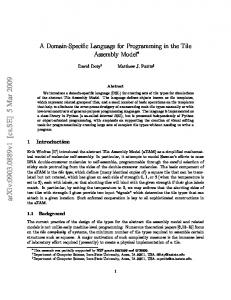
Figure 2.1: Typical elements found in RNA secondary structure. While today the prediction of RNA 3D structure is inaccessible to computational methods, its secondary structure, given by the set of paired bases, can be predicted quite reliably. Figure 2.1 gives examples of typical elements found in RNA secondary structure, called stacking regions (or helices), bulge loops, internal loops, hairpin loops and multiple loops. The first approach to structure prediction was proposed by Nussinov in 1978 and was based on the idea of maximizing the number of base pairs [34]. Today’s algorithms are typically based on energy minimization.
2.2.2
ADP methodology
When designing a dynamic programming algorithm in algebraic style, we need to specify four constituents: • Alphabet: How is the input sequence given? • Search space: What are the elements of the search space and how can they be represented? • Scoring: Given an element of the search space, how do we score it? • Objective: Given a number of scores, which are the ones we are interested in?
19
2.2. ALGEBRAIC DYNAMIC PROGRAMMING BY EXAMPLE
In the following, we will work through these steps for the RNA secondary structure prediction problem. Alphabet The input RNA sequence is a string over A = {a, c, g, u}. A is called the alphabet and A∗ denotes the set of sequences over A of arbitrary length. ε denotes the empty string. In the following, we denote the input sequence with w ∈ A∗ . Search space Given the input sequence w, the search space is the set of all possible secondary structures the sequence w can form. In the ADP terminology, the elements of the search space for a given input sequence are called candidates. Our next task is to decide how to represent such candidates. Two possible ways are shown in Figure 2.2. The first variant is the well-known dot-bracket notation, where pairs of matching parentheses are used to denote pairing bases. The second variant, the tree representation, is the one we use in the algebraic approach. gucaugcaguguca .(.(((...))).) gucaugcaguguca t2 =
(...)((...))..
Split
t1 =
Right
Pair
Split
Nil
’g’
Split
’u’
Right ’g’
Split
Nil
Right ’u’
Right Nil
’g’ ’a’ ’c’
’c’
Pair Split
Right Nil
Split
Right
Pair
’u’
Nil Right
’a’
Split
Pair
’u’ ’g’
Right Nil
Right
’c’
Pair
’a’
Pair
’u’
’u’
Pair
’g’
’g’
Split
’a’
Nil
’c’
’c’
Right ’a’
Right Nil
’u’
’u’ ’g’
Right Nil
Right ’c’
Right Nil
’g’ ’a’
Figure 2.2: Two candidates in the search space for the best secondary structure for the sequence gucaugcaguguca. Such a tree representation of candidates is quite commonly used in RNA structure analysis, but not so in other applications of dynamic programming. To appreciate the scope of the ADP method, it is important to see that such a representation exists for any application of dynamic programming [49]. In our example, the trees are constructed using four different node labels. Each label represents a different situation, which we want to distinguish in the search space and in the eventual scoring of such a candidate. A node labeled pair represents the paring of two bases in the input sequence. The remaining nodes right, split and nil represent unpaired,
20
CHAPTER 2. ALGEBRAIC DYNAMIC PROGRAMMING
branching and empty structures. It is easy to see that each tree is a suitable representation of the corresponding dot-bracket string. Also note that in each of the example trees, the original sequence can be retrieved by collecting the leaves in a counter-clockwise fashion. This is what we call the yield of the tree. The yield function y maps candidate trees back onto their corresponding sequences. The next important concept is the notion of the signature. The signature describes the interface to the scoring functions needed in our algorithm. We can derive the signature for our current example by simply interpreting each of the candidate trees’ node labels as a function declaration: nil : right : pair : split :
A
× Ans
{ε} Ans Ans ×
× × Ans
A A
→ → → →
Ans Ans Ans Ans
The symbol Ans is the abstract result domain. In the following, Σ denotes the signature, TΣ the set of trees over the signature Σ. With the concepts of yield and signature we are now prepared to give a first definition of the search space: Given an input sequence w and a signature Σ, the search space P (w) is the subset of trees from TΣ , whose yield equals w. More formally, P (w) = {t ∈ TΣ |y(t) = w}. This would suffice as a very rough description of the search space. In general, we want to impose more restrictions on it, for example, we want to make sure, that the operator pair is only used in combination with valid base pairs. For this purpose we introduce the notion of tree grammar. Figure 2.3 shows grammar nussinov78, origin of our two example trees. This grammar consists of only one nonterminal, s, and one production with four alternatives, one for each of the four function symbols that label the nodes. Z denotes the axiom of the grammar. The symbols base and empty are terminal symbols, representing an arbitrary base and the empty sequence. The symbol basepairing is a syntactic predicate that guarantees that only valid base pairs can form a pair -node. Z =s
nussinov78 s →
nil
| right
pair
|
| split
with basepairing empty
s
base
base
s
base
s
s
Figure 2.3: Tree grammar nussinov78. Our refined definition of the search space is the following: Given a tree grammar G over Σ and A and a sequence w ∈ A∗ , the language described by G is L(G) = {t|t ∈ TΣ , t can be derived from the axiom via the rules of G}. The search space spawned by w is PG (w) = {t ∈ L(G)|y(t) = w}.
2.2. ALGEBRAIC DYNAMIC PROGRAMMING BY EXAMPLE
21
From the language theoretic viewpoint, PG (w) is the set of all parses of the sequence w for grammar G. The method we use for constructing the search space is called yield parsing. See Section 2.5 for a detailed description of yield parsing. Scoring Given an element of the search space as a tree t ∈ L(G), we need to score this element. In our example we are only interested in counting base pairs, so scoring is very simple: The score of a tree is the number of pair -nodes in t. For the two candidates of Figure 2.2 we obtain scores of 3 (t1 ) and 4 (t2 ). To implement this, we provide definitions for the functions that make up our signature Σ: Ansbpmax nilbpmax (s) rightbpmax (s,b) pairbpmax (a,s,b) splitbpmax (s,s’)
= = = = =
IN 0 s s + 1 s + s’
In mathematics, the interpretation of a signature by a concrete value set and functions operating thereon is called an algebra. Hence, scoring schemes are algebras in ADP. Our first example is the algebra bpmax for maximizing the number of base pairs. The subscript bpmax attached to the function names indicates, that these definitions are interpretations of the function under this algebra. In the following, we will omit these subscripts. The flexibility of the algebraic approach lies in the fact that we don’t have to stop with definition of one algebra. Simply define another algebra and get other results for the same search space. We will introduce a variety of algebras for our second, more elaborate example in Section 2.2.3. Objective The tree grammar describes the search space, the algebra the scoring of solution candidates. Still missing is our optimization objective. For this purpose we add an objective function h to the algebra which chooses one or more elements from a list of candidate scores. An algebra together with an objective function forms an evaluation algebra. Thus algebra bpmax becomes: Ansbpmax
=
IN
bpmax = (nil, right, pair, split, h) where nil(s) right(s,b) pair(a,s,b) split(s,s’) h([]) h([s1 , . . . , sr ])
= = = = = =
0 s s + 1 s + s’ [] [ max si ] 1≤i≤r
A given candidate t can be evaluated in many different algebras; we use the notation E(t) to indicate the value obtained from t under evaluation with algebra E.
22
CHAPTER 2. ALGEBRAIC DYNAMIC PROGRAMMING
Given that yield parsing constructs the search space for a given input, all that is left to do is to evaluate the candidates in a given algebra, and make our choice via the objective function h. For example, candidates t1 and t2 of Figure 2.2 are evaluated by algebra bpmax in the following way: = =
h(bpmax(t1 ), bpmax(t2 )) [max(3, 4)] [4]
Definition 1 (Algebraic dynamic programming) • An ADP problem is specified by a signature Σ over A, a tree grammar G over Σ, and a Σ-evaluation algebra E with objective function h. • An ADP problem instance is posed by a string w ∈ A∗ . Its search space is the set of all its parses, PG (w). • Solving an ADP problem is computing h{E(t) | t ∈ PG (w)} in polynomial time and space with respect to |w|. In general, Bellman’s Principle of Optimality [2] must be satisfied in order to achieve polynomial efficiency. Definition 2 (ADP formulation of Bellman’s Principle) An evaluation algebra satisfies Bellman’s Principle, if for each k-ary function f in Σ and all answer lists z 1 , . . . , zk , the objective function h satisfies h([f (x1 , . . . , xk ) | x1 ← z1 , . . . , xk ← zk ]) = h([f (x1 , . . . , xk ) | x1 ← h(z1 ), . . . , xk ← h(zk )]) as well as h( z ++ z 0 ) = h( h(z) ++ h(z 0 ) ) where ++ denotes list concatenation, and ← denotes list membership. Bellman’s Principle, when satisfied, allows the following implementation: As the trees that constitute the search space are constructed by the yield parser in a bottom up fashion, rather than building them explicitly as elements of TΣ , for each function symbol f the evaluation function fE is called. Thus, the yield parser computes not trees, but their evaluations. To reduce their number (and thus to avoid exponential explosion) the objective function may be applied at an intermediate step where a list of alternative answers has been computed. Due to Bellman’s Principle, the recursive intermediate applications of the objective function do not affect the final result. As an example, consider the following two candidates (represented as terms) in the search space for sequence aucg:
2.2. ALGEBRAIC DYNAMIC PROGRAMMING BY EXAMPLE t3 = Split (Pair ’a’ Nil (Right (Right t4 = Split (Pair ’a’ Nil (Pair ’c’ Nil
23
’u’) Nil ’c’) ’g’) ’u’) ’g’)
Since algebra bpmax satisfies Bellman’s Principle, we can apply the objective function h at intermediate steps inside the evaluation of candidates t3 and t4 : =
=
= = =
h(bpmax(t3 ), bpmax(t4 )) h(Split (Pair ’a’ Nil ’u’) (Right (Right Nil ’c’) ’g’), Split (Pair ’a’ Nil ’u’) (Pair ’c’ Nil ’g’)) h(Split (h(Pair ’a’ Nil ’u’, Pair ’a’ Nil ’u’)) (h(Right (Right Nil ’c’) ’g’, Pair ’c’ Nil ’g’))) [max(max(1, 1) + max(0, 1))] [max(1 + 1)] [2]
Given grammar and signature, the traditional dynamic programming recurrences can be derived mechanically to implement the yield parser. In the sequel, we shall use the name of a grammar as the name of the function that solves the dynamic programming problem at hand. Naturally, it takes two arguments, the evaluation algebra and the input sequence.
2.2.3
In-depth search space analysis
Note that the case analysis in the Nussinov algorithm is redundant – even the sequence ‘aa’ is assigned the two trees Right (Right Nil ’a’) ’a’ and Split (Right Nil ’a’) (Right Nil ’a’), which actually denote the same structure. In order to study also suboptimal solutions, a non-redundant algorithm was presented in [57]. Figure 2.4 shows the grammar wuchty98. Here the signature has 8 function symbols, each one modeling a particular structure element, plus the list constructors (nil, ul, cons) to collect sequences of components in a unique way. Nonterminal symbol strong is used to capture structures without isolated (unstacked) base pairs, as those are known to be energetically unstable. Purging them from the search space decreases the number of candidates considerably. This grammar, because of its non-redundancy, can also be used to study combinatorics, such as the expected number of feasible structures of a sequence of length n. This algorithm, as implemented in RNAsubopt [57], is widely used for structure prediction via energy minimization. The thermodynamic model is too elaborate to be presented here,
24
CHAPTER 2. ALGEBRAIC DYNAMIC PROGRAMMING
Z = struct
wuchty98 struct →
str
str
|
comps
comps →
ul
nil
singlestrand
empty
cons
ul
|
comps
block
block → strong |
str
|
region
block
strong
ss
singlestrand →
cons
|
block
bl
ul
region
singlestrand strong →
sr
sr
|
) with basepairing
( base
strong
weak →
base
hl
( base
weak
base
sr
|
region3
base
base
cons
block
base strong
base strong
br
|
base region
sr
|
base
base
comps
sr
|
bl
base region
ml
base
region
il strong
base
) with basepairing
region
region3 → region with minsize 3
Figure 2.4: Tree grammar wuchty98.
25
2.2. ALGEBRAIC DYNAMIC PROGRAMMING BY EXAMPLE
Ansenum
enum
= (str, ..., h) str(s) ss((i,j)) hl(a,(i,j),b) sr(a,s,b) bl((i,j),s) br(s,(i,j)) il((i,j),s,(i’,j’)) ml(a,s,b) nil((i,j)) cons(s,s’) ul(s) h([s1 , . . . , sr ]) Ansbpmax
=
Anspretty
TΣ
where = Str s = Ss (i,j) = Hl a (i,j) b = Sr a s b = Bl (i,j) s = Br s (i,j) = Il (i,j) s (i’,j’) = Ml a s b = Nil (i,j) = Cons s s’ = Ul s = [s1 , . . . , sr ] =
IN
bpmax
= (str, ..., h) where str(s) = s ss((i,j)) = 0 hl(a,(i,j),b) = 1 sr(a,s,b) = s + 1 bl((i,j),s) = s br(s,(i,j)) = s il((i,j),s,(i’,j’)) = s ml(a,s,b) = s + 1 nil((i,j)) = 0 cons(s,s’) = s + s’ ul(s) = s h([]) = [] h([s1 , . . . , sr ]) = [ max si ] 1≤i≤r
= (str, ..., h) str(s) = ss((i,j)) = hl(a,(i,j),b) = sr(a,s,b) = bl((i,j),s) = br(s,(i,j)) = il((i,j),s,(i’,j’)) = ml(a,s,b) nil((i,j)) cons(s,s’) ul(s) h([s1 , . . . , sr ]) Anscount
dot-bracket strings
=
pretty
= = = = =
where s dots(j-i) "("++dots(j-i)++")" "("++s++")" dots(j-i)++s s++dots(j-i) dots(j-i)++s++ dots(j’-i’) "("++s++")" "" s++s’ s [s1 , . . . , sr ] =
IN
count
= (str, ..., h) where str(s) = s ss((i,j)) = 1 hl(a,(i,j),b) = 1 sr(a,s,b) = s bl((i,j),s) = s br(s,(i,j)) = s il((i,j),s,(i’,j’)) = s ml(a,s,b) = s nil((i,j)) = 1 cons(s,s’) = s * s’ ul(s) = s h([]) = [] h([s1 , . . . , sr ]) = [s1 + · · · + sr ]
Figure 2.5: Four evaluation algebras for grammar wuchty98. Arguments a and b denote bases, (i,j) represents the input subword wi+1 . . . wj , and s denotes answer values. Function dots(r) in algebra pretty yields a string of r dots (’.’) .
26
CHAPTER 2. ALGEBRAIC DYNAMIC PROGRAMMING
and we will stick with base pair maximization as our optimization objective for the sake of this presentation. Figure 2.5 shows four evaluation algebras that we will use with grammar wuchty98. We illustrate their use via the following examples, where g(a,w) denotes the application of grammar g and algebra a to input w. Table 2.1 summarizes all results for an example sequence. Application wuchty98(enum,w)
wuchty98(pretty,w) wuchty98(bpmax,w) wuchty98(count,w) nussinov78(count,w)
Result [Str (Ul (Bl (0,1) (Sr ’g’ (Hl ’g’ (3,10) ’c’) ’u’))), Str (Ul (Bl (0,2) (Sr ’g’ (Hl ’g’ (4,10) ’c’) ’u’))), Str (Cons (Bl (0,1) (Sr ’g’ (Hl ’g’ (3,7) ’c’) ’c’)) (Ul (Ss (9,12)))), Str (Cons (Bl (0,2) (Sr ’g’ (Hl ’g’ (4,7) ’c’) ’c’)) (Ul (Ss (9,12)))), Str (Ul (Ss (0,12)))] [".((.......))", "..((......))", ".((....))...", "..((...))...", "............"] [2] [5] [9649270]
Table 2.1: Applications of grammars wuchty98 and nussinov78 with different individual algebras on input w = cgggauaccacu. wuchty98(enum,w): The enumeration algebra enum yields unevaluated terms. By convention, function symbols are capitalized in the output. Since the objective function is identity, this call enumerates all candidates in the search space spawned by w. This is mainly useful in program debugging, as it allows us to inspect the search space actually traversed by our program. wuchty98(pretty,w): The pretty-printing algebra pretty yields a dot-bracket string representation of the same structures as the above. wuchty98(bpmax,w): The base pair maximization algebra is bpmax, such that this call yields the maximal number of base pairs that a structure for w can attain. Here the objective function is maximization, and it can be easily shown to satisfy Bellman’s Principle. Similarly for grammar nussinov78. wuchty98(count,w): The counting algebra count has as its objective function summation, and Ecount (t) = 1 for all candidates t. Hence, summing over all candidate scores gives the number of candidates. However, the evaluation functions are carefully written such that they satisfy Bellman’s Principle. Thus, [length(wuchty98(enum,w))] == wuchty98(count,w)1 , where the right-hand side is polynomial to compute, while the left-hand side typically is exponential due to the large number of answers returned by wuchty98(enum,w). nussinov78(count,w): This computes (using an analogous version of the counting algebra not shown here) the number of structures considered by the Nussinov algorithm, which, in 1 Technically,
the result of wuchty98(count,w) is a singleton list, hence the [. . . ].
2.3. THE PRODUCT OPERATION ON EVALUATION ALGEBRAS
27
contrast to the above, is much larger than the size of the search space. These examples show analyses achieved by individual algebras. We now turn to what can be done by their combination.
2.3
The product operation on evaluation algebras
In this section we first introduce and discuss our definition of the product operation. From there, we proceed with a series of examples demonstrating its usage.
2.3.1
Definition
We define the product operation as follows: Definition 3 (Product operation on evaluation algebras) Let M and N be evaluation algebras over Σ. Their product M ***N is an evaluation algebra over Σ and has the functions fM ***N ((m1 , n1 )...(mk , nk )) = (fM (m1 , ..., mk ), fN (n1 , ..., nk )) for each f in Σ,
and the objective function hM ***N ([(m1 , n1 )...(mk , nk )]) = [(l, r)| l ∈ L, r ← hN ([r0 |(l0 , r0 ) ← [(m1 , n1 )...(mk , nk )], l0 = l])], where L = hM ([m1 , ..., mk ]).
We illustrate this mechanism on the application of the product operation on algebras bpmax and count: Ansbpmax
=
*** count
bpmax *** count
IN × IN
= (str, ..., h) where str((m,n)) = (m,n) ss((i,j)) = (0,1) hl(a,(i,j),b) = (1,1) sr(a,(m,n),b) = (m + 1,n) bl((i,j),(m,n)) = (m,n) br((m,n),(i,j)) = (m,n) il((i,j),(m,n),(i’,j’)) = (m,n) ml(a,(m,n),b) = (m + 1,n) nil((i,j)) = (0,1) cons((m,n),(m’,n’)) = (m + m’, n * n’) ul((m,n)) = (m,n) h([(m1 , n1 )...(mk , nk )]) = [(l, r)|l P∈ 0L, 0 0 r ← [ [r |(l , r ) ← [(m1 , n1 )...(mk , nk )], l0 = l]]], where L = [ max mi ] 1≤i≤k
28
CHAPTER 2. ALGEBRAIC DYNAMIC PROGRAMMING
Here, each function calculates a pair of two result values. The first is the result of algebra bpmax, the second is the result of algebra count. The interesting part is the objective function h. It receives the list of pairs as input, with each pair consisting of the candidate’s scores for the first and for the second algebra. In the first step the objective function of algebra bpmax (max) is applied to the list of the first pair elements. The result is stored in L. Then, for each element2 of L, a new intermediate list is constructed that consists of all corresponding right pair elements of the input list. This intermediate list is then applied to the objective function of the second algebra (here: summation). Finally, the result of h is constructed by combination of all elements from L with their corresponding result for the second algebra stored in r. This computes the optimal number of base pairs, together with the number of candidate structures that achieve it. Above, ∈ denotes set membership and hence ignores duplicates. In contrast, ← denotes list membership and respects duplicates. Implementing set membership may require some extra filtering effort, but when the objective function hM , which computes L, does not produce duplicates anyway, it comes for free. One should not rely on intuition alone for understanding what M ***N actually computes. For any tree grammar G and product algebra M ***N , their combined meaning is well defined by Definition 1, and the view that a complete list of all candidates is determined first, with hM ***N applied only once in the end, is very helpful for understanding. But does G(M ***N, w) actually do what it means? The implementation works correctly if and only if Bellman’s Principle is satisfied by M ***N , which is not implied when it holds for M and N individually! Hence, use of product algebras is subject to the following Proof obligation: Prove that M ***N satisfies Bellman’s Principle (Definition 2). Alas, we have traded the need of writing and debugging code for a proof obligation. Fortunately, there is a theorem that covers many important cases3 : Theorem 1 (1) For any algebras M and N , and answer list x, (idM ∗ ∗ ∗ idN )(x) is a permutation of x. (2) If hM and hN minimize with respect to some order relations ≤M and ≤N , then hM ***N minimizes with respect to the lexicographic ordering (≤M , ≤N ). Proof. (1) According to Definition 3, the elements of x are merely re-grouped according to their first component. For this to hold, it is essential that L is treated as a set. (2) follows directly from Definition 3. � 2 In
this example, L holds only one element, namely the maximum base pair score of the input list. [49], the theorem erroneously contains also the following statement: If both M and N minimize as above and both satisfy Bellman’s Principle, then so does M ***N . This property would be nice to have, but there exist counterexamples where it does not hold. 3 In
2.3. THE PRODUCT OPERATION ON EVALUATION ALGEBRAS
29
In the above proof, strict monotonicity is required only if we ask for multiple optimal, or for the k best solutions rather than a single, optimal one [33]. Theorem 1 (1) justifies our peculiar treatment of the list L as a set. It states that no elements of the search space are lost or get duplicated by the combination of two algebras. Theorem 1 (2,3) say that *** behaves as expected in the case of optimizing evaluation algebras. This is very useful, but not too surprising. A surprising variety of applications arises when *** is used with algebras that do not do optimization, like enum, count, and pretty. The proof obligation is met for all the applications studied below. A case where the proof fails is, for example, wuchty98(count***count,w), which consequently delivers no meaningful result.
2.3.2
Implementing the product operation
The algebraic style of dynamic programming can be practiced within any decent programming language. It is mainly a discipline of structuring our dynamic programming algorithms, the perfect separation of problem decomposition and scoring being the main achievement. When using the ASCII notation for tree grammars proposed in [17], the grammars can be compiled into executable code. Otherwise, one has to derive the explicit recurrences and implement the corresponding yield parser. Care must be taken to keep the implementation of the recurrences independent of the result data type, such that they can be run with different algebras, including arbitrary products. All this given, the extra effort for using product algebras is small. It amounts to implementing the defining equations for the functions of M ***N generically, i.e. for arbitrary evaluation algebras M and N over the common signature Σ. In a language which supports functions embedded in data structures, this is one line per evaluation function, witnessed by our implementation in Haskell (available for download). In other languages, abstract classes (Java) or templates (C++) can be used. It is essential to provide a generic product implementation. Otherwise, each new algebra combination must be hand-coded, which is not difficult to do, but tedious and error-prone, and hence necessitates debugging. A generic product, once tested, guarantees absence of errors for all combinations.
2.3.3
Efficiency discussion
Before we turn to the uses of ***, a word on computational efficiency seems appropriate. Our approach requires to structure programs in a certain way. This induces a small (constant factor) overhead in space and time. For example, we must generically return a list of results, even with analyses that return only a single optimal value. Normally, each evaluation function is in O(1), and when h returns a single answer, asymptotic efficiency is solely determined by the tree grammar [17]. This asymptotic efficiency remains unaffected when we use a product algebra. Each table entry now holds a pair of answers, each of size O(1).
30
CHAPTER 2. ALGEBRAIC DYNAMIC PROGRAMMING
Things change when we employ objective functions that produce multiple results, as the size of the desired output can become exponential in n, and then it dominates the overall computational effort. For example, the optimal base pair score may be associated with a large number of co-optimal candidates, especially when the grammar is ambiguous. Thus, if using *** makes our programs slower (asymptotically), it is not because of an intrinsic effect of the product operation, but because we decide to do more costly analyses by looking deeper into the search space. The only exception to this rule is the situation where objective function hM produces duplicate values, which must be filtered out, as described with Definition 3. In this case, a non-constant factor proportional to the length of answer lists is incurred. The concrete effect of using product algebras on CPU time and space is difficult to measure, as the product algebra runs a more sophisticated analysis than either single one. For an estimation, we measure the (otherwise meaningless) use of the same algebra twice. We compute wuchty98(bpmax,w) and compare to wuchty98(bpmax***bpmax,w). The outcome is shown in Table 2.2. For input lengths from 200 to 1600 bases, the product algebra uses 9.57% to 21.34% more space and is 18.97% to 29.46% slower than the single algebra. time (sec) space (MB) time (sec) space (MB) time (sec) space (MB) time (sec) space (MB)
|w| 200 200 400 400 800 800 1600 1600
wuchty98(bpmax,w) 0.58 1.88 4.65 4.60 52.04 15.61 590.72 59.85
wuchty98(bpmax***bpmax,w) 0.69 2.06 6.02 5.37 65.54 18.77 725.03 72.62
% + 18.97 + 9.57 + 29.46 + 16.74 + 25.94 + 20.24 + 22.74 + 21.34
Table 2.2: Measuring time and space requirements of the product operation. All results are for a C implementation of wuchty98, running on a 900 MHz Ultra Sparc 3 CPU under Sun Solaris 10. The space requirements were measured using a simple wrapper function for malloc, that counts the number of allocated bytes. Times were measured with gnu time.
2.3.4
Applications of product algebras
We now turn to applications of product algebras. Table 2.3 summarizes all results of the analyses discussed in the sequel, for a fixed example RNA sequence. Application 1: Backtracing and co-optimal solutions Often, we want not only the optimal answer value, but also a candidate which achieves the optimum. We may ask if there are several optimal candidates. If so, we may want to see them all, maybe even including some near-optimal candidates. The traditional technique
2.3. THE PRODUCT OPERATION ON EVALUATION ALGEBRAS
Application wuchty98(bpmax***count,w) wuchty98(bpmax***pretty,w) wuchty98(bpmax***enum,w)
wuchty98(bpmax***(enum***pretty),w)
wuchty98(shape***count,w) wuchty98(bpmax(5)***shape,w) wuchty98(bpmax(5)***(shape***count),w) wuchty98(shape***bpmax,w) wuchty98(bpmax***pretty’,w) wuchty98(pretty***count,w)
31
Result [(2,4)] [(2,".((.......))"), (2,"..((......))"), (2,".((....))..."), (2,"..((...))...")] [(2,Str (Ul (Bl (0,1) (Sr ’g’ (Hl ’g’ (3,10) ’c’) ’u’)))),(2,Str (Ul (Bl (0,2) (Sr ’g’ (Hl ’g’ (4,10) ’c’) ’u’)))),(2,Str (Cons (Bl (0,1) (Sr ’g’ (Hl ’g’ (3,7) ’c’) ’c’)) (Ul (Ss (9,12))))),(2,Str (Cons (Bl (0,2) (Sr ’g’ (Hl ’g’ (4,7) ’c’) ’c’)) (Ul (Ss (9,12)))))] [(2,(Str (Ul (Bl (0,1) (Sr ’g’ (Hl ’g’ (3,10) ’c’) ’u’))), ".((.......))")), (2,(Str (Ul (Bl (0,2) (Sr ’g’ (Hl ’g’ (4,10) ’c’) ’u’))), "..((......))")), (2,(Str (Cons (Bl (0,1) (Sr ’g’ (Hl ’g’ (3,7) ’c’) ’c’)) (Ul (Ss (9,12)))), ".((....))...")), (2,(Str (Cons (Bl (0,2) (Sr ’g’ (Hl ’g’ (4,7) ’c’) ’c’)) (Ul (Ss (9,12)))), "..((...))..."))] [(" [ ]",2), (" [ ] ",2), (" ",1)] [(2," [ ]"), (2," [ ] "), (0," ")] [(2,(" [ ]",2)), (2,(" [ ] ",2)), (0,(" ",1))] [(" [ ]",2), (" [ ] ",2), (" ",0)] [(2,".((....))...")] [(".((.......))",1), ("..((......))",1), (".((....))...",1), ("..((...))...",1), ("............",1)]
Table 2.3: Example applications of product algebras with grammar wuchty98 on input w = cgggauaccacu.
32
CHAPTER 2. ALGEBRAIC DYNAMIC PROGRAMMING
is to store a table of intermediate answers and backtrace through the optimizing decisions made [21]. This backtracing can become quite intricate to program if we ask for more than one candidate. We can answer these questions without additional programming efforts using products: wuchty98(bpmax***count,w) computes the optimal number of base pairs, together with the number of candidate structures that achieve it. wuchty98(bpmax***enum,w) computes the optimal number of base pairs, together with all structures for w that achieve this maximum, in their representation as terms from TΣ . wuchty98(bpmax***pretty,w) does the same as the previous call, producing the string representation of structures. wuchty98(bpmax***(enum***pretty),w) does both of the above. To verify all these statements, apply Definition 3, or visit the ADP web site and run your own examples. It is a nontrivial consequence of Definition 3 that the above product algebras in fact give all co-optimal solutions. Should only a single one be desired, we would use enum or pretty with a modified objective function h that retains only one element. Note that our substitution of backtracing by a “forward” computation does not affect asymptotic runtime efficiency. With bpmax***enum, for example, the algebra stores in each table entry the optimal base pair count, together with the top node of the optimal candidate(s) and pointers to its immediate substructures, which reside in other table entries. Hence, even if there should be an exponential number of co-optimal answers, they are represented in polynomial space, because subtrees are shared. Should the user decide to have them all printed, exponential effort is incurred, just as with a backtracing implementation.
Application 2: Holistic search space analysis Abstract shapes were recently proposed in [20] as a means to obtain a holistic view of an RNA molecule’s folding space, avoiding the explicit enumeration of a large number of structures. Bypassing all relevant mathematics, let us just say that an RNA shape is an object that captures structural features, like the nesting pattern of stacking regions, but not their size. We visualize shapes by strings alike dot-bracket notation, such as [ [ ]], where denotes an unpaired region and [ together with the matching ] denotes a complete helix of arbitrary length. This is achieved by the following shape algebra:4
4 The
function shMerge appends two strings and merges adjacent characters for unpaired regions ( ). The function nub eliminates duplicates from its input list.
2.3. THE PRODUCT OPERATION ON EVALUATION ALGEBRAS
Ansshape
=
33
shape strings
shape = (str, ..., h) where str(s) ss((i,j)) hl(a,(i,j),b) sr(a,s,b) bl((i,j),s) br(s,(i,j)) il((i,j),s,(i’,j’)) ml(a,s,b) nil((i,j)) cons(s,s’) ul(s) h([s1 , . . . , sr ])
= = = = = = = = = = = =
s "" "[ ]" s " "++s s++" " " "++s++" " "["++s++"]" "" shMerge(s,s’) s nub[s1 , . . . , sr ]
Together with a creative use of ***, the shape algebra allows us to analyze the number of possible shapes, the size of their membership, and the (near-) optimality of members, and so on. Let bpmax(k) be bpmax with an objective function that retains the best k answers (without duplicates). wuchty98(shape***count,w) computes all the shapes in the search space spawned by w, and the number of structures that map onto each shape. wuchty98(bpmax(k)***shape,w) computes the best k base pair scores, together with their candidates’ shapes. wuchty98(bpmax(k)***(shape***count),w) computes base pairs and shapes as above, plus the number of structures that achieve this number of base pairs in the given shape. wuchty98(shape***bpmax,w) computes for each shape the maximum number of base pairs among all structures of this shape.
Application 3: Optimization under lexicographic orderings Theorem 1 is useful in practice as one can test different objectives independently and then combine them in one operation. A simple case of using two orderings would be the following: Assume we have a case with a large number of co-optimal solutions. Let pretty’ be pretty with h = min. wuchty98(bpmax***pretty’,w) computes among several optimal structures the one which comes alphabetically first according to its string representation.5 5 Of
course, there are more meaningful uses of a primary and a secondary optimization objective. For lack of space, we refrain from introducing another optimizing algebra here.
34
CHAPTER 2. ALGEBRAIC DYNAMIC PROGRAMMING
Application 4: Testing ambiguity Dynamic programming algorithms can often be written in a simpler way if we do not care whether the same solution is considered many times during the optimization. This does not affect the overall optimum. A dynamic programming algorithm is then called redundant or ambiguous. In such a case, the computation of a list of near-optimal solutions is cumbersome, as it contains duplicates whose number often has an exponential growth pattern. Also, search space statistics become problematic – for example, the counting algebra speaks about the algorithm rather than the problem space, as it counts evaluated, but not necessarily distinct solutions. Tree grammars with a suitable probabilistic evaluation algebra implement stochastic context free grammars (SCFGs) [8]. The frequently used statistical scoring schemes, when trying to find the answer of maximal probability (the Viterbi algorithm, cf. [8]), are fooled by the presence of redundant solutions. In principle, it is clear how to control ambiguity [14]. One needs to show unambiguity of the tree grammar 6 in the language theoretic sense, and the existence of an injective mapping from TΣ to a canonical model of the search space. However, the proofs involved are not trivial. Rather, one would like to implement a check for ambiguity that is applicable for any given tree grammar, but this may be difficult or even impossible, as the problem is closely related to ambiguity of context free languages, which is known to be formally undecidable. Recently, Dowell and Eddy showed that ambiguity really matters in practice for SCFG design, and they suggest a procedure for ambiguity testing [7]. This test uses a combination of Viterbi and Inside algorithms to check whether the (putatively optimal) candidate returned by Viterbi has an alternative derivation. A more complete test is the following, and due to the use of ***, it requires no implementation effort: The required homomorphism from the search space to the canonical model may be coded as another evaluation algebra. In fact, if we choose the dot-bracket string representation as the canonical model, algebra pretty does exactly this. We can test for ambiguity by testing injectivity of pretty – by calling wuchty98(pretty***count,w) on a number of inputs w. If any count larger than 1 shows up in the results, we have proved ambiguity. This test is strictly stronger than the one by Dowell and Eddy, which detects ambiguity only if it occurs with the (sampled) “near-optimal” predictions. This and other test methods are studied in detail in [41]. Limitations of the product operation The above applications demonstrate the considerable versatility of the algebra product. In particular, since a product algebra is an algebra itself, we can work with algebra triples, quadruples, and so on. All of these will be combined in the same fashion, and here we reach the limits of the product operation. 6 Not
the associated string grammar – it is always ambiguous, else we would not have an optimization problem.
2.4. CONCLUSION
35
The given definition of *** is not the only way needed to combine two algebras. In abstract shape analysis [20], we use three algebras mfe (computing minimal free energy), shape and pretty. A shape representative structure is the structure of minimal free energy within the shape. Similarly to the above, wuchty98(shape***(mfe***pretty),w) computes the representatives of all shapes. However, computing only the k best shape representatives requires minimization within and across shapes, which neither mfe***shape nor shape***mfe can achieve. Hence, a hand-coded combination of the three algebras is necessary for this particular analysis.
2.4
Conclusion
We hope to have demonstrated that the evaluation algebra product as introduced here adds a significant amount of flexibility to dynamic programming. We have shown how ten meaningful analyses with quite diverse objectives can be obtained by using different products of a few simple algebras. The techniques we have shown here pertain not just to RNA folding problems, but to all dynamic programming algorithms that can be formulated in the algebraic style. The benefits from using a particular coding discipline do not come for free. There is some learning effort required to adapt to a systematic approach and to abandon traditional coding habits. After that, the discipline pays back by making programmers more productive. Yet, the pay-off is hard to quantify. We therefore conclude with a subjective summary of our experience as bioinformatics toolsmiths. After training a generation of students on the concepts presented here, we have enjoyed a boost in programming productivity. Four bioinformatics tools have been developed using this approach – pknotsRG [39], RNAshapes [20], RNAhybrid [42] and RNAcast [40]. The “largest” example is the pseudoknot folding grammar, which uses 47 nonterminal symbols and a 140-fold case distinction. The techniques described here have helped to master such complexity in several ways: • The abstract formulation of dynamic programming recurrences in the form of grammars makes it easy to communicate and refine algorithmic ideas. • Writing non-ambiguous grammars for optimization problems allows us to use the same algorithm for mathematical analysis of the search space. • Ambiguity checking ensures us that such analyses are correct, that probabilistic analyses are not fooled by redundant recurrences, and that near-optimal solutions when reported do not contain duplicates. • enum algebras allow for algorithm introspection – we can obtain a protocol of all solution candidates the program has seen, a quite effective program validation aid.
36
CHAPTER 2. ALGEBRAIC DYNAMIC PROGRAMMING • Using pretty and enum algebras in products frees us from the tedious programming of backtracing routines. • The use of the product operation allows us to create new analyses essentially with three key strokes – and a proof obligation that must be met.
This has created a good testbed for the development of new algorithmic ideas, which can immediately be put to practice.
2.5
Algebraic Dynamic Programming as a domain specific language This section is taken from [17].
ADP has been designed as a domain specific language embedded in Haskell [37]. An algorithm written in ADP notation can be directly executed as a Haskell program. Of course, this requires that the functions of the evaluation algebra are coded in Haskell. A smooth embedding is achieved by adapting the technique of parser combinators [26], which literally turn the grammar into a parser. Hutton’s technique applies to context free grammars and string parsing. We need to introduce suitable combinator definitions for yield parsing, and add tabulation. Generally, a parser is a function that, given a subword of the input, returns a list of all its parses: > type Subword = (Int,Int) > type Parser b = Subword -> [b]
2.5.1
Lexical parsers
The lexical parser achar recognizes any single character. Parser astring recognizes a (possibly empty) subword and parser astringp a nonempty subword. Specific characters or strings are recognized by char and string. Parser empty recognizes the empty subword and parser loc provides the current location in the input sequence. > empty > empty
:: Parser () (i,j) = [() | i == j]
> achar > achar
:: Parser Char (i,j) = [z!j | i+1 == j]
> astring :: Parser Subword > astring (i,j) = [(i,j) | i astringp :: Parser Subword > astringp (i,j) = [(i,j) | i < j] > char :: Char -> Parser Char > char c (i,j) = [c | i+1 == j, z!j == c] > string :: String -> Parser Subword > string s (i,j) = [(i,j)| and [z!(i+k) == s!!(k-1) | k loc > loc
(i,j)
:: Parser Int = [i | i == j]
The parsers base and region used in Section 2.2.3 are synonyms for the parsers achar and astring.
2.5.2
Nonterminal parsers
The nonterminal symbols in the grammar are interpreted as parsers, with the productions serving as their mutually recursive definitions. Each righthand side is an expression that combines parsers using the parser combinators.
2.5.3
Parser combinators
The operators introduced in the ADP notation are now defined as parser combinators: ||| concatenates result lists of alternative parses, (|||) :: Parser b -> Parser b -> Parser b > (|||) r q (i,j) = r (i,j) ++ q (i,j) > infix 8 ( c) -> Parser b -> Parser c > (~~~) r q (i,j) = [f y | k ([b] -> [b]) -> Parser b > (...) r h (i,j) = h (r (i,j))
38
CHAPTER 2. ALGEBRAIC DYNAMIC PROGRAMMING
Note that the operator priorities are defined such that an expression f with q c (i,j) = if c (i,j) then q (i,j) else [] > axiom > axiom ax
:: Parser b -> [b] = ax (0,l)
When a parser is called with the enumeration algebra – i.e. the functions applied are actually tree constructors, and the objective function is the identity function – then it behaves like a proper yield parser and generates a list of trees according to Section 2.2.2. However, called with some other evaluation algebra, it computes any desired type of answer.
2.5.4
Tabulation
Adding tabulation is merely a change of data type, replacing a recursive function by a recursively defined table. Now we need a general scheme for this purpose: The function table records the results of a parser p for all subwords of an input of size n, and returns as its result a function that does lookup in this table. Note the essential invariance (table n f)!(i,j) = f(i,j). Therefore, table n p is a tabulated parser, that can be used in place of parser p. In contrast to the latter, it does not compute the results for the same subword (i,j) repeatedly – here we enjoy the blessings of lazy evaluation and avoid exponential explosion. The keyword tabulated is now defined as table bound to the global variable l, the length of the input. > table :: Int -> Parser b -> Parser b > table n p = (!) (array ((0,0),(n,n)) > [((i,j), p (i,j)) | i (~~) (l,u) (l’,u’) r q (i,j) > = [x y | k x (nil,left,right,pair,split,h) = alg > > > > > >
s = tabulated ( nil answer, > alphabet -> answer -> answer, > answer -> alphabet -> answer, > alphabet -> answer -> alphabet -> answer, > [answer] -> [answer] > ) Enumeration algebra: > enum :: Algebra Char Alignment > enum = (nil, d, i, r, h) where > nil = Nil > d = D > i = I > r = R > h = id Counting algebra: > count :: Algebra Char Int > count = (nil, d, i, r, h) where > nil a = 1 > d a b = b > i a b = a > r a b c = b > h [] = [] > h xs = [sum xs] Algebra product operation: > (***) :: Eq answer1 => > (Algebra Char answer1) -> > (Algebra Char answer2) -> > Algebra Char (answer1,answer2) > infix *** > alg1 *** alg2 = (nil, d, i, r, h) where > (nil1, d1, i1, r1, h1) = alg1 > (nil2, d2, i2, r2, h2) = alg2 > > nil a = (nil1 a, nil2 a) > d a (b1,b2) = (d1 a b1, d2 a b2) > i (a1,a2) b = (i1 a1 b, i2 a2 b) > r a (b1,b2) c = (r1 a b1 c, r2 a b2 c) > > h xs = [(x1,x2)| x1 > alignment = > > > >
= axiom alignment where r, h) = alg tabulated( nil