Complementary Matching Pursuit Algorithms for Sparse. Approximation. Gagan Rath and Christine Guillemot. IRISA-INRIA, Campus de Beaulieu.
Complementary Matching Pursuit Algorithms for Sparse Approximation Gagan Rath and Christine Guillemot IRISA-INRIA, Campus de Beaulieu 35042 Rennes, France phone: +33.2.99.84.75.26 fax: +33.2.99.84.71.71 e-mail: {grath}{cguillem}@irisa.fr April 25, 2008
Abstract Sparse coding in a redundant basis is of considerable interest in many areas of signal processing. The problem generally involves solving an under-determined system of equations under a sparsity constraint. Except for the exhaustive combinatorial approach, there is no known method to find the exact solution under general conditions on the dictionary. Among the various algorithms that find approximate solutions, pursuit algorithms are the most well-known. In this paper, we introduce the concept of a complementary matching pursuit (CMP). The algorithm is similar to the classical matching pursuit (MP), but performs the complementary action. Instead of selecting one atom to be included in the sparse approximation, it selects (N −1) atoms to be excluded from the approximation at each iteration. Though these two actions seem apparently the same, they are actually performed in two different spaces. On a conceptual level, the MP searches for ’the solution vector among sparse vectors’ whereas the CMP searches for ’the sparse vector among the solution vectors’. We assume that the observations can be expressed as pure linear sums of atoms without any additive noise. As a consequence of the complementary action, the CMP does not minimize the residual error at each iteration, however it may converge faster yielding sparser solution vectors than the MP. We show that when the dictionary is a tight frame, the CMP is equivalent to the MP. We also present the orthogonal extensions of the CMP and show that they perform the complementary actions to those of their classical matching pursuit counterparts.
Keywords — Sparse approximation, Atomic decomposition, Matching pursuit, Basis pursuit, Projection
EDICS: SPC-CODC: Signal representation, coding and compression
1
1
Introduction
Sparse coding in a redundant basis has attracted considerable interest recently because of its application in many areas of signal processing such as compression, denoising, time-frequency analysis, indexing, compressed sensing, audio source separation, etc. The basic problem is to represent a given signal as a linear combination of the fewest signals from a redundant signal set either exactly or with some error less than a specified threhold. Consider a set of N signal vectors arranged as the columns of a matrix A. Each vector has dimension K where K < N . Using the terminology in sparse approximation theory, we will refer to these vectors as atoms and to A as the dictionary matrix. We will assume that the atoms are normalized, i.e., they have unit magnitudes. Given a signal b, the problem is to identify the fewest atoms whose linear sum will approximate b. Mathematically this can be formulated as solving the following system of linear equations: Ax = b,
(1)
such that x has the minimum number of non-zero elements. The sparse approximation problem is thus posed as min{kxk0 : Ax = b},
(2)
where the l0 norm denotes the number of non-zero elements. The sparse coding problem that allows some approximation error is posed as: min{kxk0 : kAx − bk2 ≤ δ},
(3)
for some δ > 0. Here k.k2 denotes the l2 norm. These two problems are NP-hard [1, 2]. Except for the exhaustive combinatorial approach, there is no known method to find the exact solution under general conditions on the dictionary matrix A. Among the various algorithms that find approximate solutions, pursuit algorithms are the most well-known. The matching pursuit (MP) [3] and the orthogonal matching pursuit (OMP) [4, 5] are the simplest and the least complex. The basis pursuit (BP) relaxes the l0 norm condition by the l1 norm and solves the problem through linear programming [6]. It is generally believed that BP algorithms can produce more accurate solutions than the matching pursuit algorithms, but they require higher computational effort. In this paper, we introduce the concept of a complementary matching pursuit (CMP). The algorithm is similar to the classical MP, but performs the complementary action. Instead of selecting one atom to be included in the sparse approximation, it selects (N − 1) atoms to be excluded from the approximation at each iteration. Though these two actions seem apparently the same, we show that they are actually performed in two different spaces. The CMP is also different from the backward greedy algorithm (BGA) [7]–[10] in the sense that it discards (N − 1) atoms at each iteration whereas the BGA discards one atom per iteration until it is left with the set of atoms in the sparse approximation. While MP algorithm converges to the given signal b, the CMP converges 2
to the solution space of the specified system of linear equations in Eqn. 1. To have a proper and meaningful solution space, we assume that the observed signal b is a pure linear sum of atoms without any additive noise. We show that, when the rows of the dictionary matrix are orthogonal with identical Euclidean norms, the CMP is equivalent to the MP. We also present the orthogonal extensions of the CMP and show that they perform the complementary actions to those of their classical matching pursuit counterparts. The remainder of the paper is organized as follows. In section 2 we provide a concise review of the matching pursuit algorithm and its orthogonal extensions. Section 3 introduces the proposed complementary matching pursuit algorithm and its orthogonal extensions. Section 4 compares the CMP with the MP in terms of the weights of the identified atoms in the sparse approximation and the resulting approximation error. In section 5, we demonstrate the equivalence of the CMP to an MP performed in the row-space of the dictionary matrix. Section 6 provides a conceptual summary of the CMP vis-`a-vis the MP. Section 7 presents some results drawn from simulations with random signals and finally section 8 concludes the paper with some future research perspectives. We use the following notational convention throughout the paper. We use capital letters to denote matrices and small bold letters to denote vectors. We also use Greek letters to denote vectors wherever we consider it appropriate. The ith element of a vector u is denoted as u[i] and ¯ [i]. We use calligraphic letters the vector containing the remaining elements of u is denoted by u to indicate sets of indices. The rows of a matrix A with indices I are denoted by the matrix AI , whereas the remaining rows are denoted by A¯I . Subscripts and superscripts indicate iteration number or atom index (indices) depending on the context. Small letters denote scalar constants and variables. Matrix transposition and inversion are denoted by the standard superscripts ’T’ and ’-1’ respectively.
2
Sparse approximation with pursuit algorithms
In the following, we will summarize the two well known pursuit algorithms in the literature. We will assume that the atoms are all distinct and they are normalized with unit Euclidean norm. We also assume that they make a redundant basis, that is, they make a spanning set for the K-dimensional vector space RK .
2.1
Matching pursuit (MP)
Matching pursuit [3] is an iterative greedy algorithm that quests for the sparse representation of a signal through a sequence of mono-atomic approximations. At each iteration it finds the atom which has the highest correlation with the approximation error, where the correlation is measured as the length of the orthogonal projection. It subtracts off the correlated part from the approximation error and then iterates the procedure on the newly obtained approximation error. The final sparse solution is obtained by combining the selected atoms weighted by their respective correlation values. Let ai , 1 ≤ i ≤ N , denote the ith column (atom) of the dictionary matrix A. At the jth
3
iteration, j = 1, 2, . . ., the algorithm finds αj = arg max | < rj−1 , ai > |,
(4)
ai ∈A
where A denotes the dictionary of atoms, rj−1 denotes the approximation error or residual at the (j − 1)th iteration, and < . > denotes the inner-product operation defined as < u, v >= uT v. At the start of the iteration, the approximation error is equal to the given vector and hence r0 = b. The weight or coefficient of the selected atom αj is < rj−1 , αj > and let us denote it as cj . The algorithm then updates the residual as rj = rj−1 − cj αj .
(5)
The algorithm terminates if the norm of the residual falls below the desired approximation error bound, or if the number of distinct atoms in the approximation equals the desired limit. Otherwise, it proceeds to the next iteration. The approximation at the jth iteration is obtained as bj =
j X
ck αk = [α1 α2 . . . αj ][c1 c2 . . . cj ]T .
(6)
k=1
Comparing this expression with the system of equations in Eqn. 1, we see that when the selected atoms αj ’s are distinct, the weights cj ’s are equal to the components of the solution vector x corresponding to these atoms. The remaining components of x are all zeros. If the αj ’s are not distinct, then the nonzero components of the solution vector x are obtained by adding up the coefficients cj ’s with respect to the same atom.
2.2
Orthogonal matching pursuit (OMP)
The matching pursuit algorithm yields an approximation error which decreases with each iteration. Therefore the algorithm is guaranteed to converge; however, it still suffers from a sub-optimality. At any iteration step, the newly obtained residual is orthogonal only to the immediately selected atom, but it may not be orthogonal to all the atoms selected at the previous steps. As a result, some atoms selected at an earlier iteration may get selected again. This causes slow convergence. The orthogonal matching pursuit [4, 5] removes this drawback by updating the coefficients of all previously selected atoms so that the newly derived residual is orthogonal to not only the immediately selected atom, but also all the atoms selected at previous iterations. As a consequence, once an atom is selected, it is never selected again in subsequent iterations. Like the MP, at the jth iteration the algorithm first computes αj = arg max | < rj−1 , ai > |,
(7)
ai ∈A/Aj−1
where rj−1 denotes the residual at the (j − 1)th iteration, Aj−1 denotes the set of atoms selected up to the (j − 1)th iteration, and ’/’ denotes the set difference operator. The approximation at the jth iteration is given as the projection of the original signal vector onto the subspace spanned by the selected atoms. Let Aj ≡ Aj−1 ∪ {αj }. Then the approximation at the jth iteration is given as bj = Aj (ATj Aj )−1 ATj b ≡ Aj cj , 4
(8)
where cj denotes the coefficient vector at the jth iteration, which is nothing but the solution vector obtained using the pseudo-inverse of Aj . Instead of computing cj as above, it is less complex to derive it using cj−1 , and αj [4]. In the second step, the algorithm updates the residual as rj = b − Aj cj .
(9)
The algorithm terminates if the norm of the residual falls below the desired approximation error bound, or if the number of atoms in the approximation equals the desired limit. Otherwise, it proceeds to the next iteration. Since the selected atoms by any iteration are always linearly independent, the matrix inverse operations in above computations are valid. In addition, since the selected atoms are all distinct, the nonzero components of the sparse solution vector are equal to the components of the coefficient vector at the last iteration. The OMP is seemingly very simple but is actually very powerful. It has been shown that its performance can be comparable to that of BP [11, 12].
2.3
Optimized orthogonal matching pursuit (OOMP)
The OOMP [13] is a simple modification of the OMP. It detects the optimal atom at any iteration differently, but the updating of the residual is similar. Let Aj−1,i denote the matrix containing all the selected atoms up to the (j − 1)th iteration augmented by the ith atom ai where ai ∈ A/Aj−1 , i.e., Aj−1,i ≡ [Aj−1 ai ]. At the jth iteration, the OOMP computes αj = arg max |Aj−1,i (ATj−1,i Aj−1,i )−1 ATj−1,i b|.
(10)
ai ∈A/Aj−1
That is, the signal vector is projected onto the subspace spanned by the already selected atoms and the atom under consideration, and the atom with the largest projection is identified as the optimal atom. Like the OMP, OOMP selects an atom which is linearly independent of the set of already selected atoms (the matrix inversion in the above equation implicitly assumes this). The approximation at the jth iteration is obtained from the projection with respect to the selected atom, and the new residual is computed as in (9). Like the OMP, the algorithm terminates if the norm of the residual falls below the desired approximation error bound, or if the number of atoms in the approximation equals the desired limit. Because of the projection with respect to each candidate atom, the OOMP is computationally much more complex than the OMP. Further, the gain in performance over the OMP is not significantly high.
2.4
Basis pursuit (BP)
The difficulty in solving the problem in (2) exactly lies in the l0 norm minimization. An easy way to get around this problem is to replace it with the l1 norm minimization as min{kxk1 : Ax = b}. 5
(11)
When some approximation error is allowed, the problem can be posed as min{kxk1 : kAx − bk2 ≤ δ},
(12)
where δ > 0. The advantage of using the l1 norm is that these problems are easily transformed into linear programs whose solutions are straightforward. This approach is known in the literature as basis pursuit [6]. Clearly, these two problems are different from the original problems in Eqn. 2 and Eqn. 3. However solving the l1 norm minimization problem results in approximate solutions for the l0 norm minimization problem. In fact, it has been shown that if the number of nonzero components in the sparsest solution is below a certain bound, then the minimum l0 norm solution is unique and it coincides with the minimum l1 norm solution [14]–[18]. However, this is not true if the number of nonzero components is greater than the bound. Elad [19] has shown that beyond this bound uniqueness can only be claimed with high confidence. This bound depends on the dictionary used. For further details, the reader can refer to the cited references. The l1 norm minimization problem is related to the following unconstrained optimization problem [20, 21, 22]:
1 min kAx − bk2 + hkxk1 (13) x 2 where h > 0 is a chosen parameter. The l1 term in the above objective function ensures the sparsity of the solution. The above optimization problem can be solved through a quadratic program [21]. Besides the MP and the BP, there are other less well-known algorithms for sparse coding in the literature. One note-worthy algorithm is the focal underdetermined system solver (FOCUSS)[23, 24], which uses the lp norm with p ≤ 1 as a replacement for the l0 norm. For p < 1, the problem is nonconvex, but a locally optimal solution can be found by optimization using Lagrange multipliers. Another approach less popular among the pursuit algorithm protagonists is based on the maximum a posteriori (MAP) estimation of the solution vector [25, 26]. Assuming some prior distribution for the solution vector x, it maximizes the a posteriori probability P(x|b, A). This method tries to capture the underlying sparse model when the observation is accompanied by random noise. For noisy observations, the possibility of finding stable solutions with greedy algorithms and the BP is studied in [22, 27].
3
Complementary pursuit algorithms
In the matching pursuit algorithm, at each iteration, first we ”pick” one atom as a candidate for ”inclusion” in the approximation and compute the sparse solution. We repeat this procedure for each atom and then select the atom that leads to the least penalty (residual error). In this process, we select the best atom at each iteration and keep it. In the complementary matching pursuit, to be described below, we perform the complementary action, i.e., we pick (N − 1) atoms at each iteration as a candidate set for ”exclusion” from the approximation and compute the sparse solution vector. We repeat this process for each of the N combinations of (N − 1) atoms and then select the one that leads to the least penalty (complementary residual error, to be defined later). In this 6
SA
x0 xc
rowspace of A (dim. K)
x2 c
SA
nullspace of A (dim. N−K)
Figure 1: Subspace representations of x2 , x0 , and xc . SA is the row-space of dictionary matrix A c is the orthogonal complement of S (also known as the nullspace of A) and and it contains x2 . SA A
it contains xc . process, we select the worst set of N − 1 atoms at each iteration and discard it. Though these two actions seem to be apparently equivalent, they are actually performed in two different spaces. Consider the matrix A, whose columns are atoms. Since the columns of A are assumed to make a redundant basis, its rows are linearly independent. Thus the columns of AT span a K-dimensional subspace in the N -dimensional vector space RN . Let us denote this subspace by SA . Now consider the system of equations in Eqn.1. The minimum l2 norm solution to this system of equations is the pseudo-inverse:
x2 = AT (AAT )−1 b.
(14)
Clearly, x2 lies in SA . Let x0 denote the sparsest solution vector. x0 can be expressed as x0 = x2 + xc ,
(15)
where xc is some nonzero vector. Since b is a pure linear sum of atoms, Ax0 = b = Ax2 . Therefore Axc = 0K , where 0K denotes a null vector of length K. This implies that xc lies in c . The subspace the orthogonal complement subspace of SA . Let us denote this subspace by SA
relationships among x2 , x0 and xc is shown in Fig. 1. Now let us assume that the linear sum consists of only one atom and that we know which atom it is, but we do not know its weight. The coefficient can be obtained simply from the inner product of the signal vector b and the particular atom, but this is not our aim. We would like to compute the coefficient using the relationship in Eqn. 15. When the linear sum consists of only one atom, only one component of x0 is nonzero and the remaining (N − 1) components are zeros. From Eqn. 15, the nonzero component of x0 is the sum of the components of x2 and xc at the same index. x2 is known from b (refer to Eqn. 14), therefore this element of x2 is known. However, the element of xc is not known. Now we will show that this element of xc can be computed using the elements of x2 . First notice that the elements of x2 and xc that correspond to the zero elements of x0 must have same magnitudes but opposite signs. Thus these (N − 1) elements of xc can be obtained simply 7
c . Since by changing the signs of the corresponding elements of x2 . We have seen that xc lies in SA c is (N − K). Let G denote an N × (N − K) matrix the dimension of SA is K, the dimension of SA c . G could be derived through well-known matrix whose columns are orthonormal and which span SA
operations such as QR factorization or Singular Value Decomposition (SVD) of AT . Using the QR factorization, for example, we get h i N ×(N −K) ×K AT = QR = QN Q 1 2
"
R1K×K
#
0(N −K)×K
,
(16)
where Q is an orthonormal matrix of dimension N × N and R is an N × K matrix, which can be partitioned with respective columns and rows in the manner shown by the superscripts. R1 is an upper triangular matrix. The columns of Q1 span the same subspace as the columns of AT , which is SA . Therefore G can be derived from the columns of Q2 . We can simply use G = Q2 without performing any linear combinations of those columns. Since the columns of G are linearly independent, the rows of G make a spanning set for the (N − K)-dimensional vector space RN −K . Now we prove that any (N − 1) rows of G also make a spanning set for RN −K . Proof: Let I denote the set of indices {1, 2, . . . , N } and let ¯i denote the subset of indices excluding the index i, that is, ¯i = I/{i}. Let gT denote the ith row of G and let G¯i denote the matrix i
containing the remaining rows. Since G is orthonormal, uT GT Gu = 1, uT u
∀u ∈ RN −K , u 6= 0.
(17)
Using the row partitioning of G, we can express this equation as T uT G¯i G¯i u uT gi giT u = 1 − . uT u uT u
(18)
The second term on the right hand side has minimum value zero (for u orthogonal to gi ) and maximum value giT g (for u = kgi , k is a non-zero scalar). Therefore 1−
giT gi
T uT G¯i G¯i u ≤ ≤ 1. uT u
(19)
Since the atoms are nonzero vectors, none of the rows of Q1 is a zero vector. But Q is orthonormal, and hence each row norm of G is less than 1. This implies that the lower bound in the above T inequality is greater than 0. Thus G¯i G¯i is a positive definite matrix. Therefore the rows of G¯i make a spanning set for RN −K . As a consequence of the above result, if we knew any (N − 1) components of xc , the remaining sole component can be computed exactly. In order to see this, let us assume that the linear sum consists of the atom ak . Thus the unknown element of xc has index k, and let us denote it by ¯ c [k] denote the vector containing the remaining (N − 1) elements of xc . Since x ¯ 0 [k] = 0, xc [k]. Let x ¯ ¯ c [k] = −¯ ¯ 0 [k] and x ¯ 2 [k] denote the (N − 1) elements of x0 and x2 with indices k. x x2 [k], where x c , there is a unique (N − K)-dimensional vector z ¯ c [k] is known. Now, since xc lies in SA Thus x 0
such that Gz0 = xc . 8
(20)
Using the above partitioning of G, we can write: " # " # ¯ c [k] x G¯k z0 = c . gkT x [k] Thus ¯ c [k] and G¯k z0 = x
(21)
gkT z0 = xc [k].
(22)
¯ c [k] is known, we can solve the first From the result stated above, G¯k has full column rank. Since x equation for z0 : T T c ¯ [k]. z0 = (G¯k G¯k )−1 G¯k x
(23)
Substituting this expression for z0 in the second equation above, we get T T c ¯ [k] xc [k] = gkT (G¯k G¯k )−1 G¯k x T T 2 ¯ [k]. = −gkT (G¯k G¯k )−1 G¯k x
(24) (25)
Finally, we can obtain the coefficient of the atom ak as T T 2 ¯ [k]. ck = x2 [k] + xc [k] = x2 [k] − gkT (G¯k G¯k )−1 G¯k x
(26)
Let us now consider the more difficult situation. Let us assume that the linear sum consists of only one atom. We know this fact but we do not know the identity and the weight of the atom. In the MP, the solution will be obtained simply by going over the entire dictionary finding inner product with each atom and then selecting the one with the zero residual error. The coefficient of the selected atom is its inner product with the signal vector. In CMP, we will perform the complementary action. We will pick a combination of (N − 1) atoms and will check if the sum of the corresponding (N − 1) elements of x2 and xc is zero. There are N such combinations and we will verify the above with each combination. We will select the combination for which the sum is zero. As we showed earlier, if the linear sum consists of only one atom, the elements of xc and x2 corresponding to the zero elements of x0 have equal magnitudes and opposite signs. The above check therefore makes sense. However, these elements of xc are not known since xc is not known. c which satisfies the above condition. This xc is unique But we know that there does exist a xc in SA
since a linear sum with one atom is unique (we have assumed that the atoms are distinct). To compute these elements of xc , we refer to Eqn. 20, which comes from the fact that xc lies c . Let k denote the column index of the atom in the linear in the (N − K)-dimensional subspace SA
sum (which is not known yet). Then from Eqn. 21 we get, ¯ c [k] = G¯k z0 . x ¯ c [k] = −¯ But since x x2 [k], we can write
9
(27)
¯ 2 [k] = −G¯k z0 . x
(28)
¯ 2 [k] lies in the subspace spanned by the columns of G¯k . Since we do not This shows that x ¯ we can go over the set of ¯i’s verifying this. Since xc is unique, there is only one set of know k, (N − 1) indices for which the specified elements of x2 satisfy the above condition. To test this condition, we can use projection. Let ¯i denote the set of (N − 1) indices under consideration, where ¯ 2 [i] onto the subspace spanned by the columns of G¯i is i ∈ I. The orthogonal projection of x T 2 T ¯ [i]. We can compute the projection error as: G¯i (G¯i G¯i )−1 G¯i x T 2 T ¯ 2 [i] − G¯i (G¯i G¯i )−1 G¯i x ¯ [i], ²i = x
(29)
and then check if its l2 norm is zero. The norm will be zero for i = k and nonzero for i 6= k. Now, once the atom has been identified, we use Eqn. 26 to find its coefficient. Comparing Eqn. 29 and Eqn. 26, we see that derivation of both the error and the coefficient can be clubbed together in a single equation: T T 2 ¯ [i], ei = x2 − G(G¯i G¯i )−1 G¯i x
i ∈ I,
(30)
from which the coefficient and the projection error associated with the atom ai , i ∈ I, are derived ¯i [i]. as ci = ei [i] and ²i = e c . Therefore, for all atoms, ei is a The second term on the right hand side is a vector lying in SA
solution of Eqn. 1. For the correct atom, i.e., ak , the second term on the right hand side is equal to xc and ek is equal to x0 . For any other atom, i.e., ai , i 6= k, the second term elements at indices ¯i do not cancel the same elements of x2 . Therefore we are searching for ”the sparsest vector among a set of N solution vectors”. Compare this with what MP does in this case. Inner product solutions with atoms other than the true atom lead to nonzero residual error. This implies that out of N sparse vectors only one satisfies Eqn. 1. Therefore the MP searches for ”a solution vector among sparse vectors”. Having seen how the CMP solves the above two problems, now we are ready to consider the general case when the sparse solution consists of multiple atoms whose identities and weights are unknown. In this case, as we have already seen, the MP selects the atom that minimizes the residual error and then iterates the procedure with the newly derived residual error. In CMP, none of the vectors ei , i ∈ I, will be sparse with N − 1 zeros. Therefore we need to compare the sparsities of ei , i ∈ I. Now observe that, since the coefficient of atom ai , i ∈ I, is given by ei [i], the sparse solution vector x with atom ai is obtained by zeroing out the elements of ei at ¯i. Therefore the norm of ¯i [i], which is equal to the norm of the projection error, gives us the distance between the solution e vector ei and the sparse solution vector for atom ai . Since we have used orthogonal projection, this is the closest sparse vector to the solution space with a nonzero component at index i. This means c to x2 and then zeroing out the components of the resultant that, adding any other vector in SA vector at indices ¯i will lead to a sparse solution which is farther than or equal to the above sparse
10
solution from the solution space. Minimization of projection error over i therefore finds the sparse solution closest to the solution space among the N sparse solution vectors (one for each atom). Let ρi denote an N -dimensional vector whose N − 1 elements at indices ¯i are equal to those of ei and whose ith element is zero. Let us call this vector the complementary residual error associated with atom ai . Since the l2 norm of ρi is equal to that of ²i , minimizing the distance between the solution space and the sparse solution vector is the same as minimizing the complementary residual error. In the sequel we will show that the resulting complementary residual error actually lies in SA , like x2 . We will also show that it is the minimum l2 norm solution of the resulting approximation error. Therefore we can iterate the procedure with the newly derived complementary residual error. We can now state the CMP algorithm in formal mathematical terms. Since selecting N − 1 atoms for exclusion is equivalent to selecting the remaining sole atom for inclusion in the sparse approximation, we will refer to this procedure as a selection of one atom from here onwards.
3.1
Complementary matching pursuit (CMP)
Let ρj denote the complementary residual at the jth iteration with initialization ρ0 = x2 . For the index i ∈ I, let ¯i ≡ I/{i}. Let ρ¯j [i] denote the vector containing all the elements of ρj except the ith element. At the jth iteration, the algorithm does the following: 1. It computes T T eij = ρj−1 − G(G¯i G¯i )−1 G¯i ρ¯j−1 [i],
i ∈ I,
(31)
where G¯i is as defined before. It identifies the optimal atom by minimizing the penalty: k = arg min k¯ eij [i]k2 ; i∈I
αj = a k ,
(32)
¯ij [i] denotes the vector containing the elements of eij with indices ¯i, and derives its where e coefficient as cj = ekj [k].
(33)
2. It updates the complementary residual error as ρj = Ik¯ ekj ,
(34)
where Ik¯ denotes the identity matrix of order N with a zero at the kth diagonal element. The P approximation at the jth iteration is given as bj = jm=1 cm αm . If some atoms are repeated, as in the case of MP, their coefficients are added up to get the corresponding elements of the sparse solution vector x in Eqn. 1. The approximation error at the jth iteration is thus given as rj = b − bj = b −
j X
cm αm .
(35)
m=1
The algorithm stops if the norm of the approximation error falls below the desired error bound, or if the number of distinct atoms in the approximation equals the desired limit. 11
The norm of the complementary residual error decreases at each iteration which indicates that the distance between the sparse vector and the solution space decreases with iteration. Therefore the CMP is bound to converge even though the criterion of convergence uses the approximation error, not the complementary residual error. Recall that the complementary residual error at each iteration contains a zero at the index corresponding to the column index of the selected atom. The other elements can have both zero and nonzero values. If all the remaining elements of the residual vector are zero, obviously the algorithm terminates at that iteration. This corresponds to the case when the sparse approximation given by the CMP exactly matches with the actual linear sum. Secondly, the complementary residual error vector at any iteration is orthogonal to the columns of G. This can be proved easily as follows: Let k denote the index of the optimal atom at the jth iteration. Since the kth element of ρj is equal to zero, T k ¯j [k]. GT ρj = G¯k e
Using the expression in Eqn. 31, we get T T T GT ρj = G¯k (¯ ρj−1 [k] − G¯k (G¯k G¯k )−1 G¯k ρ¯j−1 [k]) = 0N −K .
Therefore ρj lies in the subspace SA , like x2 . We will show after-wards that this vector is the minimum l2 norm solution for rj in Eqn. 35. This allows us to perform the operations over ρj in the next iteration. Further, because of this orthogonality, in the (j + 1)th iteration, the second term in Eqn. 31 will be equal to zero for i = k, and thus the residual will remain unchanged for i = k. As a result, the algorithm will not select ak in the (j + 1)th iteration. This is analogous to the orthogonality of the residual vector to the immediately selected atom in the MP algorithm, because of which the MP does not pick the same atom in two successive iterations. However, the 2nd term in Eqn. 31 may not be zero for all the selected atoms up to the (j − 1)th iteration. Hence, an atom selected at an earlier iteration, may get selected again. As in MP, this is the sub-optimality in CMP, which can cause slow convergence. The solution to this problem is the orthogonal CMP, which is described in the next section.
3.2
Orthogonal complementary matching pursuit (OCMP)
The OMP algorithm identifies the best atom at any iteration using the same optimization criterion as the MP. Once the best atom is identified, it computes the approximation with respect to all the selected atoms by projecting the signal vector b onto the subspace spanned by the selected atoms. This updating procedure forbids any selected atom to be selected again in a later iteration. In an analogous manner, in the orthogonal CMP, we identify the best atom at any iteration using the same optimization criterion as the CMP. Once we have identified the atom, we update the set of selected atoms and then compute the sparse solution with respect to the updated set. The complementary residual error is obtained from the projection with respect to the updated set of 12
atoms. We will show below that by doing so we will not select the same atom again in a later iteration. If we interpret in terms of complementary actions, the OCMP removes one atom at each iteration from the set of selected atoms (for exclusion from the sparse approximation) whereas the OMP adds one atoms at each iteration to the set of selected atoms (for inclusion in the sparse approximation). The selection of the best atom has been explained in the previous section. What remains to be shown is how OCMP updates the coefficients of the selected atoms and how it computes the complementary residual error. We will explain this in the following. Once the atoms have been identified, the direct way to find the best coefficient values for them is to use the pseudo-inverse of the matrix Aj , which contains only the known atoms as columns. This will minimize the approximation error with these atoms. This is done in OMP. In OCMP, we will perform the complementary action, as explained before for CMP. We will minimize the distance of the resulting sparse vector from the solution space. Let J denote the set of column indices of these atoms in matrix A. Let J¯ denote the complement ¯ J denote the matrices containing the rows of G with set of J , that is J = I/J . Let GJ and G indices J and J¯ respectively. Recall that G is a N ×(N −K) matrix. Since the number of elements ¯ J has more rows than columns. Now since the atoms in J¯ is greater than or equal to N − K, G ¯ J has full are linearly independent, using the QR-factorization in Eqn. 16, it can be shown that G c and whose elements at J¯ are closest column rank. Using this property, the vector which lies in SA
to those of x2 is given by: ¯ TJ G ¯ J )−1 G ¯ TJ x ¯ 2 [J ] G(G Subtracting this vector from x2 gives us a vector in the solution space: ¯ TJ G ¯ J )−1 G ¯ TJ x ¯ 2 [J ]. eJ = x2 − G(G
(36)
The sparse vector with elements at J which is closest to the solution space is thus obtained by zeroing out the elements of eJ at J¯. Thus we derive the coefficient vector as cJ = eJ [J ]. Now we can state the algorithm formally. As before, ρj denotes the complementary residual error with initialization ρ0 = x2 . At the jth iteration the algorithm does the following: 1. It computes ¯ Ti G ¯ i )−1 G ¯ Ti ρ¯j−1 [i], eij = ρj−1 − G(G
i ∈ I/Ij−1 ; I0 = null set.
(37)
It selects the optimal atom by minimizing the norm: k = arg min k¯ eij [i]k2 ; i∈I/Ij−1
αj = a k .
It updates the set of selected atoms as Ij = Ij−1 ∪ {k}.
13
(38)
2. The second step updates the coefficients with respect to the updated set of selected atoms. ¯ TI G ¯ I )−1 G ¯ TI x ¯ 2 [Ij ]. uj = x2 − G(G j j j
(39)
The updated coefficients are equal to the components of uj with indices in Ij : cj = uj [Ij ]
(40)
3. It computes the new residual vector by setting its components at Ij to zero. That is, ρj = II¯j uj ,
(41)
where II¯j denotes the identity matrix of order N whose diagonal elements at Ij are zeros. The nonzero components of the sparse solution vector at the jth iteration are given by the P vector cj . Thus, the approximation at the jth iteration is given as bj = jm=1 cm αm . And the resulting approximation error is rj = b − bj = b −
j X
cm αm .
(42)
m=1
The algorithm terminates when the approximation error falls below the specified threshold, or when the number of atoms in the approximation equals the specified limit. Since the CMP converges, the OCMP will converge. Unlike the residual error in CMP, here the number of zeros in the residual increases by one at each iteration. The indices of the zeros are the same as the indices of the selected atoms. But as in CMP, the residual vector at any iteration is orthogonal to the columns of G. This can be proved as follows. Since the residual error contains zeros at the indices Ij , ¯ TI u ¯ [Ij ]. GT ρj = G j j Using Eqn. 39, we can expand the right hand side: 2 ¯ ¯ T ¯ −1 ¯ T ¯ 2 [Ij ]) = 0. ¯ T (¯ G Ij x [Ij ] − GIj (GIj GIj ) GIj x
This shows that the residual vectors lie in SA , as does x2 . We will prove in the sequel that ρj is the minimum l2 norm solution of rj in Eqn. 42. This allows us to perform the operations over rj in the next iteration. T Further, as a consequence of this orthogonality, G¯i ρ¯j [i] = 0 for i ∈ Ij . Hence in the (j + 1)th
iteration, the second term in Eqn. 37 will be equal to zero for any of the selected atoms up to the jth iteration, and thus the residual will remain unchanged for those atoms. Therefore, once an atom has been selected, it will not be selected in any of the subsequent iterations. This is the reason why the minimization in Eqn. 38 is performed only on the unselected set of atoms. Finally, the second term is also zero for an atom which is a linear combination of the already selected atom. This can be seen from the fact that, for any atom which is a linear combination of the already selected atoms, the best sparse solution vector remains in tact. Therefore the complementary residual error does not change for this atom. As a result of this property, like OMP, at each iteration, the algorithm will select an atom which is linearly independent of the atoms selected at previous iterations. 14
3.3
Optimized orthogonal complementary matching pursuit (OOCMP)
The OOMP modifies the atom selection method in OMP. It selects the atom such that the approximation with the already selected atoms has the minimum error. OOCMP does exactly a similar modification over the OCMP. It selects the atom which minimizes the distance between the solution space and the sparse solution vector obtained with all the atoms selected at the previous iterations. The other steps of OCMP remain as they are. At the jth iteration the algorithm computes −1 ¯ T ¯T ¯ ¯ 2 [Ij−1 ∪ {i}] eij = x2 − G(G Ij−1 ∪{i} GIj−1 ∪{i} ) GIj−1 ∪{i} x
(43)
for i ∈ I¯j−1 . The matrix inversion operations are possible if the new atom is linearly independent of the already selected atoms. Therefore the above operation implicitly assumes that i ∈ I/Ij−1 , but ai is linearly independent of the atoms with indices Ij−1 . It selects the optimal atom by minimizing the norm: eij [Ij−1 ∪ {i}]k2 ; k = arg min k¯ i∈I¯j−1
αj = a k .
(44)
It updates the index set of selected atoms as Ij = Ij−1 ∪ {k}. The coefficients of all the selected atoms are updated as cj = ekj [Ij ]
(45)
The approximation and the approximation error at the jth iteration are derived as in the OCMP. The algorithm terminates when the norm of the approximation error falls below the desired error bound, or when the number of atoms in the approximation equals the desired limit. It is obvious that OOCMP is more complex than the OCMP. We will show later that the gain over the OCMP is not considerably large.
4
Complementary pursuit algorithms versus pursuit algorithms
Having presented the complementary algorithms, we will now relate them to the classical matching pursuit algorithms in terms of their approximations. When comparing two algorithms, we will compare the coefficients of the atoms in the sparse solution and the resulting approximation errors assuming that the competing algorithms identify the same set of atoms by some iteration. Even though this assumption is a special case, still the derived expressions will provide us a deeper understanding of the presented algorithms in relation to their classical counterparts. Comparison of the approximations under a general case, where the number and the identities of the selected atoms are different for the competing algorithms, is not so straightforward and is open to future research. We will compare CMP with MP and OCMP with OMP. The optimized versions of OCMP and OMP produce same approximations as OCMP and OMP respectively under the above special assumption and therefore they do not need a further comparison.
15
4.1
CMP versus MP
Let us first consider CMP in relation to MP. In the following we derive the expressions for the coefficient of the optimal atom and the residual energy after the first iteration and relate them to those in MP. The coefficient and the residual energy after the jth iteration can be obtained by replacing x2 by the complementary residual vector ρj−1 . The nonzero components of the complementary residual error with respect to the ith atom are given as T T ¯i1 [i] = (IN −K − G¯i (G¯i G¯i )−1 G¯i )¯ x2 [i]. e
(46)
Therefore the L2 norm of this complementary residual error is T T x2 [i]. k¯ ei1 [i]k2 = (¯ x2 [i])T (IN −K − G¯i (G¯i G¯i )−1 G¯i )¯
(47)
T Let giT denote the ith row of G. Since GT G = IN −K , G¯i G¯i = IN −K − gi giT . Using the matrix
inversion lemma [28], we get T (G¯i G¯i )−1 = (IN −K − gi giT )−1 = IN −K +
gi giT . (1 − giT gi )
T 2 ¯ [i] = −gi x2 [i]. Substituting these two Further, since x2 lies in SA , GT x2 = 0. This gives G¯i x
terms in the above expression, we get k¯ ei1 [i]k2 = kx2 k2 −
(x2 [i])2 . 1 − giT gi
(48)
Now, using the orthogonality between G and AT , it can be proved that 1 − giT gi = aTi (AAT )−1 ai . Therefore, k¯ ei1 [i]k2 = kx2 k2 −
(x2 [i])2 . aTi (AAT )−1 ai
(49)
If the kth atom produces the minimum error, then the complementary residual energy at the 1st iteration is kρ1 k2 = kx2 k2 −
(x2 [k])2 . aTk (AAT )−1 ak
(50)
The coefficient associated with the kth atom is T 2 T P ¯ [k], cCM = ek1 [k] = x2 [k] − gkT (G¯k G¯k )−1 G¯k x 1
(51)
where we have added the superscript ’CMP’ to distinguish it from the coefficient with MP. Using the matrix inversion lemma as before and simplifying, we get P cCM = 1
aTk (AAT )−1 b x2 [k] = . 1 − gkT gk aTk (AAT )−1 ak
(52)
From Eqn. 35, the approximation error energy is P P P T P 2 ²CM = kr1 k2 = kb − cCM ak k2 = bT b − 2cCM ak b + (cCM ) . 1 1 1 1
16
(53)
To compare these quantities with those in the MP, let us recall the MP algorithm. At the first iteration, the residual error with the ith atom is given as ei1 = (IK − ai aTi )b.
(54)
kei1 k2 = bT (IK − ai aTi )b.
(55)
Therefore the error energy is
Assuming that the kth atom has the minimum energy, the residual energy at the end of the first iteration is given as P ²M = bT (IK − ak aTk )b. 1
(56)
P = aT b. and the coefficient of the atom selected at the first iteration is given as cM 1 k
Now, if the rows of A are orthogonal with identical l2 norms1 , then it is easy to show that k¯ ei1 [i]k2 in Eqn. 49 is equal to kei1 k2 in Eqn. 55. Therefore both the CMP and the MP identify the P = cM P . These results same atom as the optimal atom. Further, it is also easy to show that cCM 1 1
are true for all subsequent iterations as well. Therefore the CMP will produce the same sparse solution as the MP. Let us consider the general case when the rows of A are not orthogonal. Using the MP apP MP M P denotes the resulting residual error. proximation, we can write b = cM 1 ak + r1 , where r1 P in Eqn. 52, we get Substituting this in the expression for cCM 1 P P cCM = cM + 1 1
P aTk (AAT )−1 rM 1 . aTk (AAT )−1 ak
(57)
P is equal The above expression shows that, if b is collinear with any of the atoms, then cCM 1 P M P is a null vector in this case. It also shows that, in general, the to cM 1 . This is so because r1
approximation error with CMP is not orthogonal to the optimal atom. As a result the approximation error magnitude after the first iteration is more than that of the MP algorithm. This is corroborated by Eqn. 53, which can now be expressed as P P MP P 2 P P P 2 ²CM = bT b − 2cCM c1 + (cCM ) = ²M + (cCM − cM 1 1 1 1 1 1 ) .
(58)
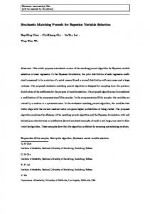
However, this result does not extend to all subsequent iterations. On the contrary, the offset term in Eqn. 57 may improve the accuracy of the atoms and the convergence speed by getting closer to the actual coefficient magnitudes. To see its effect clearly, consider the trivial example of a dictionary having 2 atoms each having 2 elements. Assume that the two atoms are as shown in Fig. 2. The known vector b has a unique representation in terms of these two atoms (vectors representing the sides of the parallelogram). Now the MP algorithm will identify atom a1 and a2 alternately and each iteration will reduce the residual error. The solution will converge to 1
If we use the terminology from the frame theory, such a condition is equivalent to saying that the atoms make a
tight frame [29].
17
(MP)
c2
r1(CMP)
a2 (CMP) c2
r1 (MP) r2 (MP) r3 (MP)
b a1
c1 (CMP) c1 (MP) Figure 2: CMP vs MP with two 2-D atoms. MP iterations consist of alternate orthogonal projections onto the two atoms, which converges to the sides of the parallelogram ultimately. CMP converges only in two iterations. the unique solution ultimately. The CMP algorithm, however, will find the true coefficients in 2 iterations. The offset term helps in finding the true coefficient of a1 in the first iteration. Though it makes the residual error larger than that of MP, the error is collinear with a2 . Therefore, the second iteration results in zero residual error. This example provides us some intuitive idea about how, in a general case, the CMP proceeds as against the MP. In general, we can expect a faster convergence and better sparsity compared to the MP.
4.2
OCMP versus OMP
Now let us consider the performance of OCMP in relation to that of OMP. At the first iteration, OCMP is the same as CMP and OMP is the same as MP. Therefore let us consider some jth iteration where j > 1. Now, since OCMP evolves from CMP and OMP evolves from MP, in light of the statements made above, it seems less likely to have the same set of selected atoms for both algorithms at the jth iteration. However, they perform an updating of the coefficients through orthogonal projection. Therefore the relative evolution of these two algorithms over iterations cannot be inferred in a straightforward manner from the evolutions of CMP and MP. Nevertheless we assume them to have the same set of selected atoms at the jth iteration because of the reasons given earlier. Let us consider the OCMP algorithm. As defined before, let Aj denote the matrix containing the selected atoms at iteration j. We can simplify the expressions for the complementary residual error and the coefficient vector following similar steps as we did for the CMP algorithm. The coefficient vector can be expressed as P cOCM j
= (ATj (AAT )−1 Aj )−1 ATj (AAT )−1 b.
And the resulting approximation error can be simplified as P P 2 P T T P 2 ²OCM = kb − Aj cOCM k = bT b − 2(cOCM ) Aj b + kAj cOCM k . j j j j
18
(59)
The coefficient vector and the residual error for OMP with the same set of atoms in the sparse solution are given as P cOM j
= (ATj Aj )−1 ATj b
(60)
P ²OM j
= bT (IK − Aj (ATj Aj )−1 ATj )b,
(61)
P = krOM P k2 , the residual error energy with OMP. Comparing these expressions, we where ²OM j j
can write: P cOCM j
P P = cOM + (ATj (AAT )−1 Aj )−1 ATj (AAT )−1 rOM j j
(62)
P ²OCM j
P P P 2 = ²OM + kAj (cOCM − cOM )k . j j j
(63)
Now, if the atoms make a tight frame, i.e., when AAT = tIK , t > 0, then the second term in the first equation above is equal to a null vector (the residual vector in OMP is orthogonal to the subspace spanned by the columns of Aj ). This means that both OCMP and OMP result in the same coefficients. Using this relationship in the second equation, we get identical residual error energy. It is easy to show that the complementary residual energy for any atom at a certain iteration is equal to the residual energy for the same atom with the same set of previously selected atoms. In other words, OMP and OCMP compare the same set of values for the selection of the atoms at each iteration. This results in identical coefficients and errors for both OCMP and OMP. Therefore, when the rows of A are orthogonal with identical norms, the OCMP is equivalent to the OMP. Further, we see that when the OMP identifies the atoms correctly leading to zero residual error, the OCMP also does the same. In the general case when the rows of A are not orthogonal with the same l2 norm, the above P is zero, then cOCM P expression provides interesting information. First of all, it shows that, if rOM j j P . This means that if OMP finds the exact solution, then the OCMP also gives is equal to cOM j
the exact solution if it identifies the same atoms as the OMP. This also shows that, in general, the approximation error with OCMP is not orthogonal to the subspace spanned by the selected atoms. As a result, the approximation error is more than that of the OMP algorithm. However, as for the residual error of CMP in relation to that of MP, this result of higher residual error may not extend to all subsequent iterations. Furthermore, the convergence can be faster provided the error aligns more closely with any of the remaining atoms. We also note here that the equivalence of MP and CMP or OMP and OCMP in the case of a tight dictionary is valid because of our use of l2 norm for minimizing the residual or complementary residual error. If we use some other norms, for example l1 or l∞ , the equivalence does not hold even if we use a tight dictionary. In this paper, we assume the use of l2 norm for all algorithms.
4.3
More on the residual error
With complementary algorithms, the increase in the approximation error at the first iteration is not unexpected since CMP searches for the sparse solution in a different space. This error can be derived in a straightforward manner using the selected atom instead of obtaining it from the 19
approximation of CMP. Let us assume that the actual sparse representation of b is given as b = p1 α1 + p2 α2 + · · · + pm αm ,
(64)
where m ≤ K, pi ’s are the coefficients of the atoms αi , 1 ≤ i ≤ m. All the matching pursuit algorithms first identify the best atom and then (or simultaneously) find its coefficient at each iteration. Suppose we have the identified atom α1 at the first iteration. Now we ask the following question: what is the value of its coefficient so that the l2 norm of the minimum l2 norm solution of the system of equations in Eqn. 1 with the resulting error as the observation vector is minimized (over all coefficient values) ? To answer this question, let us assume that α1 = ak . We can rewrite the above equation as follows b = cak + e,
(65)
where c denotes the unknown coefficient and e denotes the approximation error. This can be rewritten as e = b − cak . The minimum l2 norm solution of Ax = e is given as le = AT (AAT )−1 e = AT (AAT )(b − cak ) Taking the derivative of kle k2 ≡ lTe le with respect to c and making it equal to zero, we can solve for c as: c=
aTk (AAT )−1 b . aTk (AAT )−1 ak
(66)
This is exactly the coefficient given by the CMP after the first iteration if it selects ak as the best atom. If we had considered a later iteration, we would have substituted the resulting approximation error for b and we will still get the same coefficient value as given by the CMP. Now we can ask another related question: what is the value of the coefficient c so that the minimum l2 norm solution of the resulting error has a zero at the index corresponding to the index of α1 ? Having a zero at the corresponding index implies that at least in the minimum l2 norm solution, the contribution of α1 is zero. The kth element of the minimum l2 norm solution of e is given as aTk (AAT )−1 e = aTk (AAT )(b − cak ).
(67)
Making it equal to zero and solving for c, we get c=
aTk (AAT )−1 b . aTk (AAT )−1 ak
(68)
This is again the same solution as for the previous question. The resulting approximation error is therefore equal to the residual error of CMP. Let r1 denote the approximation error. It is easy to show that the minimum l2 norm solution of Ax = r1 is the complementary residual error of CMP with the atom ak identified at the first iteration. The above result also extends to the OCMP. Let us assume that we have identified the set of atoms αi , i = 1, 2, . . . j, up to the iteration number j. Taking these atoms as columns of matrix Aj , we can formulate the approximation as: b = Aj c + e, 20
where c denotes the vector of unknown coefficients. We can now ask two similar questions as before: (1) what is the value of c so that the l2 norm of the minimum l2 norm solution of Ax = e is minimized (over all coefficient values) ? and (2) what is the value of c so that the minimum l2 norm solution of Ax = e has zeros at indices corresponding to the indices of αi ’s , i = 1, 2, . . . , j? Following similar steps as above, we can show that the solution to both these problems is given as c = (ATj (AAT )−1 Aj )−1 ATj (AAT )−1 b. This is equal to the coefficient obtained by the OCMP algorithm. It follows that the residual error of OCMP is equal to the the resulting approximation error. It is easy to show that the minimum l2 norm solution for this error is equal to the complementary residual error of the OCMP when the OCMP identifies the same set of atoms. The above results show that the CMP and OCMP may converge faster and may have higher accuracies in selected atoms than the their classical matching pursuit counterparts. These results can also be intuitively predicted based on a simple observation: classical matching pursuit algorithms identify the best atom at any iteration by taking inner products which involve only individual atoms but not their inter-relationships. The complementary matching pursuit algorithms use the inter-relationships among the atoms in the form of the matrix AAT which exists in the computation of x2 . The results presented above corroborate the inclusion of this matrix product in the computation of the coefficients. We have not yet compared the complexities of the two different approaches. Proponents of the classical matching pursuit algorithms may immediately notice the matrix inversion operations in the computation of the complementary residual error and may complain that both CMP and OCMP will be much more compute-intensive than their classical counterparts. We must, however, remember that the expressions for the residual errors are direct representations of the actions we performed to get to the solution. As we showed in this section, the expressions for the complementary residual error and the coefficient can be simplified. In fact, what we showed in this section is that these terms can be directly computed from the dictionary matrix A instead of using the complementary matrix G. Besides, these expressions also show that the complementary algorithms are equivalent to classical matching pursuits done in the row-space of A, i.e., SA . This is presented in the next section.
5
Equivalence to MP in row-space
Let us consider our original system of equations: Ax = b. Since the atoms make a redundant basis for RK , AAT is an invertible matrix. As a consequence, the exact sparse solution to this system is also an exact sparse solution to the following system and vice versa; AT (AAT )−1 Ax = x2 ,
(69)
since AT (AAT )−1 b = x2 . Let φi ≡ AT (AAT )−1 ai , i ∈ I, denote the transformed set of atoms. Clearly these transformed atoms lie in the row-space of A. If we define a new dictionary matrix Φ 21
whose ith column is φi , then the above system of equations can be rewritten as Φx = x2 .
(70)
Notice that this system has the same number of equations as the number of unknowns (N ), but the matrix on the left side is rank-deficient. Furthermore, each atom no longer has unit norm. Let us consider applying MP to find the sparse solution to this system of equations. The projection error φ φT
φ φT
with atom φi is given as (IN − kφi i ki2 )x2 , and hence the l2 norm of the error is (x2 )T (IN − kφi i ki2 )x2 . Substituting the expressions for x2 and φi , we get kx2 k2 −
(x2 [i])2 T )−1 a (AA aT i i
after simplification. This
expression is identical to the expression for the complementary residual error in Eqn. 49. Therefore the two algorithms compare the same set of values for finding the optimal values. Let ak be the atom with the minimum projection error. The coefficient of ak is φTk x2 aTk (AAT )−1 b = . kφk k2 aTk (AAT )−1 ak
(71)
This expression is identical to the expression for the coefficient with the CMP in Eqn. 52. Since the resulting residual errors after the first iteration are same, the algorithms also identify the same atom in the second iteration with the same coefficient values leading to the same residual error and so on. In other words, these two approaches produce the same sparse approximations. Following similar steps as above, it is easy to show that the application of OMP/OOMP on this system of equations is equivalent to the application of OCMP/OOCMP on the original system of equations. Therefore, instead of applying (O/OO)CMP on the original system, we can simply apply the classical (O/OO)MP on this modified system. This has two advantages: first it shows that we do not need the G matrix. Secondly, the complexity of the (O/OO)CMP on the modified system is of the same order as that of (O/OO)MP on the original system except that the former approach deals with N dimensional vectors and the vectors are not normalized. Now, applying the (O/OO)CMP through this modified system looks so simple. However, it would not provide us the intuitive understanding of the ”complementarity” and the convergence if we had started from this modified system of equations.
6
Summary
Let us now provide a conceptual summary of CMP in relation to MP. Fig.3(a) shows that the dictionary matrix A maps the RN to its column-space. The nullspace of A is mapped to 0K in the column space and the solution space2 {x : Ax = b} is mapped to b. The atoms ai , i ∈ I, lie in the column-space. At each iteration, the MP algorithm finds the point closest to b among N points (one point per atom) and moves there. Therefore, at each iteration, the approximation moves closer to b and thus the approximation error becomes lesser. Corresponding to each approximation point, there is a point in RN that approximates the solution vector x. As the approximation gets closer to 2
The solution space is not a vector space since it does not contain the null vector. It can be obtained by adding
a vector in the solution space to all the vectors in the nullspace.
22
nullspace of
A
nullspace of
0
columnspace of
A
0
0
columnspace of
A
0
x1 x2
A
b1
b2 b3
x3
x0
b1
x3
x1
x0
x2 b
b2 b
δ
solution space
b3
x2
x2
solution space
δ
N
N
R
R
(a) MP
(b) CMP
Figure 3: Vector space representation of the sparse approximation by MP and CMP b, these points in RN get closer to the solution space. These points are all sparse. The algorithm terminates when the approximation is sufficiently close to b. The resulting sparse solution is close to the solution space. Fig. 3(b) shows the action of CMP. At each iteration, the CMP algorithm finds the point closest to the solution space among N points (one point for each atom) and moves there. Therefore, at each iteration, the sparse vector x moves closer to the solution space and thus the complementary residual error becomes lesser. Corresponding to each sparse vector, there is an approximation in the column space. As x gets closer to the solution space, the approximation point in the column space get closer to b. The algorithm terminates when the approximation is sufficiently close to b. The set of sparse points in RN and the corresponding set of approximation points in the columns space are not necessarily the same as those with the MP because of different criteria applied by the two algorithms for choosing the best point among N points at each iteration. However, when the dictionary is tight, these two sets of points for both algorithms match exactly. The complementarity of CMP is seen from the fact that the sparse points chosen by the algorithm are actually obtained from the solution space. The algorithms finds N points in the solution space by adding x2 to N points inside the nullspace. Then it finds the N sparse points which are closest to each of these points, and among these N sparse points it selects the one which is the closest to the corresponding point in the solution space. In other words, the algorithm moves from the solution space to the nearest sparse vector at each iteration (it searches for ’the sparse vector among the solution vectors’). As the iteration proceeds, the sparse points come closer and closer to the solution space. In contrast to this, the MP algorithm moves towards the solution space always keeping the points sparse (it searches for ’the solution vectors among the sparse vectors’). The actions of the orthogonal extensions to MP/CMP can be easily understood by referring to Fig. 3(a)/3(b) Note that the (OO/O)CMP can stop at some iteration if the distance between the latest sparse point and the solution space is sufficiently small. However, the stopping criterion in the original problem is defined with the approximation error δ. Therefore the (OO/O)CMP has to map the resulting sparse point to the column space and then check for the approximation error. On the
23
other hand, this constraint suggests that there is a scope for improving the performance of the (OO/O)CMP. We have observed that the approximation errors resulting from the (OO/O)CMP is not orthogonal to the immediately selected atom (subspace spanned by all the selected atoms). This is also true for the last iteration, if the approximation error is nonzero. Once the atom has been identified, the best approximation with it is the orthogonal projection of the residual error on it (as in MP), and the best approximation with all the selected atoms is the orthogonal projection of the residual onto the subspace spanned by them. Therefore, once the best atom has been identified in (OO/O)CMP, we can compute the best approximation with it (the set of all selected atoms) through orthogonal projection and compute the resulting approximation error. If the approximation error is below the desired threshold, the algorithm can terminate; otherwise we compute the approximation as given by the (OO/O)CMP and then move to the next iteration. For the simulation results reported in this paper, we do not make this change in the complementary MPs in order that we maintain ”full complementarity” and the same order of complexity as the classical MPs.
7
Simulation Results
In order to compare the different sparse algorithms, we performed two experiments with a dictionary of 55 atoms each having 32 elements. We used the recently proposed K-SVD algorithm [30] to derive the dictionary atoms. The K-SVD algorithm comprises two steps for designing a dictionary from a set of training signals. In the first step, it sparse-codes the training set using an initial dictionary and any sparse coding algorithm. In the second step it updates the dictionary atoms using an SVD based K-means algorithm on the sparse-coded data. In [30], the authors have used OMP as the sparse coding algorithm because of its lower complexity. We used the K-SVD code available by the authors of [30] with a training set of 1500 signals. Except the dictionary parameters chosen as above, all other parameters were kept unchanged. The derived dictionary matrix had normalized atoms and its rows were non-orthogonal. In the first experiment, we compared the convergence of CMP, OCMP, and OOCMP with that of MP, OMP and OOMP algorithms. By taking linear combinations of 5 and 8 randomly selected atoms, we generated in each case a test set of 10000 signal vectors. The weights of the atoms were randomly generated using a Gaussian random variable with mean zero and variance 1. We sparse-coded these signal vectors with different algorithms without any error bound and without any limit on the maximum number of identified atoms. Fig. 4 shows the mean square residual errors for different algorithms at different number of iterations. The mean was computed over all 10000 signal vectors and then it was normalized with respect to the mean signal energy. We observe that, after some initial few iterations, the error with the CMP decreases at a faster rate than with the MP. Therefore it will converge faster than the MP if we set a very small threshold for convergence. When the signals are generated from 5 atoms, the errors with the OCMP and OOCMP reach much lower values than with the OMP and OOMP at the 5th iteration. Similarly with 8 generating atoms, the OCMP and OOCMP attain much lower error values than the OMP 24
0
0 MP OMP OOMP CMP OCMP OOCMP
Mean square approximation error [dB]
−10
−15
−10
Mean square approximation error [dB]
−5
−20
−25
−30
−35
−20
−30
−40
MP OMP OOMP CMP OCMP OOCMP
−40 −50 −45
−50
0
1
2
3
4
5 6 No of iterations
7
8
9
10
−60
0
2
4
6
8 No of iterations
10
12
14
16
Figure 4: Residual energy for different number of iterations. Number of generating atoms: 5 (left) and 8 (right). and OOMP at the 8th iteration. The residual error with (O)OMP/(O)OCMP relative to that with MP/CMP is expected. In the second experiment, we varied the number of generating atoms from 1 to 16, and in each case generated 10000 signal vectors as input signals. As in the previous experiment, the generating atoms were randomly selected and their weights were randomly generated from a Gaussian random variable with mean zero and variance one. In the sparse coding algorithms, we specified an error bound of 10−3 per component and a maximum limit of 16 atoms in the approximation. Besides the matching pursuit algorithms, we also implemented the BP algorithm [6]. In order to provide a fair comparison with the other algorithms, we modified the BP algorithm for the above bounds. First, based on the usual BP solution, we sorted the atoms in the decreasing order of their weight magnitudes. Then we selected the first k atoms, k ≤ 16 and computed the coefficients using the pseudoinverse of the matrix containing only these atoms. If the resulting residual error was lower than the error bound, we terminated the iteration, otherwise we incremented k and repeated the procedure provided k was less than or equal to 16. Therefore, in the modified BP, we selected the atoms based on the magnitudes of their weights given by the BP, but determined their coefficients by the pseudoinverse. We compared the algorithms in terms of (i) sparsity, i.e., the number of atoms identified, (ii) the approximation accuracy or the residual error, (iii) the accuracy of detecting the generating atoms, and (v) the accuracy of coefficients with truly detected atoms. Fig. 5 displays the number of atoms identified by different algorithms. We observe that the CMP produces sparser approximation than the MP for 4 or more generating atoms. Among all the algorithms, the OCMP and the OOCMP produce the best sparsity results. The improvements over other algorithms are more pronounced as the number of generating atoms is made higher. Note that the plots tend to saturate because of the specified maximum of 16 atoms in the approximation. Fig. 6 shows the mean square error resulting from different algorithms. We see that the CMP yields lower residual error than the MP for 6 or more generating atoms. The OCMP and OOCMP result in the least error among all the algorithms. The relative gain over the OMP/OOMP becomes more 25
16 0.012 MP OMP OOMP CMP OCMP OOCMP BP
14
12 mean square residual error
No of atoms in the sparse representation
0.01
10
8
MP OMP OOMP CMP OCMP OOCMP BP
6
4
0.008
0.006
0.004
0.002
2 2
4
6 8 10 No of generating atoms for the signal
12
14
0
16
Figure 5: No of atoms identified versus the number of actual atoms. Error bound
δ2
=
32 × 10−6 ,
maximum 16 atoms.
2
4
6 8 10 No of generating atoms for the signal
12
14
Figure 6: Mean square residual error versus the number of atoms. Error bound δ 2 = 32 × 10−6 , maximum 16 atoms.
pronounced as the number of generating atoms is increased. Fig. 7 displays the fraction of true atoms identified. It is interesting to see that the CMP identifies more correct atoms than not only MP, but also OMP. However, the OCMP and OOCMP outperform all of them including BP. Again the relative improvements are more pronounced for a higher number of generating atoms. Fig. 8 shows the relative frequencies of coefficient differences for truely identified atoms when the number of generating atoms is 16. A value of zero difference indicates that the computed coefficient is identical to the true coefficient used in the linear combination to generate the signal. Therefore a higher relative frequency at zero with smaller variance implies higher accuracy of computed coefficients. Fig. 8 shows that the CMP produces more accurate coefficients than the MP. The coefficients given by OCMP (OOCMP) are closer to the original coefficients than those of OMP (OOMP). Even OCMP and OOCMP both yield closer coefficients than the BP. If we compare the three figures, we observe that the relative performance of different algorithms is similar to their relative sparsity and residual error performances. Recall that the BP guarantees the unique sparse solution when the number of atoms in the linear sum is below a certain bound. Therefore the relative performance of the BP in this experiment is not surprising.
8
Conclusions
In this paper, we have introduced the concept of a complementary matching pursuit for sparse coding. The basic CMP algorithm is similar to the classical MP algorithm but performs sparse coding through the complementary action of discarding atoms from the approximation. We showed that while the MP algorithm proceeds by minimizing the approximation error at each iteration, the CMP proceeds by minimizing the distance of the sparse vector from the solution space of the given linear system. As a consequence, the CMP converges towards the solution space while the 26
16
1
0.95
Fraction of correctly identified atoms
0.9
0.85
0.8
0.75 MP OMP OOMP CMP OCMP OOCMP BP
0.7
0.65
0.6
0.55
2
4
6 8 10 No of generating atoms for the signal
12
14
16
Figure 7: Fraction of correct atoms detected versus the number of atoms. Error bound δ 2 = 32 × 10−6 , maximum 16 atoms.
MP converges towards the specified signal to be sparse coded. We also showed that when the atoms make a tight frame, the CMP yields exactly the same approximation as the MP. We developed the orthogonal extensions of the CMP following the same lines as the MP’s extension to OMP and OOMP. The OCMP and OOCMP remove the suboptimality of the CMP by updating the approximation based on all selected atoms up to a given iteration. As a result they select a new atom at each iteration and converge faster. Like the CMP, they converge towards the solution space of the given linear system, thus the approximation error at each iteration may not be minimized. Furthermore, when the atoms make a tight frame, they yield identical sparse coding as their classical matching pursuit counterparts. We also showed that the CMP and its orthogonal extensions are equivalent to the MP and its orthogonal extensions respectively for a modified system of equations where the atoms and the given signal vector to be sparse coded are replaced in the modified system by their minimum l2 norm representations. The simulation results showed that the presented algorithms not only converge faster but also produce more accurate solutions with less approximation errors. Throughout the paper we have assumed that the observed signal b is a pure sparse linear sum of atoms without any additive noise. When the signal is observed with noise, the complementary matching pursuit algorithms can be very sensitive to the presence of the noise unless the noise is very small. This can be intuitively understood from the fact that these algorithms search for sparse solutions among the solution vectors to the given under-determined system. When the observations are accompanied by noise, the solution space gets perturbed. As a result, the algorithms will be searching for the sparse vector among solution vectors which belong to the perturbed solution space. The perturbation of the solution space is dependent not only on the noise amount but also on the dictionary matrix A (in the form of the stability of the matrix (AAT )−1 ). Since most of the practical applications involve noisy observations, it is important to investigate these algorithms for noisy signals and to develop techniques to circumvent the stability issues. From the theoretical point 27
0.9
0.9 MP CMP BP
0.7
0.7
0.6
0.6
0.5
0.4
0.5
0.4
0.3
0.3
0.2
0.2
0.1
0.1
0 −2
−1.5
−1 −0.5 0 0.5 1 Coefficient difference for correctly identified atoms
1.5
OMP OCMP BP
0.8
Relative frequency
Relative frequency
0.8
2
0 −2
−1.5
−1 −0.5 0 0.5 1 Coefficient difference for correctly identified atoms
1.5
2
0.9 OOMP OOCMP BP
0.8
0.7
Relative frequency
0.6
0.5
0.4
0.3
0.2
0.1
0 −2
−1.5
−1 −0.5 0 0.5 1 Coefficient difference for correctly identified atoms
1.5
2
Figure 8: Relative frequency of coefficient difference for matching atoms for 16 generating atoms. Error bound δ 2 = 32 × 10−6 , maximum 16 atoms. of view, it is important to analyze the convergence and the sparsity of the presented algorithms with noisy observations. In addition, it is also interesting to investigate the convergence and the sparsity of the presented algorithms vis-`a-vis their classical counterparts in a precise manner. The results presented here considered a dictionary of a fixed size. Since the dimension of the subspace c depends on the size of the dictionary, the convergence and the sparsity of the complementary SA
algorithms are expected to be increasingly better as the size of the dictionary increases. Future research will be directed to these extensions.
References [1] B. K. Natarajan, “Sparse approximate solutions to linear systems,” SIAM J. Comput., Vol. 24, No. 2, pp. 227–234, Apr. 1995. [2] G. Davis, S. Mallat, and M. Avellaneda, “Adaptive greedy approximations,” J. Constr. Approx., Vol. 13, pp. 57-98, 1997.
28
[3] S. Mallat and Z. Zhang, “Matching pursuits with time-frequency dictionaries,” IEEE Trans. Signal Process., Vol. 41, No. 12, pp. 3397–3415, 1993. [4] Y. C. Pati, R. Rezaiifar, and P. S. Krishnaprasad,“Orthogonal matching pursuit: Recursive function approximation with applications to wavelet decompositions,” Proc. 27th Asilomar Conf. on Sig., Sys. and Comp., Vol. 1, Nov. 1993. [5] G. Davis, S. Mallat, and Z. Zhang, “Adaptive time-frequency decompositions with matching pursuits,” Proc. SPIE, Wavelet Applications, H. H. Szu, Ed, Vol. 2242, pp. 402–413, 1994. [6] S. S. Chen, D. L. Donoho, and M. A. Saunders,“Atomic decomposition by basis pursuit,” SIAM J. Sci. Comput., Vol. 20, No. 1, pp. 33–61, 1988. [7] G. Harikumar, C. Couvreur, and Y. Bresler, “Fast optimal and suboptimal algorithms for sparse solutions to linear inverse problems,” Proc. IEEE ICASSP, pp. 1877-1881, 1998. [8] C. Couvreur and Y. Bresler, “On the optimality of the backward greedy algorithm for the subset selection problem,” SIAM J. Mat. Anal. and Appls, Vol. 21 , No. 3 pp. 797–808, Feb.Mar. 2000. [9] S. J. Reeves, “An efficient implementation of the backward greedy algorithm for sparse signal reconstruction,” IEEE Signal Process. Lett., Vol. 6, No. 10, pp. 266–268, Oct. 1999. [10] S. F. Cotter, K. K.-Delgado, and B. D. Rao, “Efficient backward elimination algorithm for sparse signal representation using overcomplete dictionaries,” IEEE Signal Process. Lett., Vol. 9, No. 5, pp. 145–147, May 2002. [11] J. A. Tropp and A. C. Gilbert, “Signal recovery from random measurements via orthogonal matching pursuit,” IEEE Trans. Inform. Theory, Vol. 53, No. 12, pp. 4655–4666, Dec. 2007. [12] J. Tropp, “Greed is good: algorithmic results for sparse approximation,” IEEE Trans. Inform. Theory, Vol. 50, No. 10, pp. 2231–2242, 2004. [13] L. Rebollo-Neira and D. Lowe, “Optimized orthogonal matching pursuit approach,” IEEE Signal Process. Lett., Vol. 9, No. 4, pp. 137–140, 2002. [14] D. L. Donoho and X. Huo,“Uncertainty principles and ideal atomic decompositions,” IEEE Trans. Inform. Theory, Vol. 47, No. 11, pp. 2845–2862, Nov. 2001. [15] D. L. Donoho, “For most large underdetermined systems of linear equations the minimal l1 norm solution is also the sparsest solution,” Comm. Pure Appl. Math., Vol. 59, No. 6, pp. 797–829, 2006. [16] M. Elad and A. M. Bruckstein, “A generalized uncertainty principle and sparse representation in pairs of bases,” IEEE Trans. Inform. Theory, Vol. 48, No. 9, pp. 2558–2567, Sept. 2002.
29
[17] R. Gribonval and M. Nielsen, “Sparse representations in unions of bases,” IEEE Trans. Inform. Theory, Vol. 49, No. 12, pp. 3320-3325, Dec. 2003. [18] D. M. Malioutov, M. etin, and A. S. Willsky, “Optimal sparse representations in general overcomplete bases,” Proc. IEEE ICASSP, Montreal, May 2004. [19] M. Elad, “Sparse representations are most likely to be the sparsest possible,” EURASIP J. on Appl. Signal Process. Vol. 2006, No. 1, pp. 1–12, Jan. 2006. [20] J.-J. Fuchs, “On sparse representations in arbitrary redundant bases,” IEEE Trans. Inform. Theory, Vol. 50, No. 6, pp. 1341-1344, Jun. 2004. [21] J. J. Fuchs, “Recovery of exact sparse representations in the presence of bounded noise,” IEEE Trans. Inform. Theory, Vol. 51, No. 10, pp.3601–3608, 2005. [22] J. A. Tropp, “Just relax: Convex programming methods for identifying sparse signals,” IEEE Trans. Inform. Theory, Vol. 51, No. 3, pp. 1030–1051, Mar. 2006. [23] I. F. Gorodnitsky and B. D. Rao, “Sparse Signal Reconstruction from Limited Data Using FOCUSS: A Re-weighted Minimum Norm Algorithm,” IEEE Trans. Signal Process., Vol. 45, No. 3, pp. 600–616, Mar. 1997. [24] B. D. Rao and K. K.-Delgado, “Deriving algorithms for computing sparse solutions to linear inverse problems,” Proc. 31st Asilomar Conf. Sig., Sys. and Comp., Vol. 1, pp. 955–959, 1998. [25] B. A. Olshausen and D. J. Field, “Sparse coding with an overcomplete basis set: a strategy employed by VI?,” Vision Res., Vol. 37, pp. 3311–3325, 1997. [26] M. S. Lewicki and B. A. Olshausen, “A probabilistic framework for the adaptation and comparison of image codes,” J. Opt. Soc. Amer. A: Opt., Image Sci. Vision, Vol. 16, No. 7, pp. 1587–1601, 1999. [27] D. L. Donoho, M. Elad, and V. Temlyakov, “Stable recovery of sparse overcomplete representations in the presence of noise,” IEEE Trans. Inform. Theory, Vol. 52, No. 1, Jan. 2006. [28] C. D. Meyer, Matrix Analysis and Applied Linear Algebra, SIAM, 2000. [29] V. K. Goyal, M. Vetterli, and N. T. Thao, “Quantized overcomplete expansions in RN : Analysis, synthesis, and algorithms, IEEE Trans. Inform. Th., Vol. 44, No. 1, pp. 16–31, Jan. 1998. [30] M. Aharon, M. Elad, and A. Bruckstein, “K-SVD: An algorithm for designing overcomplete dictionaries for sparse representation,” IEEE Trans. Signal Process., Vol. 54, No. 11, pp. 4311– 4322, 2006.
30