Jan 8, 2014 - the entanglement created by the interaction between the system observed and the .... the monogamy principle [22], S must be completely un-.
Complementary sequential measurements generate entanglement Patrick J. Coles1 and Marco Piani2
arXiv:1305.3442v2 [quant-ph] 8 Jan 2014
1
Centre for Quantum Technologies, National University of Singapore, 2 Science Drive 3, 117543 Singapore 2 Institute for Quantum Computing and Department of Physics and Astronomy, University of Waterloo, N2L3G1 Waterloo, Ontario, Canada We present a new paradigm for capturing the complementarity of two observables. It is based on the entanglement created by the interaction between the system observed and the two measurement devices used to measure the observables sequentially. Our main result is a lower bound on this entanglement and resembles well-known entropic uncertainty relations. Besides its fundamental interest, this result directly bounds the effectiveness of sequential bipartite operations—corresponding to the measurement interactions—for entanglement generation. We further discuss the intimate connection of our result with two primitives of information processing, namely, decoupling and coherent teleportation.
Heisenberg’s uncertainty principle [1] tries to capture one of the fundamental traits of quantum mechanics: the complementarity of observables like position and momentum. There are several variants of the principle which may be considered conceptually very different [2]. For example, one can consider the uncertainty related to the independent measurement of two observables, with the measurements performed on two independent but identically prepared quantum systems. In this scenario, the uncertainty principle for complementary observables can be understood as stating that there is an unavoidable uncertainty about the outcomes of the associated measurements. Alternatively, one can consider the sequential measurement of such two observables, performed on the same physical system. In this case, the uncertainty principle is understood as the unavoidable disturbance on the second observable due to the measurement of the first. Although this latter disturbance-based interpretation of the principle is the one originally considered by Heisenberg in his famous γ-ray thought experiment [3], researchers have more often focussed on the first scenario. Unavoidable uncertainty was stated quantitatively by Kennard [4] and Robertson [5] in the famous uncertainty relation involving standard deviations. Since then, uncertainty relations have been cast in information-theoretic terms [6]. For example, a well-known entropic uncertainty relation is that of Maassen and Uffink [7]. Working in finite dimensions, they consider two orthonormal bases {|Xj i} and {|Zk i} for the Hilbert space HS of a quantum system S, to which one can associate observables X and Z, respectively. For any state ρS , they find H(X) + H(Z) > log(1/c), P
(1)
where H(X) := − j p(Xj ) log p(Xj ) is the Shannon entropy associated with the probability distribution p(Xj ) := hXj |ρS |Xj i (similarly for H(Z)), logarithms are taken in base 2, and c := maxj,k |hXj |Zk i|2 quantifies the complementarity between the X and Z observables. The r.h.s. of (1) vanishes when X and Z share an eigenstate. At the other extreme, when X and Z are complementary—so-called mutually unbiased bases (MUBs) with |hXj |Zk i|2 = 1/d, ∀j, k, and
d = dim(HS )—the r.h.s. becomes log d. In the latter case, Eq. (1) implies that when our uncertainty about X approaches zero, our uncertainty about Z must approach its maximum value log d. In this Letter, we offer a novel view on what complementarity entails by relating it to another fundamental trait of quantum mechanics: entanglement [8]. In [9] it was already proved that an entropic uncertainty relation like (1) has a correspondent entanglement certainty relation. In more detail, Ref. [9] considers the generation of entanglement between measurement devices and independent, although identically prepared, copies of some physical system, and proves that, when dealing with complementary observables, there is unavoidable creation of entanglement between at least one copy of the system and one measuring device. Here, as Heisenberg did originally, we instead consider sequential measurements performed on the same physical system, rather than independent copies of the system; on the other hand, following [9–13], we still focus on the entanglement generated between the system and the measurement devices. In general, for any X and Z, we can lower-bound the entanglement E(X, Z) between the system and the measurement devices created from sequentially measuring X and Z with E(X, Z) > log(1/c),
(2)
where the c factor appearing here is precisely the same c appearing in Eq. (1), and we provide more details on how we quantify entanglement in the following. Besides the fact that our approach connects in a fundamental way two basic properties of quantum mechanics, complementarity—in the sequential-measurement scenario—and entanglement, our results have also direct operational interpretations. On one hand, they provide bounds on the usefulness of sequential bipartite operations—corresponding to the measurement interactions—for entanglement generation. On the other hand, we argue below that our analysis is directly linked to the quantum information processing primitives of decoupling [14–18] and coherent teleportation [19, 20]. Setup.—The basic setup corresponding to our main result is given in Fig. 1. The system is initially described
2 (0)
by some arbitrary density operator ρS . It first interacts with a device M1 meant to measure the observable X. We depict this interaction with the controlled-NOT (CNOT) symbol, although more generally it represents P j a controlled-shift unitary, UX = j [Xj ] ⊗ S ⊗ 11M2 , actingPon the tripartite Hilbert space HSM1 M2 , where S = k |k + 1ihk| is the shift operator and [Xj ] is a shorthand notation for the dyad |Xj ihXj |. This is a unitary model for the measurement process [21]. After this, the system interacts with a second device M2 , which measures the Z observable; the unitary is given P by UZ = j [Zj ] ⊗ 11M1 ⊗ Sj . We suppose that both M1 and M2 are initially in the |0i state, although later in the article we consider the effect of relaxing this assumption. We denote the states at times t0 , t1 , and t2 in Fig. 1 as (2) (1) (0) ρSM1 M2 , ρSM1 M2 , and ρSM1 M2 , respectively. Entanglement generation.—We focus on the bipartite entanglement E(X, Z) between S and the joint system M1 M2 present in the final state X (2) (0) ρSM1 M2 = [Zl ][Xj ]ρS [Xk ][Zm ] ⊗ |jihk| ⊗ |lihm|. j,k,l,m
For concreteness we consider E to be the distillable entanglement [8], i.e., the optimal rate for distilling Einstein-Podolsky-Rosen (EPR) pairs (|0i|0i + √ |1i|1i)/ 2 using local operations and classical communication (LOCC) in the asymptotic limit of infinitely many copies of the state. However, our result holds for several other entanglement measures, because distillable entanglement is itself a lower bound for such measures [8]. Consider first the case where X and Z are MUBs. (2) In this case, ρSM1 M2 is maximally entangled across the (0)
S:M1 M2 cut, regardless of the system’s initial state ρS . One can see this by noting that, if we choose the LOCC operation that measures M1 in the standard basis and communicates the result to the party holding S, the resulting conditional pure state on SM2 is, up to an irrelevant local change of basis, √ a maximally entangled e-dit Pd−1 of the form i=0 |ii|ii/ d. Alternatively, and more elegantly, we can factor out a maximally entangled state simply by performing a local unitary on M1 M2 ; more precisely, the following holds. Proposition 1. Let X and Z be MUBs. Define HM1 = P j P ⊗ controlled unitary UM1 M2 = j σX j |Xj ihj| and the √ P j [j], where σX := d k hXk |Zj i[Xk ]. Then (2)
(0)
† † UM1 M2 HM1 ρSM1 M2 HM UM = [Φ]SM2 ⊗ (ρS )M1 , 1 1 M2 (3) √ P with |Φi = ( j |Zj i|ji) d: the local unitary UM1 M2 HM1 (2)
applied to ρSM1 M2 leaves M1 in the system’s initial state (0)
ρS , and SM2 maximally entangled. Thus, in the case of MUBs, we can identify several tasks that are accomplished by sequentially measuring X and Z as in Fig. 1. Besides producing maximal en-
(0)
ρS
|0i |0i
S
t0
X
t1
Z t2
M1 M2
FIG. 1: Circuit diagram for the sequential measurement of the X and Z observables on system S.
(0)
tanglement, the state ρS is “teleported” from the system to the measurement devices. Indeed, the protocol we have described above is commonly known as coherent teleportation [19, 20]. Furthermore, since S is maximally entangled to M1 M2 at the end of the protocol, then, by the monogamy principle [22], S must be completely uncorrelated with any other system S ′ . The procedure of performing an operation on S to destroy its potential correlations with S ′ is known as decoupling [14–18]. Our main contribution is to extend the above discussion to the case where X and Z have partial complementarity (c > 1/d): Can we still create entanglement, coherently teleport, and decouple even if X and Z are not MUBs, and if so, to what degree? Our main result (2), says that, as soon as there is partial complementarity between X and Z, some distillable (2) entanglement is present in ρSM1 M2 . Theorem 2. Let E(X, Z) denote the distillable entanglement between S and M1 M2 at time t2 in Fig. 1. Then (2) holds. Proof. We give two alternative proofs. The first is based on the uncertainty principle with quantum memory [23] and the second is based on the monotonicity of entanglement under LOCC [8]. The second proof approach yields a slightly stronger version of (2). In the first approach we we apply the uncertainty principle with quantum memory [23] at time t1 (just after the X measurement) to get: H(X|M1 M2 )ρ(1) + H(Z|S ′ )ρ(1) > log(1/c) (0)
(4)
where we let S ′ purify the initial state ρS , and where the first and second terms in (4) are the conditional enP (1) (1) (1) tropies of ρXM1 M2 := j [Xj ]ρSM1 M2 [Xj ] and ρZS ′ := P (1) k [Zk ]ρSS ′ [Zk ] respectively. The von Neumann conditional entropy of σ is defined as H(A|B)σ := H(σAB ) − H(σB ), with H(σ) = −Tr(σ log σ) the von Neumann entropy. Because X was already measured by M1 , we have H(X|M1 M2 )ρ(1) = 0. Also, from a result in [9, 24], we have H(Z|S ′ )ρ(1) = E(X, Z), completing the proof. In the second approach, we note that the final entanglement is larger than the average entanglement obtained from measuring M1 in the standard basis followed by communicating the result to the party holding system
3 P (2) S. That is, E(X, Z) > j pj H(ρS,j ), where we used that the conditional states associated with different mea(2) surement outcomes are bipartite pure states, pj ρSM2 ,j = (2)
TrM1 [(11 ⊗ |jihj| ⊗ 11)ρSM1 M2 ], hence their entanglement (2) ρS,j
(2) TrM2 (ρSM2 ,j ).
= is the entropy of the reduced state We obtain X pj H({|hXj |Zk i|2 }k ), E(X, Z) >
(5)
j
where the entropy on the r.h.s. is the classical entropy of the set of overlaps obtained from varying the index k. Equation (5) is slightly more complicated than (2) because it depends on the initial state through the prob(0) abilities pj = hXj |ρS |Xj i. On the other hand, it is slightly stronger, implying (2) by noting that Shannon entropy upper-bounds the min-entropy Hmin ({qk }) = − log maxk qk , and averaging over j in (5) yields a larger value than minimizing over j, completing the proof. So, even for limited complementarity, the circuit in Fig. 1 still generates entanglement “efficiently”. Using our main result, we also prove below that decoupling and coherent teleportation are approximately achieved in the case of approximate complementarity. We further consider two generalizations of our results: to the case of mixed measurement devices, and to the case of an arbitrary number of sequential measurements.
H(S|M1 M2 )ρ(2) + H(S|S ′ )ρ(2) > 0 because of strong subadditivity of entropy [28]. Finally, note that log d − H(S|S ′ )ρ(2) is the relative entropy on the l.h.s. of (6). If X and Z are complementary, c = 1/d and Corol(2) (2) lary 3 implies ρSS ′ = 11/d ⊗ ρS ′ . More generally, (6) ′ shows that S and S are almost decoupled if X and Z are almost complementary. Coherent teleportation.—When X and Z are MUBs, Proposition 1 says that there exists a local unitary on (0) M1 M2 that recovers the input state ρS . As we decrease the complementarity between X and Z, the channel E : S(t0 ) → S(t2 ) goes from the completely depolarizing channel to the dephasing channel (in the limit X = Z), while the complementary channel E c : S(t0 ) → M1 M2 (t2 ) goes from a perfect quantum channel to a dephasing channel. One can therefore consider the quantum capacity of E c , i.e., the optimal rate at which E c allows for the reliable transmission of quantum information [29], as a measure of the complementarity of X and Z. We make these ideas quantitative in the following corollary. Corollary 4. The quantum capacity Q(E c ) of the channel E c satisfies Q(E c ) > log(1/c). Furthermore, there exists a recovery map �R such that the entanglement fi� c c delity Fe (R◦E ) := Tr [Φ]SS ′ (R◦E )S ([Φ]SS ′ ) is lowerbounded by Fe (R ◦ E c ) > 1/(d · c). (0)
Decoupling.—Decoupling [14–18] consists in transforming an arbitrary bipartite state ρSS ′ into some tensor product σS ⊗ σS ′ , and it has specific applications in state merging [25] and quantum cryptography [26]. Decoupling strategies often involve a local operation performed on system S only. Note that the effect on S of the circuit of Fig. 1 is equivalent to a random unitary channel P (0) k l † (0) k l σX ) , consisting of d2 σX )ρS (σZ ρS 7→ (1/d2 ) k,l (σZ unitaries each of P which is a product of generalized Pauli P operators, σX = j ω j |Xj ihXj | and σZ = j ω j |Zj ihZj | with ω = e2πi/d . It is well-known that when X and Z (0) (2) (2) are MUBs this results in ρSS ′ 7→ ρSS ′ = 11/d ⊗ ρS ′ . Can we guarantee approximate decoupling when X and Z exhibit only approximate complementarity? Because of monogamy of correlations, this question is closely related to the question of whether the X and Z measurements create entanglement [18]: if S is highly entangled to M1 M2 , then it is almost completely decoupled from some other system S ′ . Thus, (2) must imply a corresponding decoupling result. To prove this, we consider the relative entropy distance D(σkτ ) := Tr(σ log σ) − Tr(σ log τ ) [45]. We find the following. (0) Corollary 3. For any initial ρSS ′ , at time t2 (2)
(2)
D(ρSS ′ ||11/d ⊗ ρS ′ ) 6 log(d · c). (2)
(6)
Proof. The state ρSM1 M2 falls into a class of states [9, 27] for which the distillable entanglement satisfies E(X, Z) = −H(S|M1 M2 )ρ(2) . Moreover,
Proof. Suppose ρS = 11/d = TrS ′ [Φ]SS ′ ; then from (2), log(1/c) 6 E(X, Z) = −H(S|M1 M2 )ρ(2) (2)
(2)
= H(ρM1 M2 ) − H(ρS ),
(7) (2)
where the second equality follows from H(ρSM1 M2 ) = (0)
(2)
H(ρS ) = H(ρS ). The third line is a lower bound on the quantum capacity of the channel E c [29]. The proof of the second claim follows from the operational meaning of the conditional minentropy [30] Hmin (A|B)σ = − log[dim(HA ) maxR hΦ|(I ⊗ R)(σAB )|Φi], where the max is over all completelypositive trace-preserving maps R, which gives −H (S ′ |M1 M2 )ρ(2) , where S ′ maxR Fe (R ◦ E c ) = (1/d)2 min (0) ′ purifies ρS . Finally note that −Hmin (S |M1 M2 )ρ(2) > −H(S ′ |M1 M2 )ρ(2) = E(X, Z). Corollary 4 allows us to say that we can approximately (0) teleport the state ρS when X and Z are almost MUBs. Conceptually, Corollary 4 follows from (2) since the latter says that S becomes highly entangled to M1 M2 , which (2) implies that ρS must be close to the maximally mixed (0) state regardless of the input ρS , which implies that E is a bad channel and hence the complementary channel E c must be good [31]. Initially mixed devices.—In Fig. 1, we assumed the ini(0) tial states of the measurement devices were pure, ρM1 =
4 (0)
|0ih0| and ρM2 = |0ih0|. We now focus on the effects of mixing. While we still assume that the system-device interaction takes place on a time scale on which coherence is preserved, it is natural to restrict our attention to the case where the device’s initial state is diagonal in the basis—which we have taken as the standard basis—in which the measurement result is “recorded”: off-diagonal elements in this basis typically correspond to macroscopic superpositions and are rapidly decohered [21]. So we P P (0) (0) write ρM1 = j βj |jihj|, with j αj |jihj| and ρM2 = {αj } and {βj } normalized probability distributions. For a single measurement, the effect of mixing is to reduce the ability of the device to “accept” information [32]. Thus, one expects mixing to adversely affect the creation of entanglement in our setup. However, as proven in the Appendix [46], we find that limited mixing only partially hinders entanglement creation. We have the following simple bound that generalizes Eq. (2) to the case of mixed devices (0)
(0)
E(X, Z) > log(1/c) − [H(ρM1 ) + H(ρM2 )].
(8)
For decoupling, (6) will of course still hold in the case of (2) initially mixed devices, since ρSS ′ is the same regardless (0) (0) of whether ρM1 and ρM2 are mixed. For coherent teleportation, Corollary 4 generalizes in a simple way [46]; for example, we find (0)
(0)
Q(E c ) > log(1/c) − [H(ρM1 ) + H(ρM2 )].
(9)
More than two measurements.—Our main result can be generalized in a different way. Instead of two measurements, we may consider n > 2 measurements. Suppose then, that system S interacts sequentially with n measurement devices, each initialized in |0i. Time tm corresponds to the time immediately after the m-th measurement device Mm , which measures observable X m of S, has interacted with S. We are interested in the entanglement at time tn between S and the measurement devices M1 . . . Mn , denoted E(X 1 , . . . , X n ). One could also consider the entanglement at some prior time tm < tn ; however, this will always be smaller than the entanglement at time tn , because E(X 1 , . . . , X n ) > E(X 1 , . . . , X n−1 ).
(10)
The proof of (10) notes that each measurement can be thought of as a random-unitary channel acting on S, where the information about which unitary is applied is stored in the measurement device. Consider the LOCC operation that extracts this information from Mn and then communicates the result to S, allowing the local unitary on S to be undone [33]. Thus, for every outcome this will restore the state on SM1 . . . Mn−1 to the state at time tn−1 [13]. Since E is non-increasing under LOCC [8], the desired result follows. The following bound generalizes (2) to the case n > 2: E(X 1 , . . . , X n ) > max log m log(1/c)
(A1)
was stated in the main text where E was assumed to be the distillable entanglement, but we discuss here that several other measures of entanglement also obey this bound. Consider the following measures of entanglement for some bipartite state ρAB [8]: (1) ED , distillable entanglement: the optimal rate to distill EPR pairs using LOCC in the asymptotic limit of infinitely many copies of ρAB . (2) K, distillable secret key: the optimal rate to distill bits of secret key using LOCC in the asymptotic limit of infinitely many copies of ρAB . (3) EFP , Entanglement of formation: EF (ρAB ) := min{|φj i} j pj H[TrB (|φj ihφj |)], where the minimization P is over all convex decompositions of ρAB = j pj |φj ihφj |. (4) EC , Entanglement cost: the regularization of EF , ⊗N ). EC (ρAB ) = limN →∞ (1/N )EF (ρAB (5) Esq , squashed entanglement: Esq (ρAB ) = (1/2) minC I(A : B|C), where I(A : B|C) is the conditional mutual information, and the minimization is over all extensions ρABC of ρAB . (6) ER , relative entropy of entanglement: ER (ρAB ) = minσAB ∈Sep D(ρAB ||σAB ), where the minimization is over all separable states σAB . (7) ER,∞ , regularized relative entropy of entangle⊗N ment: ER,∞ (ρAB ) = limN →∞ (1/N )ER (ρAB ). (8) Emax , max relative entropy of entanglement: Emax (ρAB ) = minσAB ∈Sep Dmax (ρAB ||σAB ), where the minimization is over all separable states σAB , and where Dmax (ρ||σ) := log min{λ : ρ 6 λσ}.
replicate our proof in the main text based on the uncertainty principle with quantum memory, except this time we use the uncertainty relation for the min and max entropies from Ref. [42]. Applying this uncertainty relation at time t1 in Fig. 1 (from the main text) gives Hmax (X|M1 M2 )ρ(1) + Hmin (Z|S ′ )ρ(1) > log(1/c) (0)
where S ′ purifies ρS . The proof follows by noting that Hmax (X|M1 M2 )ρ(1) = 0 since M1 already measured X, and Hmin (Z|S ′ )ρ(1) is equal to the entanglement at time t2 between S and M1 M2 as quantified by Efid [9, 24]. Appendix B: Initially mixed devices
Here we generalize our results to the case where the measurement devices are initially in mixed states. As noted in the main text, we assume the devices’ initial states are diagonal in the standard basis, i.e., the devices have been decohered in their pointer bases. Our extension to mixed devices isPaided by the following lemma. Lemma 6. Let ρAB = j pj ρAB,j be a mixture of bipartite states {ρAB,j } according to probability distribution {pj }. Then X pj [−H(A|B)ρj ] − H({pj }) (B1) − H(A|B)ρ > j
where H(A|B)ρj denotes the conditional entropy of ρAB,j . Proof. This is a straightforward entropic inequality, resulting P from combining concavity of the entropy H(ρB ) > j pj H(ρB,j ) with the inequality H({pj }) + P j pj H(ρAB,j ) > H(ρAB ) [28]. With this lemma, we obtain the following corollary of our main result, which extends this result to initially mixed devices. Corollary 7. Consider the paradigm discussed in the main text, where the observables X and Z are sequentially measured, as shown in Fig. 1. Let E(X, Z) denote the distillable entanglement at time t2 between S and P P (0) (0) M1 M2 . Let ρM1 = j αj |jihj| and ρM2 = j βj |jihj| be possibly mixed states. Then, (0)
(9) Efid , fidelity relative entropy of entanglement: Efid (ρAB ) = minσAB ∈Sep Dfid (ρAB ||σAB ), where the minimization is over all separable states σAB , and where √ √ Dfid (ρ||σ) := −2 log Tr[( ρσ ρ)1/2 ]. Proposition 5. Equation (A1) holds for all of the entanglement measures in the above list. Proof. In the main text, we proved this bound for ED . Now note that ED is a lower bound on each of the measures K, EF , EC , Esq , ER , ER,∞ , and Emax , hence (A1) must also hold for each of these measures. For Efid we
(0)
E(X, Z) > log(1/c) − [H(ρM1 ) + H(ρM2 )].
(B2)
(0)
(0)
Proof. Expanding ρM1 and ρM2 allows us to write the state at time t2 as: X (2) (2) ρSM1 M2 = αq βr ρSM1 M2 ,q,r (B3) q,r
where (2)
ρSM1 M2 ,q,r =
X
(0)
[Zl ][Xj ]ρS [Xk ][Zm ]
j,k,l,m
⊗ |q + jihq + k| ⊗ |r + lihr + m|.
7 Applying Lemma 6 gives
which gives the result (B6) by invoking (B4), and in (2) (2) the third line we used H(ρS ′ M1 M2 ) = H(ρSM ′ M ′ ) =
−H(S|M1 M2 )ρ(2) X > αq βr [−H(S|M1 M2 )ρ(2) ] − H({αq βr })
1
(2)
2
H(ρSM1 M2 ).
q,r
q,r
>
X q,r
We note that Cor. 7 and Cor. 8, respectively, imply (0) Thm. 2 and Cor. 4 from the main text by setting ρM1 =
αq βr log(1/c) − H({αq βr })
= log(1/c) −
(0) [H(ρM1 )
+
(0)
(0) H(ρM2 )]
(B4)
Here, the second inequality notes that the correlations across the S:M1 M2 cut are independent of the value of q and r, so we can set q = r = 0 and note that −H(S|M1 M2 )ρ(2) is equal to the entanglement that we 0,0
lower bounded in our main result by log(1/c). The last line of (B4) uses the additivity of the entropy to obtain H({αq βr }) = H({αq })+H({βr }). Finally, from Ref. [43] we have E(X, Z) > −H(S|M1 M2 )ρ(2) , which, combined with (B4), proves the desired result. Now consider the perspective of coherent teleportation. Corollary 4 generalizes nicely to the case of mixed devices as follows. P (0) (0) Corollary 8. Let ρM1 = j αj |jihj| and ρM2 = P c j βj |jihj| be possibly mixed states, and let E be the quantum channel from S at time t0 to M1 M2 at time t2 . Then: (a) it holds (0)
(0)
Q(E c ) > log(1/c) − [H(ρM1 ) + H(ρM2 )];
c
Q(E ) > H(E (11/d)) − H(E(11/d)) (2)
(2)
(2)
(2)
= H(ρM1 M2 ) − H(ρSM ′ M ′ ) 1
2
= H(ρM1 M2 ) − H(ρSM1 M2 ) = −H(S|M1 M2 )ρ(2)
(B7)
(2)
In the third line, we noted that H(ρSM ′ M ′ )
=
(2) (2) (2) (0) H(ρSM1 M2 ) = H(ρSM1 M2 ) since ρSM ′ M ′ = 11/d ⊗ ρM ′ 1 2 1 (2) ρM ′ . Finally, combining (B7) with (B4) proves (B5). 2 (0) For (B6), letting S ′ purify ρS , we write
⊗
1
max Fe (R ◦ E c ) = (1/d)2
−Hmin (S ′ |M1 M2 )ρ(2)
R
> (1/d)2
−H(S ′ |M1 M2 )ρ(2)
= (1/d)2
−H(S|M1 M2 )ρ(2)
Appendix C: Multiple measurements
Here we extend our main result to the case of arbitrarily many measurements, i.e., we prove Eq. (11) from the main text. Suppose that system S, initially at time t0 in (0) state ρS , interacts sequentially with n measurement devices, which each initially start in state |0i. Recall from the main text that time tn corresponds to the time immediately after the n-th measurement device Mn , which measures observable X n = {[Xjn ]} of S, has interacted with S. We denote the entanglement at time tn , between the system S and the measurement devices M1 . . . Mn , as E(X 1 , . . . , X n ). We first provide a more mathematically detailed proof of Eq. (10). Lemma 9. Consider any entanglement measure E that is either non-increasing under LOCC or is non-increasing on average under LOCC. Then
(B5)
(b) there exists a recovery map R such that the entanglement fidelity of the channel R ◦ E c is bounded by: (0) 1 −[H(ρ(0) M1 )+H(ρM2 )] 2 . (B6) Fe (R ◦ E c ) > d·c Proof. In proving both (a) and (b), we will invoke the proof of Cor. 7 and we will set the initial state to (0) ρS = 11/d. For this input state, with E c and E being complementary quantum channels, and letting M1′ and (0) (0) M2′ be systems that purify ρM1 and ρM2 respectively, we have c
|0ih0| and ρM2 = |0ih0|.
2
E(X 1 , . . . , X n ) > E(X 1 , . . . , X n−1 )
(C1)
Proof. The interaction of S with the n-th measurement device Mn can be written as an isometry, V n : HS → HSMn , as follows: Vn =
X j
[Xjn ] ⊗ |ji
√ X n = (1/ d) Uk ⊗ |qk i
(C2) (C3)
k
where {|ji} is the computational basis on Mn . The second line rewrites things in terms of the {|qk i} basis, which isPrelated to {|ji} by the Fourier transform, and Ukn := j ω jk [Xjn ] is a unitary, with ω := e2πi/d . The second line makes it apparent that the interaction results in a random-unitary channel acting on S. Thus, if (n−1) ρSM1 ...Mn−1 is the state at time tn−1 then the state at tn is (n)
(n−1)
ρSM1 ...Mn = V n ρSM1 ...Mn−1 (V n )† X (n−1) = (1/d) Ujn ρSM1 ...Mn−1 (Ukn )† ⊗ |qj ihqk | j,k
Consider the LOCC operation Λ, where the party possessing Mn measures it in the {|qk i} basis, then maps Mn to the |0i state, and then communicates the measurement result to the party possessing S, who undoes the appropriate local unitary (chosen from the set {Ujn })
8 on S. The Krauss operators associated with Λ are Λj = (Ujn )† ⊗ |0ihqj |, and the resulting state is (n)
Λ(ρSM1 ...Mn ) =
X j
(n−1)
(n)
Λj ρSM1 ...Mn Λ†j = ρSM1 ...Mn−1 ⊗|0ih0|.
This is precisely the state at time tn−1 , i.e., the state at time tn−1 can be obtained from the state at time tn by applying an LOCC operation between Mn and S. This proves (C1) for measures E that are non-increasing under LOCC. The proof if E is non-increasing on average under LOCC follows by the same argument. This is because each member of the ensemble produced by Λ corresponds to the state at time tn−1 , i.e., (n)
(n−1)
dΛj ρSM1 ...Mn Λ†j = ρSM1 ...Mn−1 ⊗ |0ih0|. Hence the average entanglement of this ensemble is just E(X 1 , . . . , X n−1 ). Now we are ready to prove Eq. (11). Theorem 10. Let E be any of the entanglement measures listed in Sec. A of the Appendix, then E(X1 , . . . , Xn ) > max log m Efid for the state of interest. Since ED in turn lower bounds the other measures defined in Sec. A, it suffices to prove (C4) for the measure Efid . Note that Lemma 9 holds for Efid since Efid is nonincreasing under LOCC. The proof of (C4) would then follow by combining Lemma 9 with E(X1 , . . . , Xm+1 ) > log
1 , cm,m+1
(C5)
since Lemma 9 would allow us to apply (C5) iteratively to each value of m ranging from m = 1 to m = n − 1. So we just need to prove (C5) for Efid . To do this, we apply the uncertainty relation for the min and max entropies [42] at time tm , giving Hmax (X m |M1 . . . Mm )ρ(m) +Hmin (X m+1 |S ′ )ρ(m) > log
1 , cm,m+1
where we let S ′ be a system that purifies the (0) initial state ρS . At time tm , the X m information is perfectly contained in the Mm system, so Hmax (X m |M1 . . . Mm )ρ(m) = 0. Also, from Ref. [9], we have that Hmin (X m+1 |S ′ )ρ(m) is equal to E(X1 , . . . , Xm+1 ) provided that the entanglement is measured here with Efid . Thus, the result is proven.