COMPLEX MULTIPLICATION REDUCTION IN FFT PROCESSORS Weidong Li and Lars Wanhammar Electronics Systems, Dept. of EE., Linköping University, SE-581 83 Linköping, SWEDEN E-mail:
[email protected], Tel.: +46 13-284059, Fax.: +46 13 139282
Abstract
tion in frequency (DIF) algorithm as
The number of multiplications has been used as a key metrics for comparing FFT algorithms since it has a large impact on the execution time and total power consumption. In this paper, we present a 16-point FFT Butterfly PE, which reduces the multiplicative complexity by using real, constant multiplications. A 1024-point FFT processor has been implemented using 16-point and 4-point Butterfly PEs and simulation result shows that it significantly reduces the power consumption.
1. INTRODUCTION For an OFDM based communication system, the FFT processor is an important component due to the efficient implementation of modulator and demodulator. One of the most important arithmetic operations used in FFTs is complex multiplication. A complex multiplication is an expensive operation [1-4]. The number of complex multiplications has a large impact on FFT processor in term of chip area and power consumption. One method to reduce the complexity is to replace the complex multiplications with less expensive real, constant multiplications when possible. In this paper, we apply this method to a 1024-point FFT built from two 16-point Butterfly PEs and one 4-point Butterfly PE. The paper is organized as follows: implementations of complex multiplications and two FFT algorithms are discussed in the next section. Among them, we select the efficient one as basic building block for the whole FFT processor, which is described in section 3. The resulting implementation is discussed in section 4. Finally, some conclusions are given in section 5.
2. FFT An N-point DFT can be expressed as following, N–1
X (n) =
∑
nk nk x ( k )W N , where W N = e
– 2πnk ---------------N
.
k=0
Assume that transform length N = r1r0, where r1 and r0 are integers. The indices n and k can be expressed as, n = n1 r 1 + n0
n 1 = 0, 1, …, r 0 – 1
n 0 = 0, 1, …, r 1 – 1
k = k1 r0 + k0
k 1 = 0, 1, …, r 1 – 1
k 0 = 0, 1, …, r 0 – 1
The DFT can be computed sequentially with decima-
r1
x 1' ( n 0, k 0 ) =
∑
n0 k 1
x ( k 1, k 0 )W r
1
n0 k 0
WN
k1 = 0 r0
x 2' ( n 0, n 1 ) =
∑
n1 k 0
x 1' ( n 0, k 0 )W r
0
k0 = 0
X ( n 1, n 0 ) = x 2' ( n 0, n 1 ) Each equation corresponds to one stage except the last equation, which performs unscrambling of the output data.
2.1 Complex Multiplications First, we discuss the implementations of complex multiplication with real multiplications. Then, two 16-point FFT Butterflies are introduced. The product of two complex numbers, X = A + jB and Y = C + jD, is (A + jB)(C + jD) = (AC – BD) + j(AD + BC) The direct computation of complex multiplication requires four real multiplications and two additions and requires large chip area and power consumption. Another method to compute a complex multiplication is to modify the original computation as follows m0 = ( A + B ) ( C + D ) m 1 = AC m 2 = BD ( A + jB ) ( C + jD ) = ( m 1 – m 2 ) + j ( m 0 – m 1 – m 2 ) Hence the complex multiplications can be reduced to three real multiplications and three additions. The above implementations are applicable for general complex multiplications, i.e., the data and coefficients are variables. In our target application, i.e., FFT processor, the coefficients are known in advance. This fact can be used to simplify the complex multiplications. For example, the complex multiplication with ej /4 require only two real multiplications rather than three multiplications. If fixed-point arithmetic is used, the complex multiplications can be reduced further with efficient number representations like canonic signed-digit code, etc. The constant multiplication approach has, however, the drawback of lack of flexibility.
2.2 FFT Butterflies In this section, we discuss the algorithm selection for the FFT Butterfly. We select a 16-point Butterfly due to its moderate complexity. There are two main FFT algorithms, i.e., radix-2, radix-4, which are suitable for our target application. For simplicity, all algorithms discussed in this paper are based on decimation-in-frequency (DIF), which is equivalent to decimation-in-time (DIT) algorithms in terms of arithmetic complexity. 2.2.1 Radix-2 Algorithm The radix-2 16-point FFT maps the indices with 3
k =
3
∑ 2 k i and n = ∑ 2 ni ( k i, ni ∈ [ 0, 1 ] ). i
i
i=0
i=0
A 16-point FFT with radix-2 algorithm is illustrated in Fig. 1. x(0) x(1) x(2) x(3) x(4) x(5) x(6) x(7) x(8) x(9) x(10) x(11) x(12) x(13) x(14) x(15)
x0
X(0) X(8) X(4) X(12) X(2) X(10) X(6) X(14) X(1) X(9) X(5) X(13) X(3) X(11) X(7) X(15) y0 = x0 + x1
x1
y1 = x0 - x1
4
W 2
W 4 W 6 W
W
4
1
W 2 W 3 W 4 W 5 W 6 W 7 W
4
W 2
W 4 W 6 W
W
4
Figure 1. 16-point FFT with radix-2 algorithm. 4 The multiplication with W16 = –j can be done by swapping and sign inversion and is therefore trivial. The number of complex multiplications is 10. The complex 2 multiplications with W16 can be implemented with two real multiplications and other non-trivial complex multiplications can be implemented with three real multiplications. The number of real multiplications is therefore 24.
2.2.2 Radix-4 Algorithm The 16-point FFT with radix-4 algorithm can be derived in a similar manner. This is illustrated in Fig. 2. The number of complex multiplications is 8. With simplifi2 cation for multiplications with W16 , the total number of real multiplications is reduced to 20. To reduce the power consumption, the number of multiplications must be reduced. The radix-2 algorithm
is less attractive due to the high multiplier requirement. Since the FFT processor is implemented with fixedpoint arithmetic, the multiplications can be implemented with constant multiplication techniques with sufficient accuracy. In our target application, the constant multiplications are realized with five shift-and-add operations. x(0) x(1) x(2) x(3) x(4) x(5) x(6) x(7) x(8) x(9) x(10) x(11) x(12) x(13) x(14) x(15)
X(0) X(4) X(8) X(12) X(1) X(5) X(9) X(13) X(2) X(6) X(10) X(14) X(3) X(7) X(11) X(15)
1
W 2 W 3 W 2
W 4 W 6 W 3
W 6 W 9 W x0 x1 x2 x3
y0 y1 y2 y3
x0 x2 x1 x3
j
y0 y2 y1 y3
Figure 2. 16-point FFT with radix-4 algorithm. The 16-point FFT Butterfly PE can be implemented directly according to Fig. 1 or Fig. 2. However, this implementation is hardware intensive. More efficient design of the Butterfly PE is therefore discussed in the following section.
3. PIPELINE FFT ARCHITECTURE High throughput and continuous input/output are required in many communication systems. The pipeline architecture is well suitable for those ends. Since our target application, the input data arrive in natural order. The data memory of size N/2 is required for the pipeline FFT architecture since the incoming data have to be rearranged according to the FFT algorithm. The data memory consumes a large portion of power for large transform length FFT processor. Hence the data memory is also a critical factor for power consumption.
3.1 Multiplications In this section, we discuss the mapping of the FFT onto the 16-point Butterfly using a pipeline FFT architecture. A large portion of total power are consumed by the computation of complex multiplications in the FFT processor. A complex multiplier [6] [7] consumes 72.6 mW with supply voltage of 3.3 V at 25 MHz with standard 0.35 µm CMOS technology. A 1024-point FFT processor with 25 Msample/s throughput requires four
complex multipliers and, hence, consumes 290 mW at 3.3 V, 25 MHz. Even if bypass techniques for trivial complex multiplications, the power consumption for the computation of complex multiplications is still larger than 210 mW. Hence, the reduction of the number of complex multiplication is important. Using a high-radix Butterfly PEs the number of complex multiplications outsides the Butterfly PEs can be reduced. However, it is not common to use a high-radix Butterfly PEs for VLSI implementations due to two main drawbacks: it increases the number of complex multiplications within the Butterfly PE if the radix is larger than 4 and it increases the routing complexity as well. To overcome those drawbacks is the key to use high-radix Butterfly PEs, which is also the key issues for our discussions. As well-known, adders consume much less power than that of multipliers with the same wordlength. This is because adders require less hardware and have fewer glitches. A 32-bit Brent-Kung adder (real) consumes 1.5 mW at 3.3 V, 25 MHz, which is much less than a 17 × 13 bit complex multiplier (72.6 mW at 3.3 V, 25 MHz). Therefore it is efficient to, whenever possible, replace the complex multiplier with a constant multiplier (carrysave-adders). We apply this idea to the design of the 16-point Butterfly PE in order to reduce the number of complex multiplications. There are three types of non-trivial complex multiplications for a 16-point FFT Butterfly, i.e., multi1 2 3 plications with W16, W16 , and W16. The multiplications 1 3 with W 1 6 and W 1 6 can share coefficients since cos π ⁄ 8 = sin 3π ⁄ 8 a n d sin π ⁄ 8 = cos 3π ⁄ 8 . W e can therefore use the constant multiplication approach, which reduces the multiplication complexity. The imple1 mentation of multiplication with W16 is illustrated in Fig. 3. cosπ/8+sinπ/8 Re{input} Im{output} cosπ/8−sinπ/8
Butterfly with radix-4 algorithm is more efficient and is selected for our implementation. The power consumption for the complex multiplications within the 16-point Butterfly PE is about 10 mW at 3.3 V, 25 MHz. By replacing the complex multiplications with constant multiplications within the 16-point Butterfly PE, the number of non-trivial complex multiplications can be reduced to 1776 with a 16 × 16 × 4 configuration. The total number of complex hardware multipliers is reduced to two for the 1024-point FFT due to the use of the 16-point Butterfly PE. Table 1 shows the number nontrivial complex multiplications required for a 1024-point FFT with the different algorithms. Algorithm
Radix-2
Radix-4
Our approach
No. of complex mult.
3586
2732
1776
Table 1: Number of non-trivial complex multiplications.
3.2 Data Memory The data memory consumes a significant portion of the total power. It is therefore desirable to reduce the size of data memory. For the pipeline FFT processor, the data memory for the first few stages dominates in terms of both size and power consumption. The processor architecture selection for those stages is therefore of great importance. There are two main methods to reorder data for the pipeline FFT processor: delay-forward and feedback. The key difference between two methods is that the delay-forward method stores only the incoming data in memory while the feedback method stores both the incoming data and partial results in memory at each stage. This is illustrated in Fig. 4 for a 4-point FFT with radix2 Butterfly PEs. As described in [9], the feedback method is an efficient way to reduce data memory size. We select a single-path feedback approach for the data memory since it results in a minimal data memory with only N–1 words for an N-point FFT [9].
Im{input} cosπ/8
Re{output}
4
2
Butterfly Element
Butterfly Element
(a) 1
Figure 3. Complex multiplication with W16 . For the two different algorithms, the different positions of multiplications cause different hardware implementations. Implementation of radix-2 algorithm 2 requires three multipliers (two multipliers with W16 and 1 one multiplier with W16 ) while the radix-4 algorithm requires only two multipliers (one multipliers with 2 1 W16 and one multiplier with W16 ). Hence the 16-point
2
1
Butterfly Element
Butterfly Element
(b)
n n delay elements
Figure 4. Delay-forward (a) and feedback (b).
3.3 Mapping the FFT onto the 16-point Butterfly PEs Direct use of the feedback method for the two algorithms listed in section 2 faces two main problems: large memory bandwidth and complex interconnection scheme. Also a direct implementation of 16-point Butterflies is complicated. However, the radix-4 algorithm can be decomposed into radix-2 algorithm as was done in [8]. Hence the mapping of the FFT onto the 16-point Butterfly PE can be done with four pipelined radix-2 butterfly PEs, where each butterfly PE has its own feedback memory. The realization of a 16-point Butterfly PE is illustrated in Fig. 5.With this mapping, the two main drawbacks for high radix Butterfly PE have been removed. Mem.
Mem.
Mem.
Mem.
Butterfly Element
Butterfly Element
Butterfly Element
Butterfly Element
Constant multipliers
Figure 5. 16-point FFT Butterfly PE.
4. RESULTS For the complex multipliers, the conventional radix-4 algorithm requires 4 complex multipliers. Each complex multiplier consumes 72.6 mW at 3.3 V, 25 MHz (simulation result). Using bypass techniques, the total power consumption for complex multipliers is about 210 mW. In our approach, there is only two complex multipliers and two constant multipliers (one consumes 10 mW at 3.3 V, 25 MHz), which consumes a total power less than 160 mW. Thus the power saving is more than 20% for the computation of complex multiplications. This is less than the theoretical saving of 35% (the ratio for the number of complex multiplications) due to the complex multiplications within the 16-point Butterfly PEs. The power consumption for the data memory and butterfly elements are about the same. The power consumption for the data memory is estimated to 300 mW (the power consumption for 128 words, or more, is given by the vendor and the smaller memories are estimated through linear approximation down to 32 words). The butterfly PEs consumes about 30 mW. Hence the pipeline FFT processor executes a 1024-point FFT in 40 µs and consumes less than 500 mW.
5. CONCLUSIONS In this paper, we introduce an FFT processor based on 16-point Butterfly PEs. The approach reduces the number of complex multiplications and retains the minimum size of data memory. The simulation result shows that it can significantly reduce the power consumption. Future work on the complex multiplication reduction
for FFT processors is to investigate the decomposition of FFTs using larger Butterflies and apply to the proposed methods to simplify the process elements [12].
References [1] W. Li and L. Wanhammar, “A Pipeline FFT Processor,” IEEE Workshop on Signal Processing Systems (SiPS), Taipei, China, Oct., 1999. [2] J. Melander, Design of SIC FFT Architectures, Linköping Studies in Science and Technology, Thesis No. 618, Linköping University, Sweden, 1997. [3] T. Widhe, Efficient Implementation of FFT Processing Elements, Linköping Studies in Science and Technology, Thesis No. 619, Linköping University, Sweden, 1997. [4] M.T. Heideman and S. Burrus, “On the Number of Multiplications Necessary to Compute a Length-2n DFT,” IEEE trans. on Acoustic, Speech, and Signal Process., Vol. ASSP-34, No. 1, pp. 91-95, 1986. [5] L. Wanhammar, DSP Integrated Circuits, Academic Press, 1999. [6] Z. Mou and F. Jutand, “‘Overturned-Stairs’ Adder Trees and Multiplier Design,” IEEE Trans. on Computer, Vol. C-41, No. 8, pp. 940-948, Aug. 1992. [7] W. Li and L. Wanhammar, “A Complex Multiplier Using ‘Overturned-Stairs’ Adder Tree,” Int. Conf. on Electronic Circuits and Systems (ICECS), Sept., 1999. [8] S. He and M. Torkelson, “A New Approach to Pipeline FFT Processor,” 10th Int. Parallel Processing Symp. (IPPS), pp. 766- 770, 1996. [9] L.R. Rabiner and B. Gold, Theory and Application of Digital Signal Processing, Prentice-Hall, 1975. [10] P. Duhamel and H. Hollmann, “‘Split Radix’ FFT Algorithm,” Electronics Letters, Vol. 20, No. 1, pp. 14-16, Jan., 1984. [11] P. Duhamel and H. Hollmann, “Existence of a 2n FFT Algorithm with a Number of Multiplications Lower Than 2n+1,” Electronics Letters, Vol. 20, No. 17, pp. 690-692, Aug., 1984. [12] H. Ohlsson, W. Li, O. Gustafsson, and L. Wanhammar, “A Low Power Bit-Parallel Architecture for Implementation of Digital Signal Processing Algorithms,” Swedish System-on-Chip Conference (SSoCC), March 2002.