Complex permittivity measurements at ka-band

1334

IEEE TRANSACTIONS ON INSTRUMENTATION AND MEASUREMENT, VOL. 50, NO. 5, OCTOBER 2001

Complex Permittivity Measurements at Ka-Band Using Rectangular Dielectric Waveguide Zulkifly Abbas, Roger D. Pollard, Fellow, IEEE, and Robert W. Kelsall

Abstract—The rectangular dielectric waveguide (RDWG) technique has been developed for the determination of the dielectric constant of materials from effective refractive index measurements in the Q and W bands. This paper describes the use of an optimization method in conjunction with the RDWG technique for the determination of both the dielectric constant and loss tangent of materials at Ka-Band. The effect of the uncertainty in the measured sample thickness is presented. Index Terms—Calibration, complex permittivity, dielectric measurement, dielectric waveguide, microwave measurements, optimization method, permittivity measurement.

I. INTRODUCTION

M

EASUREMENTS of the complex permittivity of materials at high microwave frequencies are usually made in free space because of the difficulty of machining a sample with negligible air gaps in a closed-waveguide or coaxial fixture. A comprehensive review and comparison of various free-space techniques can be found in [1], [2], and [3], respectively. The most common free-space technique is based on far-field measurements of an antenna system. However, it requires samples of large transverse dimensions to minimize the perimeter diffraction effect. Alternatively, a spot focusing horn lens antenna [2], [4] may be used to measure samples of smaller transverse dimensions. Unfortunately, complete calibration of a focused system is difficult to achieve due to the uncertainty in establishing the reference plane, where even a small shift from the focal plane of the antenna may result in a significantly altered amplitude distribution. An excellent treatment of free-space calibration techniques can be found in [5]. Recently, a rectangular dielectric waveguide (RDWG) technique [6]–[8] has been proposed in conjunction with a TRL calibration technique [9], [10] to determine the dielectric constant of materials of various thicknesses and cross sections at the Q and W bands. Dielectric measurements on samples with cross sections as small as that of the RDWG are difficult to realize, without positioning problems, using other microwave measurement techniques, but can be accomplished fast and efficiently using the RDWG technique. In a similar manner to the cylindrical dielectric waveguide bridge technique [2], [11], a par-

allelepiped shaped sample is placed in direct mechanical contact between two RDWGs. However, in the RDWG technique, the dielectric constant of the sample was determined iteratively from the effective refractive index measurements by using the solution of the wave equation. Good results have been obtained for the values of the dielectric constant of materials at the Q measurements and W bands. However, low loss tangent are difficult in the RDWG technique due to the open discontinuity problem, i.e, between the RDWG and sample. This is further complicated when using the combined transmission–reflection method [12]–[14] where the relative uncertainty in the [14] loss factor is large for low loss materials with even for a coaxial line technique. This paper presents a method for obtaining the dielectric con, and thickness of a sample using the RDWG stant , technique with a constrained optimization method. The parameters can be determined by fitting the values obtained from the theoretical complex transmission coefficient to the measured values, with , loss factor , and as the arguments. II. THEORETICAL DESCRIPTION A. Rectangular Dielectric Waveguide The solution to propagation characteristics in RDWG and its derivatives has been a subject of research for nearly 30 years. Fortunately it is well known that the solution of each mode lies between two extreme formulations given by Marcatili’s method [15] and the conventional effective index method [16]. For the of the mode (where the latter, the propagation constant electric field is polarized along the direction with subscripts and indicating the number of extrema of the electric field in the and directions, respectively) can be found by solving the following equations: (1) (2) (3) where

Manuscript received May 30, 1996; revised April 3, 2001. This work was supported by Universiti Putra Malaysia and Hewlett Packard, Santa Rosa, CA. Z. Abbas is with the Physics Department, Universiti Putra Malaysia, Serdang, Malaysia. R. D. Pollard is with the School of Electronic and Electrical Engineering, University of Leeds, Leeds, U.K. R. W. Kelsall is with the Institute of Microwaves and Photonics, University of Leeds, Leeds, U.K. Publisher Item Identifier S 0018-9456(01)08106-2. 0018–9456/01$10.00 © 2001 IEEE

(4) (5) (6) (7)

ABBAS et al.: COMPLEX PERMITTIVITY MEASUREMENTS AT KA-BAND

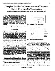
Fig. 1.

Variation in = with frequency for E

and E

1335

modes for PTFE.

The effective index method reduces to Marcatili’s method if . Fig. 1 shows the dispersion (7) is replaced with and modes for RDWG made of Teflon relation for with dimensions equal to the Ka-band (WR-28) waveguide. It can be seen that according to the Marmodes do not appear in the RDWG over catili’s method, the the Ka-band frequency range. However, when using the effecmode is tive index method, the cutoff frequency for the approximately 37 GHz. The latter is used as the condition for propagation in RDWG. single-mode B. Calculation of Dielectric Constant and Loss Tangent The calculation of the dielectric constant from effective refractive index measurements using -parameter data has been detailed in [6]–[8] where the effective complex permittivity was calculated using the Nicholson–Ross and Weir Method [12], [13]; i.e. (8) where is the complex transmission coefficient obtained from -parameter measurement data. This method is designated the NRW method to avoid confusion with the optimization method used in the later sections. It is assumed that the sample has a homogeneous material composition and is nonmagnetic, linear and isotropic. Further, we assumed that only the single mode propagates in the RDWG and the sample. The effective complex refractive index of the sample is defined as (9) where (10) (11) and , respectively, representing the real and imagwith inary parts of the effective complex permittivity. The true dielectric constant can be recovered iteratively from the effec-

tive refractive index by using the effective index method or any solution to the wave equation. Conversely, the effective for given values of index method can be used to calculate the cross section of a sample and , at a specified frequency. Therefore, a more accurate way to determine the true dielectric constant is by means of an optimization procedure, from which the loss factor (and hence, the loss tangent) and accurate sample thickness can be determined by using a suitable objective function. Our effective index model [6]–[8] allows the reflection and transmission coefficients to be expressed in simpler forms compared to other solutions to the discontinuity problem in an open dielectric waveguide, i.e. (12) (13) The following objective function was found to be the most efficient to determine , , and for 201 frequency points

(14) and are the magnitude and principal value of the where phase angle (in radians) of the transmission coefficient, and the subscripts and denote the measured and calculated values, respectively. It can be recognized immediately from (14) that the first square difference component is related to the attenuation, while the second component is associated with the phase angle of the probing wave. Therefore, it is most appropriate to in the calculation of to justify the lossless asset sumption when using the (1)–(7). The problem of multiple solutions for , , and can be reduced by applying constraints on these three parameters to stay within the desired tolerance level. Rosenbrock’s method of rotating coordinates [17], [18] was chosen to minimize the objective function (14). The method has the advantage of not requiring the evaluation of partial derivatives with respect to , , and . The method requires initial starting points that satisfy the constraints and do not lie in the boundary zones. These points are , , and with obtained chosen from the inversion method, and the initial values of

1336

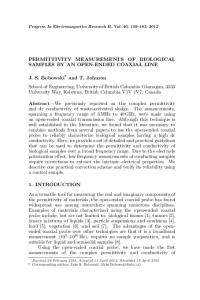
Fig. 2.


RDWG measurement setup.

in the range of 0–1. The estimated thickness was measured with a digital caliper. A computer program based on [18] was used to calculate the objective function. The iteration process is stopped when either the error function (i.e., the difference beor the iteration tween the new and previous ) is less than 10 loop count is over 10 000.

III. EXPERIMENT Fig. 2 illustrates the measurement setup using the RDWG combined transmission–reflection method. The RDWG and its one-quarter wavelength spacer (line standard for TRL calibration) have cross-sectional dimensions equal to the WR-28 standard waveguide dimension to a close tolerance of 10 m. PTFE was chosen as the RDWG material because of its ease of fabrication, very low loss and low dielectric constant. The low dielectric constant of PTFE provides a wide coverage of single-mode propagation in the RDWG at Ka-band. On the other hand, the low loss factor is an important criterion for direct application of the effective index method that assumes lossless material. The length of the RDWG beyond the horn aperture was chosen such that the surface wave has a phase shift of rad more . This length was than an ordinary endfire source [7], [19]. The RDWG was tapered only at approximately the feed section to reduce the reflection coefficient between the RDWG and the standard WR-28 waveguide. Only the -plane of the RDWG was tapered to allow a natural transition from , i.e., from center-loaded, partially the LSE mode to the dielectric-filled to completely dielectric-filled waveguide. The minimum taper length was obtained by an approximate calculation using Hecken’s method [20]. For PTFE material, the minimum taper length was approximately 36 mm long to obtain a return loss not lower than 40 dB (i.e., the reflection coefficient should not be greater than 0.01) when using the WR-28 waveguide. In this paper, the taper length was set to 40 mm. An extra 2 cm length of PTFE is further allocated within the waveguide to form a tight fit to the metal walls as well as providing support to the suspended RDWG at the waveguide opening. The length of the RDWG within the horn section is determined by the horn length. A metal waveguide horn was employed to launch the mode into the RDWG, as well as serving as a mechanical support. According to [21], the maximum launching efficiency can be achieved if the horn gradually flares out from the throat but curves back to a smaller flare angle at the mouth. In general,

it is proposed that the transverse dimension of the mouth of the horn should correspond to the inverse of the transverse propagation constants in the and directions, i.e., and at the lowest operating frequency where field extension is widest. For easy fabrication, the dimensions of the mouth were chosen as 10.5 mm 7.6 mm, and the length of the horn was 25.9 mm. All the samples used in this paper were machined from commercial planar sheets in the transverse dimension only, to a close tolerance of 10 m, while the thicknesses were left undisturbed. The thicknesses of the samples were measured using a digital caliper. All calibrations and measurements were made using the HP8510C Network Analyzer in stepped CW mode. The two-port calibration was performed for 201 frequency points in the Ka-band by employing the TRL method [9], [10]; and the details of its application to the RDWG technique have been presented elsewhere [6]–[8].

IV. RESULTS Our previous results [8] suggest increased accuracy in determination of can be obtained by using thick samples. The samples used in this work were PTFE (unsintered), polystyrene and nylon. All the samples were obtained from Polypenco Engineering Plastics Ltd., U.K. The profile of for the PTFE sample with 50 mm 50 mm cross section and measured thickness of 6.86 mm is shown in Fig. 3 together with the polynomial curve fitting line. Also, Fig. 3 shows the effect of sample thickness on if the actual thickness is between 6.7 mm and 6.9 mm, which could result in an uncertainty as high as 7% in if the measured are thickness was assumed to be accurate. The profiles of not shown as they overlapped (when using similar thicknesses used in Fig. 3), indicating a requirement for a tight tolerance in the sample thickness. The above argument suggests that the sample thickness is the most sensitive parameter to be optimized, followed by and , respectively. All step sizes for , , and were set to 10 . As a note, a single optimization run takes about 5 min to converge to the final values of , , and when using a Pentium II processor. Our selection of the optimum values of and is based on the calculated value of sample thickness which is closest to the measured values with minimum . We do not include the variation in the sample cross section, i.e., the dimensions and , as they have negligible effects on the final values of , , and provided the tolerances of both and


Fig. 3.

Variation in the dielectric constant " of a PTFE sample (50 mm

1337

2 50 mm) with frequency for an unknown thickness in a range of 6.7 mm–6.89 mm.

are kept within 0.5 mm. Furthermore, variation of and increases not only the processing time, but also the number of alternative minima. Several sets of starting values were used to account for the unimodality assumption used in the optimization procedure to obtain the possible solutions for , , and . The measured thickness (6.86 mm) was used as the initial thickness estimate for both sets, within an allowed range from 6.7 mm to 6.9 mm. The initial estimate for for the first set was 1.91, increased by 0.01 in the following sets up to 2.09. The lower and upper bounds limits of were set to 1.9 and 2.1, respectively. The opand then timization program was run twice, first with but each was allowed to vary between 0 and 1. It was , can found that the optimum values of , , and hence be obtained when the calculated thickness is 6.835 mm (representing only 0.025 mm deviation from the measured thickness) , , and . On the other with can be found for a hand, a lower objective value calculated thickness of 6.718 mm, giving a similar value but . However, the deviation from the measured with thickness was 0.142 mm, which is unusually high when using a digital caliper. Several sets of data were processed with different values of and to search for alternative solutions. However, the results indicate that lower objective values can be obtained only at the expense of higher deviation between the calculated and measured thicknesses. Comparisons between the optimization method mm and the NRW method mm for both and are shown in Fig. 4(a). Also, Fig. 5(a) compares and , which in both the real and imaginary parts of represents turn, were used to produce Fig. 6(a), where the apparent power loss obtained from the relationship: . It can be clearly seen that the -NRW in Fig. 4(a) closely follows the profile profile of in Fig. 6(a). The high was the of , which explains the main cause of the lower values of -NRW given that PTFE is a unexpectedly high values of low-loss material. The permittivity model assumes single-mode propagation in a low loss medium, and the measured power can be attributed to scattering of some of the loss energy to other higher order modes. This is taken into account

by (14) that minimizes the power loss to remove its effect on both and , as shown in Fig. 4(a). The second sample was polystyrene with a measured thickmm and ness of 4.92 mm and a cross section with mm. The measured thickness of 4.92 mm was chosen as the estimated thickness within 0.03 mm tolerance. The values of were allowed to vary in the range of 2.4–2.65 while between 0 and 1. The initial value of was chosen to be 0.9. Unwhich coincides fortunately, all sets converge to with the lower boundary of the sample thickness, i.e., 4.89 mm. can be found by seHowever, a good solution with lecting the calculated thickness of 4.915 mm, as it differs by only 0.005 mm from the measured thickness. In this case, the deviaagrees to at least the third tion in is less than 1%, and decimal digit when compared to the final objective values for a thickness of 4.89 mm. Fig. 4(b) shows good agreement in bemm and the NRW tween the optimization method mm especially below 36 GHz. As expected, method values of the NRW method show a large deviation from the those obtained using the optimization method, in spite of only a 0.005 mm difference between the measured and calculated thickness. This large deviation could not be directly interpreted just by comparing the measured and optimized -parameters shown in Fig. 5(b) but can be explained easily by Fig. 6(b) which suggests and . a large deviation between A nylon sample (which is known to be a medium-loss material) was selected to demonstrate the application of (14) even when using the lossless assumption. The measured thickness of the sample was 13.31 mm, and its cross section was 50 mm 50 mm. Various sets of data were used to find the optimum values of in the limit between 2.9 and 3.1 and between 0 and 1. Some of the results are listed in Table I. As before, the basis for selecting the optimum values of and is on the calculated thickness which is closest to the measured value. In this case, the thickness was 13.308 mm, which was only 0.002 mm different from the measured value, when and yet does not show any substantial deviation in compared to results obtained by other possible thicknesses. is quite large if the choice of opHowever, the variation in was based solely upon the smallest timum values for and value of the objective function that coincides with a calcu-

1338


(a)

(b)

(c) Fig. 4. Dielectric constant and loss tangent for (a) PTFE, (b) polystyrene, and (c) nylon samples in the Ka-band by using NRW method and optimization solution.

lated thickness of 13.289 mm. The importance of accurate measurement of the sample thickness is especially obvious if the measured thickness was 13.30 mm (instead of 13.31 mm), where a lower objective value can be obtained by choosing a calculated thickness of 13.296 mm. Fig. 4(c) compares the rebetween the optimization sults obtained for both and

method mm and NRW method mm . The effects of the deviation between the measured and calculated -parameter data shown in Fig. 5(c) are displayed in due to material absorption Fig. 6(c). The calculated is much larger than those found in the PTFE and polystyrene profiles.


1339

(a)

(b)

(c) Fig. 5.

Comparison between measured and predicted values of the real and imaginary parts of S

Further comparisons between Fig. 4(a), (b), and (c) suggest that the profiles obtained from the NRW method for all the

and S

for (a) PTFE, (b) polystyrene, and (c) nylon.

samples tend to flatten beyond 36 GHz which is close to the mode of the RDWG. Similar results were obtained from

1340


(a)

(b)

(c) Fig. 6.

Comparison between measured and predicted values of jS

j

, jS

j

other samples but with small peaks near 38.5 GHz that was slightly higher than predicted by the effective index theory. Finally, Table II provides a listing of the values of and

, and P

for (a) PTFE, (b) polystyrene, and (c) nylon.

obtained by the NRW method, optimization method, and published data assuming that the samples were from the same manufacturer. The optimization method shows good agreement in


1341

TABLE I OPTIMIZATION RESULTS FOR NYLON WITH MEASURED THICKNESS EQUAL TO 13.31 mm IN ESTIMATED " RANGE BETWEEN 2.9 AND 3.1

TABLE II COMPARISON BETWEEN NRW, OPTIMIZATION, AND OTHER TECHNIQUES

both and with the published data while the NRW method agrees reasonably only with the values. V. CONCLUSIONS We have demonstrated the use of an optimization method for RDWG dielectric measurements at the Ka-band. The technique is nondestructive, quick, and simple. Good results are obtained for the complex permittivity of a range of materials, and the issues of sensitivity and measurement errors related to sample thickness have been addressed. ACKNOWLEDGMENT The authors wish to thank J. Shipman, N. Banting, and R. Hawkes for assistance in the construction of the dielectric waveguides. REFERENCES [1] M. N. Afsar, J. R. Birch, and R. N. Clarke, “The measurement of the properties of materials,” Proc. IEEE, vol. 74, pp. 183–199, Jan. 1986. [2] J. Musil and F. Zacek, Microwave Measurements of Complex Permittivity by Free Space Methods and Their Applications. Amsterdam, The Netherlands: Elsevier, 1986.

[3] J. R. Birch et al., “An intercomparison of measurement techniques for the determination of the dielectric properties of solids at near millimeter wavelengths,” IEEE Trans. Microwave Theory Tech., vol. 42, pp. 956–965, June 1994. [4] D. K. Ghodgaonkar, V. V. Varadan, and V. K. Varadan, “A free space method for measurement of dielectric constants and loss tangents at microwave frequencies,” IEEE Trans. Instrum. Meas., vol. 38, pp. 789–793, June 1989. [5] F. C. Smith, B. Chambers, and J. C. Benett, “Methodology for accurate free-space characterization of radar absorbing materials,” Proc. Inst. Elect. Eng., Sci. Meas. Technol., vol. 141, no. 6, pp. 538–546, 1994. [6] Z. Abbas, R. D. Pollard, and R. W. Kelsall, “Further extensions to rectangular dielectric waveguide technique for dielectric measurements,” in Proc. IEEE IMTC, vol. 1, Ottawa, ON, Canada, May 19–21, 1997, pp. 44–46. , “Determination of the dielectric constant of samples from effec[7] tive refractive index measurements,” IEEE Trans. Instrum. Meas., vol. 47, pp. 148–152, Feb. 1998. [8] , “A rectangular dielectric waveguide technique for determination of permittivity of materials at W-band,” IEEE Trans. Microwave Theory Tech., vol. 46, pp. 2011–2015, Nov. 1998. [9] G. F. Engen and C. A. Hoer, “Thru-reflect-line: an improved technique for calibrating the dual 6-port automatic network analyzer,” IEEE Trans. Microwave Theory Tech., vol. MTT-27, pp. 983–987, Dec. 1979. [10] “Applying TRL Calibration to Noncoaxial Measurements,” Hewlett Packard, Product Note 8510-8a, 1988. [11] J. Musil, F. Zacek, A. Burger, and J. Karlovsky, “New microwave system to determine the complex permittivity of small dielectric and semiconducting samples,” in Proc. 4th Europ. Microwave Conf., Montreux, Switzerland, 1974, pp. 66–70.

1342


[12] A. M. Nicholson and G. F. Ross, “Measurement of the intrinsic properties of materials by time domain techniques,” IEEE Trans. Instrum. Meas., vol. IM-19, pp. 377–382, Nov. 1970. [13] W. B. Weir, “Automatic measurement of complex permittivitty and permeability at microwave frequencies,” Proc. IEEE, vol. 62, pp. 33–36, Jan. 1974. [14] S. S. Stuchly and M. Matuszewksi, “A combined total reflection-transmission method in application to dielectric spectroscopy,” IEEE Trans. Instrum. Meas., vol. IM-27, pp. 285–288, Sept.. 1978. [15] E. A. J. Marcatili, “Dielectric rectangular waveguide and directional coupler for integrated optics,” Bell Syst. Tech. J., vol. 48, pp. 2071–2102, 1969. [16] R. M. Knox and P. P. Toulios, “Intergrated circuits for millimeter through optical frequency range,” in Proc. Symp. Submillimeter Waves, New York, Mar. 1970, pp. 497–516. [17] H. H. Rosenbrock, “An automatic method for finding the greatest or least value of a function,” Comput. J., vol. 3, pp. 175–184, 1960. [18] J. L. Kuester and J. Mize, Optimization Techniques with Fortran. New York: McGraw-Hill, 1973. [19] T. N. Trinh, J. A. G. Malberbe, and R. Mittra, “A metal-to-dielectric waveguide transition with applications to millimeter-wave integrated circuits,” in IEEE MTT-S Int. Microwave Symp., 1980, pp. 205–207. [20] R. P. Hecken, “A near optimum matching section without discontinuities,” IEEE Trans. Microwave Theory Tech., vol. MTT-20, pp. 734–739, Nov. 1972. [21] W. Schlosser and H. G. Unger, “Partially filled waveguides and surface waveguides of rectangular cross section,” in Advances in Microwaves. New York: Academic, 1966, pp. 319–387. [22] R. G. Jones, “Precise dielectric measurements at 35 GHz using an open microwave resonator,” Proc. Inst. Elect. Eng., vol. 123, pp. 285–290, Apr. 1976. [23] Von Hippel, Dielectric Materials and Applications. New York: Wiley, 1954.

Zulkifly Abbas was born in Alur Setar, Malaysia, in 1962. He received the B.Sc. degree (with honors) from the University of Malaya, Serdang, Malaysia, in 1986, the M.Sc. degree from the Universiti Putra Malaysia, Serdang, in 1994, and the Ph.D. degree from the University of Leeds, Leeds, U.K., in 2000. He is currently a Lecturer in the Department of Physics, University of Malaya, where he has been a faculty member since 1987.

Roger D. Pollard (M’77–SM’91–F’97) was born in London, U.K., in 1946. He received the B.Sc. and Ph.D. degrees in electrical and electronic engineering, from the University of Leeds, Leeds, U.K. He holds the Agilent Technologies Chair in High Frequency Measurements and is Head of the School of Electronic and Electrical Engineering at the University of Leeds, where he has been a faculty member since 1974. He is an active member of the Institute of Microwaves and Photonics (one of the constituent parts of the school) which has over 40 active researchers, a strong graduate program, and has made contributions to microwave passive and active device research. The activity has significant industrial collaboration as well as a presence in continuing education. His research interests are in microwave network measurements, calibration and error correction, microwave and millimeter-wave circuits, terahertz technology, and large-signal and nonlinear characterization. He has been a Consultant to Agilent Technologies (previously Hewlett-Packard Company), Santa Rosa, CA, since 1981. He has published over 100 technical articles and three patents. Prof. Pollard is a Chartered Engineer, a Fellow of the Institution of Electrical Engineers (U.K.), and a Fellow of the IEEE “for contributions to the development of microwave and millimeter-wave measurements, and active device characterization.” He is an active IEEE volunteer, as an elected member of the Administrative Committee and 1998 President of the IEEE Microwave Theory and Techniques Society and, as Chair of the Products Committee, a member of the IEEE Technical Activities Board. He is a member of the Editorial Board of IEEE TRANSACTIONS OF MICROWAVE THEORY AND TECHNIQUES and has been on the Technical Program Committee for the IEEE MTT-S International Microwave Symposium since 1986. He also edits the book series on RF & Microwave Technology, (Piscataway, NJ: IEEE Press).

Robert W. Kelsall was born in Rotherham, U.K., in 1964. He received the B.Sc. (with honors) and Ph.D. degrees from the University of Durham, Durham, U.K., in 1985 and 1989, respectively. His doctoral research involved studies of electronic transport in GaAs quantum wells. From 1989 to 1993, he was a Research Assistant at the University of Durham and the University of Newcastle-upon-Tyne, developing Monte Carlo simulations of MOSFETs and HEMTs. In 1993, he joined the University of Leeds, Leeds, U.K., as a Lecturer in the School of Electronic and Electrical Engineering. He currently with the recently formed Institute of Microwaves and Photonics at the University of Leeds, where he is conducting research in the theory and simulation of advanced technology microwave and optoelectronic semiconductor devices. Dr. Kelsall is a member of the Institute of Physics (U.K.).