Complex systems:PC - Semantic Scholar

Product differentiation and product complexity A conceptual model and an empirical application to microcomputers

Koen Frenken Department of Innovation Studies University of Utrecht [email protected]

Paul Windrum MERIT/International Institute of Infonomics University of Maastricht [email protected]

Abstract: We propose a model of product technology that describes products as complex systems. Complex systems are made out of elements that function collectively according to the way they are put together within a system’s architecture. Different choices of elements translate into different levels of functional attributes and price. New variations in product design occur through mutations at the level of elements (“genotype”) while pre-market trials and market selection occur at the level of costs and functions (“phenotype”). In this model, both vertical and horizontal differentiation can be represented. Vertical differentiation can be understood as stemming from the use of expensive elements in high-performance product designs. Horizontal differentiation can occur when different, complementary combinations of elements yield mixes of functions each of which is preferred by a different user group. Microcomputers provide us with an interesting example of an artefact that has evolved into different varieties through a series of component innovation and recombination (Langlois and Robertson 1992). Databases on component characteristics of over 4000 different microcomputers from 1992 to 1997 are analysed on product and price differentiation using entropy statistics. Data on price allow us to distinguish between variety reflecting vertical differentiation and variety reflecting horizontal differentiation. This distinction is of importance when one wants to understand the diffusion of new component technologies through either product differentiation or price differentiation. Other issues regarding modelling and measurement of complex systems are discussed in the final section.

The authors would like to thank comments made by participants at the Eighth International Joseph A. Schumpeter Society Conference Manchester, United Kingdom, 28th June - 1st July 2000

1

1. Introduction Innovations are generally considered as successful transformations of inventions, which meet individual or collective needs. These innovations include changes in production processes, in products and services, and in organisations. While the topic of process innovation has been central in economic modelling, and the topic of organisational change in business studies, relatively few works have been focusing on product innovation. This article is about modelling and measuring product innovation. Models and measurements of product innovation are important for at least three reasons. The first reason is theoretical: process innovation and product innovation cannot always be considered as being independent. Productivity growth in production processes also stems from product innovations in capital equipment and intermediate inputs (Nelson and Winter 1977: 44). The emphasis on process innovation in economic modelling is therefore rather limited to understand the sources of productivity gains and its differences. Studies in productivity can benefit from better insight in the determinants of product innovations. The second reason is related to technology policy. A growing number of scholars argue that product innovations ultimately prevent economic systems from structural unemployment (Pasinetti 1981, 1993; Edquist et al. 1998, 2000). Targeted policies that aim at enhancing product innovation can be expected to be important to sustain long-term growth and employment. The recent emphasis on new technologies and products in industrial policies is also evidence of at least an implicit recognition of the importance of product innovation in capitalist economies. The third reason is concerned with welfare and its measurement. As product innovations lead to a growing product variety and increased product performance in products and services, these innovations contribute to welfare as more diverse needs are served at a better quality (Lancaster 1979; Windrum and Birchenhall 1998). However, qualitative change in the composition and quality of products is poorly reflected in national output statistics.1 Whereas process innovation has been modelled straightforwardly by improvements in the cost efficiency in transforming inputs into a homogeneous output, an analytical approach to product innovation requires the development of new models and concepts. We develop a system’s perspective on product development, which is derived from more general computational models of complex systems as these have been developed in evolutionary biology (Kauffman 1993; Altenberg 1997). Using this model, we can understand products as being made up by elements that interrelate in their functioning in complex ways. The important insight that is derived from an understanding of products as complex systems holds that product innovation in one part of the system creates malfunctionings in other parts of the system. The product’s working cannot solely be understood from the behaviour of its parts. The complex systems model of product development in turn informs us regarding the patterns to expect in empirical data analysis regarding the product and price differentiation in a population of product models offered on a market. The paper is organised as follows. Section 2 describes a conceptual model, which is based on Kauffman’s (1993) NK-model of complex systems and which is generalised using (1997) model of complex systems. Section 3 provides an analysis of complex patterns in variety 1

This drawback of output statistics is also emphasised in discussions on the impact of ICT on economic growth and welfare. In these debates, it is repeatedly suggested that the variety and the quality of products and services have been greatly enhanced by the introduction of ICT, but that these welfare improvements do not show up in current statistics (Solow 1987; Brynjolfsson 1993). However, as long as methodologies to measure product variety and quality are lacking, the theoretical debate remains speculative.

2

of elements used in 4444 computers introduced during the period 1992-1997 and shows how these patterns can be related to price setting in PC-market. In section 4, we briefly go into product systems that are not assembled by producers, but by consumers themselves like stereo components in hifi-systems. Section 5 list conclusions and issues for further research.

2. Product technologies as complex systems Though evolutionary economists have introduced many concepts that break with the framework of neoclassical economics, they generally follow neoclassical economists in their focus on process innovation and in their representation of technology as a coordinate in capital-labour space (Nelson and Winter 1982; Silverberg et al. 1988). In these models, technology is characterised by the required inputs to produce a particular output, and competition is solely based on relative costs-efficiency. Innovation is modelled as a stochastic, but localised process leading firms to a new coordinate in capital-labour space in the surroundings of the previous coordinate. An alternative approach to modelling innovation is based on a combinatorial logic (Kauffman 1993; Birchenhall 1995). New variations in technology can be modelled as “new combinations” between element technologies in analogy with new combinations of genes in biology. The model used here is based on the NK-model, which has been originally developed as a model of biological evolution of complex organisms (Kauffman 1988, 1993, 1995). Recently, this model has been used in simulation exercises concerning the optimisation of complex technological systems by competing agents (Kauffman et al. 1998; Auerswald et al. 2000). As for neoclassical models, these applications concerned models of process innovation, too. Here, we generalise the model to describe product innovation using Altenberg’s (1997) extension of the NK-model.

2.1 Kauffman ’s NK-model 2.1.1 Complexity Complex systems are systems containing elements that are interrelated within a particular structure (Simon 1969). The evolutionary properties of complex systems have been subject of research in theoretical biology (Monod 1971; Kauffman 1993). In biological organisms, interdependencies among genes imply a complex relation between an organism’s genotype and an organism’s phenotype. At the level of the genotype mutations occur that introduce new variants in a population. At the level of the phenotype, which is the ensemble of traits that make up an organism’s fitness, natural selection operates in terms of differential rates of reproduction. Complexity in an organism means here that a mutation in one gene may not only change the functional contribution of the mutated gene to the entire phenotype, but can also affect the functional contributions of interrelated genes to the phenotype. A gene does not simply translate into a particular trait, but operates in conjunction with other genes by regulating other genes’ state of activity. Due to these interdependencies among genes, a mutation in a single gene may have both positive effects on some traits and negative effects on other traits, which jointly determine an organism’s fitness. For this reason, the existent set of genes put structural constraints on the possible directions in further evolution: a certain phenotypic trait can only be improved by a particular mutation when the improvement in one trait outweighs the negative by-effects of this mutation with respect to other traits. In biology, this insight has led scholars to conclude that natural selection cannot be expected to lead to perfectly adapted organisms (see, e.g., Kauffman 1993: 3-26).

3

Technological systems have also been described as complex systems. For example, Simon defined technologies as man-made systems which are made up of elements that collectively attain one or a number of goals (Simon 1969 [1996]: 4; cf. Alexander 1964).2 The complexity in designing a technological system is due to the interdependence in the working of elements that make up the system. Therefore, the set of optimal choices for the elements with regard to element-specific output variables may prove sub-optimal when the effects of interdependencies between elements are taken into account. For example, tires of a car which are optimal according to tire safety tests, may not match with a particular engine which is found to be optimal in engine energy-efficiency tests, when put together in a car system. This can be due to negative effects of the particular engine type on the quality of the car as a whole when combined with particular tires, for example, caused by the vibration of the engine on the tires. There may exist an alternative type of tires that better matches with the working of the engine type as it better deals with vibration. In complex systems where elements function interdependently, the choice of element cannot be made independently from the choice of other elements due to interaction effects. Instead, the ensemble of elements has to be evaluated to analyse the overall functioning of the system design as a whole.3 The need to evaluate the working of elements at the level of the system as a whole poses a problem of complexity. Since the number of possible combinations between different variants of elements is an exponential function of the number of elements, the difficulty in finding a good system design is of a higher magnitude than finding a good element design. Simon explains combinatorial complexity of systems containing interrelated elements using the example of a working and a defective lock: “Suppose the task is to open a safe whose lock has 10 dials, each with 100 possible settings, numbered from 0 to 99. How long will it take to open the safe by a blind trial-and-error search for the correct setting? Since there are 10010 possible settings, we may expect to examine about half of these, on the average, before finding the correct one – that is, 50 billion billion settings.” (Simon 1969 [1996]: 194) The strategy of evaluating all possible combinations between elements is called global trial-anderror. Contrary to complex systems, as Simon goes on explaining, simple systems that are characterised by independency between its elements, can be optimised by local trial-and-error: “Suppose, however, that the safe is defective, so that a click can be heard when any one dial is turned to the correct setting. Now each dial can be adjusted independently and does not need to be touched again while the others are being set. The total number of settings that have to be tried is only 10 x 50, or 500. The task of opening the safe has been altered, by the cues the clicks provide, from a practically impossible one to a trivial one” (Simon 1969 [1996]: 194)

2

Hughes’ (1987: 51) concept of technological system includes, apart from technical components, organisations, scientific texts, patents, and laws. Hughes (1987: 55) does acknowledge the usefulness of approaches that define systems solely in terms of the technical components embodied. 3 This does not imply that “the whole is greater than the sum of its parts” as will become clear from the exposition of the NK-model. Confer Jervis (1997: 572) stating that “(i)f we are dealing with a system, the whole is different from not greater than the sum of its parts”.

4

In the latter case, each element can be optimised independently of the state of other elements. The problem of finding the right combination of all ten elements can be decomposed in ten subproblems, which can be solved independently. Then, the combinatorial complexity vanishes and the problem becomes feasible to handle. Simon’s example of the lock illustrates that optimisation through local trial-and-error works well for non-complex systems. In the case of complex systems, only global trial-and-error is effective in finding the optimal solution (cf. Alexander 1964 [1994]: 21). 2.1.2 The description of a complex system The anecdotal description of complexity by Simon (1969 [1996]) can be modelled analytically by Kauffman’s (1993) NK-model. This model of complex systems has been originally developed as a model of biological evolution, but its formal structure allows for applications in the domain of technological evolution through human search activity (e.g. Kauffman 1988, 1993, 1995; Kauffman and Macready 1995; Kauffman et al. 1998; Frenken et al. 1998, 1999a; Marengo 1998; Auerswald et al. 2000; Valente 2000)4 as well as applications in other domains.5 Kauffman describes a system by a string of N elements (n=1,…,N). For each element n, there exist a number of dummy values called “alleles” that refer to the possible variants of this element. The different alleles of an element are labelled by integers “0”, “1”, “2”, “3”, etc. The number of alleles of element n is described as An . For example, a particular vehicle technology can be described by the following three elements and their respective alleles: n=1 (A1=3): n=2 (A2=2): n=3 (A3=2):

an engine element with three alleles: gasoline (0), electric (1), and steam (2), a suspension element with two alleles: spring (0) and hydraulic (1), a brake element with two alleles: block (0) and disc (1).

The absence or presence of an allele in a system such as air-conditioning (yes/no) can also be coded by 0 and 1. Following the classification of elements and alleles each design can be labelled by a string of alleles. For example, following the classification above, a vehicle design with a steam engine, spring suspension and block brakes is referred to as string “200”. Each string s is described by the alleles s1s2...sN and is part of a possibility set S, for which holds: s ∈ S ; s = s1s2...sN ; sn ∈ {0,1,…,An-1}

(2.1)

The N-dimensional possibility space S is called the “design space” of a technology (Bradshaw 1992). The total number of possible strings/designs is given by the number of possible combinations between the alleles of elements. The size of the design space S is given by: S = A1 ⋅ A2 ⋅ ….. ⋅ AN

(2.2)

4

Birchenhall (1995) and Windrum and Birchenhall (1998) developed related evolutionary models of complex technological systems based on genetic algorithms. The important difference between the NKmodel and genetic algorithms is that the latter includes apart from mutation crossover as a variety generating mechanism. This mechanism holds that designs are split in two parts, which are randomly matched with parts of other designs analogous to sexual reproduction in biological evolution. The analogy in technological evolution is that particular solutions in one design can be introduced in another design and vice versa. Here, we limit the analysis to mutation as the variety generating mechanism. 5 For applications of the NK-model in organisation theory, see Kauffman (1995), Kauffman and Macready (1995), Westhoff et al. (1996), Levinthal (1997), White et al. (1997), Marengo (1998), Post and Johnson (2000).

5

In the example above, the design space adds up to 3 ⋅ 2 ⋅ 2 = 8 possible designs. The combinatorial nature of design spaces implies that its size increases exponentially for linear increases in the number of elements N. As most technological systems contain a large number of elements, the number of possible designs is generally very large with only relatively few designs being actually realised materially. The combinatorial nature of this system description requires that elements are orthogonal to one another, i.e. that elements can be treated as dimensions. Therefore, one element of a system cannot correspond with an allele of another element in the same system. For example, the description of alleles of the engine element as gasoline (0), electric (1), and steam (2) implies that the type of battery used in electric engines cannot count as another element/dimension in the description of the vehicle. The choice for a type of battery only constitutes a dimension for electric battery systems, which may or may not be an element again in a vehicle system. Put another way, the choice of battery takes place at a lower level in the decision tree: → what kind of engine ? → if electric engine: what kind of battery ? Thus, a description of a combinatorial space should therefore be such that only elements at the same level in the hierarchical decision tree are taken into account, where each element itself may again be described as a system in its own right (Hughes 1987: 55; Metcalfe 1995: 36). 2.1.3 Epistatic relations between elements The dependencies between elements in a complex system are called “ (Kauffman 1993). An epistatic relation from one element to another element implies that when the allele of the one element changes, this change affects both the functioning of the one element itself and the functioning of the element that it epistatically affects. The ensemble of epistatic relations within a technological system is called a technology’s internal structure (Simon 1969; Saviotti 1996) or, as it will be called in the following, a technology’s architecture (Henderson and Clark 1990). Imagine, for example, the architecture of a vehicle technology containing the following three epistatic relations between elements. The functionality of the engine depends only on the choice of the engine allele itself. The functionality of the suspension depends on the choice of the suspension allele itself and the engine allele. The functionality of the brake depends on the choice of the brake allele, the suspension allele and the engine allele. The architecture of these epistatic relations between the three elements can be represented as a matrix in figure 2-1 (Altenberg 1997). The x-values along the columns in the matrix indicate the vector of elements functionalities that are affected by a change in the allele of element n. The x-values along the rows indicate the vector of elements that affect the functionality of an element n. Note that x-values are always present on the diagonal (as indicated by the bold x) since the functioning of an element is by definition related to the choice of allele of this element. From this matrix, it can be derived that:

6

functionality n=1 functionality n=2 functionality n=3

n=1 n=2 n=3 ----------------------x x x x x x

Figure 2-1: Matrix representation of an architecture

-

the functionality of the first element (engine) only changes when another allele of the engine element itself is chosen the functionality of the second element (suspension) changes when another allele of the engine element and/or another when another allele of the suspension element itself is chosen the functionality of the third element (brake) changes when another allele of the engine element and/or another when another allele of the suspension and/or another allele of the brake element itself is chosen

In search for a well-working design, engineering activity can be modelled as a process of experimentation with different combinations of alleles of elements. The design space contains all these possible combinations of elements among that are open for experimentation. Search in this design space is complex since the mutation of one element also affects the working of other elements. However, it is crucial at this point to stress that the model is not restricted to this form of experimentation. Engineering can also be directed to building a new architecture in which epistatic relations between elements are reorganised, a type of innovation, which has been labeled “architectural innovation” by Henderson and Clark (1990). For example, an architecture of an automobile with the engine in the back will result in a different set of epistatic relations than an architecture with the same engine in the front. An important question thus holds which type of architectures favour search. To answer this question in this model, different architectures should be compared. The number of possible architectures increases exponentially with the number of elements that describe a system. The size of the matrix that describes a system’s architecture equals N2. For all cells except those on the diagonal, an epistatic relation can be either present or absent. The total number of possible architectures Q for a system of N elements is thus given by:

Q = 2 N ( N −1)

(2.3)

which increases exponentially for linear increases in N. Since there exist many possible architectures of complex systems, even for systems of small size, it is impracticable to analyse and compare the properties of all possible architectures of complex systems. For this reason, Kauffman (1993) restricted his analysis to particular types of architectures the property of which can be expressed in a single parameter. In his model, he used only those architectures in which each element is epistatically affected by the same number of other elements. The number of elements, by which each element is affected, is indicated by parameter K. These socalled “NK-systems” are then defined as systems with N elements in which each element is affected by K other elements. For example, the class of systems for which holds K=1 and N=3

7

refers to systems containing three elements with an architecture in which the functionality of each element depends on the allele of one other element. Importantly, though each element is affected by one element, one element may affect more or less than one other element. In this way, different architectures can be headed under the one parameter K. However, it should be borne in mind that many other architectures of epistatic relations exist that do not fall under NK-systems. For example, the architecture given in figure 2-1 does not refer to an NK-system since the elements are not affected by the same number of other elements. The engine element is not affected by any other element, the suspension element is affected by one element and the brake element is affected by two elements. 2.1.4 Search in complex fitness landscapes For systems with a given size N, the K-value can be used as a parameter to analyse the properties of systems with different degrees of complexity by means of tuning this parameter from its lowest value (K=0) to intermediate values (K=1,…, K=N-2) up to its maximum value (K=N-1). Using K as a parameter allows to compare the properties of systems with different degrees of complexity ranging from K=0 to K=N-1. Using the K-parameter, two limit cases of complexity can be distinguished. When epistatic relations are absent, we have systems of minimum complexity (K=0) and when all elements are epistatically related we have systems with maximum complexity (K=N1). Consider the example of a system consisting of three variables, N=3, each of which has two alleles, An=2. For a system with minimum complexity, all elements function independently from each other, i.e. K=0 (see figure 2-2-1). In this system the functionality of an element is solely dependent upon its own allele (here, “0” or “1”) and independent of the alleles of other variables. Following Kauffman (1993), the functional properties of this system for each design s is simulated by drawing a functionality or “fitness” value wn for each allele of each element n randomly from an uniform distribution [0,1]. The fitness of the system as a whole W is calculated as the mean value of the fitness values of elements, so we have:

W ( s) =

1 N ⋅ ∑ wn ( s n ) N n =1

(2.4)

The design space of this system contains eight strings, which can be represented as coordinates in three dimensions (a cube). Each string represents a different design with a fitness value W(s). Figure 2-2-2 presents a simulation of fitness values for K=0. The distribution of fitness values for different designs s in the design space is called a “fitness landscape”, a concept introduced by Wright (1932) in biological theory. The landscape metaphor implies that fitness values that are higher than all fitness values of neighbouring strings can be considered a “peak”. For a string that corresponds to a peak, it holds that neighbouring strings that have a different allele for one element, all have a lower fitness value. The shape of the fitness landscape structures the path of trials and error. Analogous to mutation in biology, a new design is chosen by changing the allele of one element. The value of this element changes from 0 to 1 or vice versa. A trial thus implies that one moves along one dimension in the cube from one string to a neighbouring string and on the fitness landscape from one fitness value to a neighbouring fitness value. Trial-and-error proceeds by evaluating how W is affected by this mutation. If the trial turns out to increase W, firms continue the next mutation from this string, while a lower W induces a firm to return to the previous string, and continue the next mutation from there. In a fitness landscape, local trial-and-error thus implies that as long as there exist at least one

8

neighbouring string that has a higher fitness, search will continue. Search halts when a peak string is found that can no longer be improved by means of a mutation in any one element. Search can thus be considered as an “adaptive walk” over a fitness landscape towards a “peak”, and search will only halt when a mountain peak is reached. Following the metaphor of the fitness landscape, search in complex technological systems can be considered a process of “hill-climbing” (Kauffman 1993).

w1 w2 w3

n=1 n=2 n=3 ----------------------x x x

Figure 2-2-1: Architecture of N=3-system with K=0

000: 001: 010: 011: 100: 101: 110: 111:

w1

w2

w3

W

0.2 0.2 0.2 0.2 0.7 0.7 0.7 0.7

0.6 0.6 0.9 0.9 0.6 0.6 0.9 0.9

0.8 0.5 0.8 0.5 0.8 0.5 0.8 0.5

0.53 0.43 0.63 0.53 0.70 0.60 0.80 0.70

010 (0.63) 011 (0.53)

110 (0.80) 111 (0.70)

000 (0.53)

001 (0.43)

100 (0.70)

101 (0.60)

Figure 2-2-2: Simulation of a fitness landscape of a N=3-system with K=0

Local trial-and-error in problem-solving on a fitness landscape is formally equivalent to mutation and selection in biological evolution (Simon 1969). Imagine all organisms in a population to have the same genotype described by string 000 and that a new variation is generated by a mutation in the first gene leading to 100. In the simulation, this mutation increases the organism’s fitness with from 0.53 to 0.70. As W(100) > W(000), organisms with genotype 100 will reproduce at a faster rate than organisms with genotype 000. After a sufficiently long period of selection, the population will be completely dominated by organisms that have the new string of genes 001, and the next mutation will occur in an organism with genotype 100. If the fitness of string 001 would have been lower than string 000, organisms with genotype 100 would have reproduced at a slower rate than organisms with genotype 000, and consequently, string 001 will be selected out of the population. The next mutation would then have occurred again in an organism with genotype 000.6 Consider 6

Selection in terms of genotypes’ shares in the population can be modelled using Fisher’s equation, which states that reproduction rates of genotypes are proportionate to their fitness relative to the mean (Fisher 1930).

9

now a designer that starts searching from design 000, and randomly picks the first element to be changed from 0 to 1 thus moving from 000 to 100 in the fitness landscape. Since the technology’s functionality is improved, the next mutation will start from the newly found design 100. If the fitness of design 001 would have been lower than design 000, the trial would be rejected and the next mutation would then have occurred again in design 000. The important feature of fitness landscapes of K=0 systems holds that the fitness value of an allele of an element wn (sn) is the same for all configurations of alleles of other elements. The functioning of an element is independent from the choice of allele for other elements. Therefore, the individual elements can be optimised independently through local trial-and-error. A series of random mutations in one element at the time will lead the designer to the optimum system design 110, no matter at which string a designers starts searching the fitness landscape.7 In the case of maximum complexity (K=N-1), the functioning of an allele of an element depends upon the choice of the alleles of all other elements (see, figure 2-3-1). This implies that the fitness value of a particular allele of an element is different for different configurations of alleles of other elements. To simulate the fitness landscape of this system, the fitness value of an allele of an element is randomly drawn for each possible configuration of alleles of other elements. An example of a fitness landscape of an N=K-1-system is given in figure 2-3-2. Contrary to K=0 systems, this fitness landscape contains two evolutionary optima. String 100 is a global optimum since it is the highest fitness value of all strings, while string 010 is a local optimum since fitness of this string is higher than it’s the fitness of its neighbouring strings, but lower than the fitness of the global optimum. For both global and local optima it holds that they cannot be improved by mutating a single element. The difference holds that a global optimum is the optimal solution, while local optima are sub-optimal solutions. Fitness landscapes of complex systems with epistatic relations between elements are characterised by the existence of multiple optima. In the case that several optima exist, Kauffman (1993) speaks of “rugged” fitness landscapes containing several peaks. This means that local trial-and-error search on rugged landscapes can end up in several optima. Contrary to systems with no complexity (k=0), local trial-and-error in complex systems does no longer automatically lead to the optimal solution as one runs the risk op ending up in a local optimum instead of the global optimum.8 The NK-model illustrates the general insight that a mutation in one element may improve the fitness value of some elements, but can create “technological imbalances” in other elements (Rosenberg 1969; Hughes 1987). The net result may either be a gain in fitness in which case search will continue from the newly found string, or a loss in fitness in which case search will start again from the previous string. Since, in general, several local optima exist in complex systems a designer can end up in different local optima depending on the starting point in the landscape and the particular sequence of mutations that follow. Search is “path-dependent” on the initial starting point of search and the sequence of searches that follow. By contrast, local trial-and-error in systems with no complexity (K=0) is path-independent as the global optimum is the only optimum, and any search sequence finally ends up in this optimum.9 An example of path-dependency in the simulation 7

This case corresponds to Simon’s example of a defective lock quoted in section 2.1. The solution of this defective lock can be found by evaluating the different alleles for each dial separately. Also note that in Simon’s example all strings have zero fitness in the landscape except for the solution string, which has fitness one. 8 In the context of technological evolution, this has been stressed, among others, by Alchian (1950: 219) and Simon (1969 [1996]: 46-47). 9 Path-dependency in the NK-model is different from path-dependency in models of network externalities (Arthur 1989). The term path-dependency in the NK-model refers to the path of an individual designer

10

example is when search starts from string 001 and the first mutation leads to string 000, and the second mutation to string 100. The resulting solution 100 would be optimal. However, when search starts again in 001, but the first mutation leads to 011, the next mutation will inevitably lead to the sub-optimal solution 010.10 Of course, in small design spaces, such as the eight possible designs in the example, designers can always escape local optima by simply evaluating the fitness of all eight designs. For larger systems, exhaustive search becomes very expensive since the size of the design space increases exponentially with N. Exhaustive search then becomes inefficient as the search costs no longer outweigh the marginal improvement in fitness of a global optimum over a local optimum (Frenken et al. 1998, 1999a).

w1 w2 w3

n=1 n=2 n=3 ----------------------x x x x x x x x x

Figure 2-3-1: Architecture of N=3-system with K=2

000: 001: 010: 011: 100: 101: 110: 111:

w1

w2

w3

W

0.5 0.2 0.7 0.6 0.9 0.2 0.5 0.4

0.1 0.2 0.8 0.5 0.5 0.3 0.9 0.8

0.7 0.8 0.6 0.3 0.8 0.4 0.4 0.1

0.43 0.40 0.70 0.47 0.73 0.30 0.60 0.43

010 (0.70) 011 (0.47)

110 (0.60) 111 (0.43)

000 (0.43)

001 (0.40)

100 (0.73)

101 (0.30)

Figure 2-3-2: Simulation of a fitness landscape of a N=3-system with K=2

moving within a possibility space ending up in a locally optimal string. In models of network externalities path-dependency refers to the sequence of agents adopting a technology where each new adopters increases the fitness value of a technology, which leads to a lock-in. The different terms can be distinguished by referring to microscopic path-dependency in the NK-model as it deals with an individual designer and macroscopic path-dependency as it deals with a collection of agents. 10 Design can escape the sub-optimal solution by mutating several elements at the time. In the example, the sub-optimal string 010 can be left by mutating both the first and second elements at the time. This twoelement mutation can be thought of as a jump in the fitness landscape from the sub-optimal peak to the optimal peak. Trial-and-error procedures that are not restricted to one-element mutation are discussed Frenken et al. (1999a).

11

Complex systems with rugged fitness landscapes characterise the existence of trade-offs between the functioning of different elements. Epistatic relations pose “conflicting constraints” on the optimisation of elements (Kauffman 1988, 1993, 1995). The various elements of a technology function in different degrees in different local optima. In the simulation of figure 2-3-2 optimum 100 is characterised by w1>w2 , w1>w3 , w2w3 . In this simulation, the trade-off turns out to be between optimising the functioning of the first element and third element at the expense of the second element (string 100) and optimising the second element at the expense of the first and third element (string 010).

2.2 Altenberg ’s generalised NK-model The NK-model is based on the idea that each element in a system performs an “own” subfunction within the system with regard to the attainment of one overall function on which selection operates (Kauffman 1993: 37). Each element n is conceived to have a particular fitness value wn that reflects its functional contribution to the system as a whole. The fitness of the system as a whole is derived as the average of the fitness of individual elements. In the context of technological evolution, Kauffman et al. (1998) and Auerswald et al. (2000) used the NK-model to model process technologies, or, as they call it, “production recipes”. Each recipe consists of N “operations” to produce a particular homogeneous output. For each operation n there exist An alleles that refer to a set of discrete choices for this operation. Each string then refers to a production recipe, i.e. a particular organisation of the production process. The overall fitness W of a particular string refers to the labour efficiency of a particular recipe. In these models, it is also assumed that the capital-labour ratio is constant (neutral technological progress). This specification corresponds to the model of Arrow (1962) in that the efficiency of process technologies in producing a homogeneous output is expressed in labour-efficiency. The novelty in the model concerns the existence of epistatic relations between pairs of operations, which render the labour-efficiency of an individual operation dependent on the choice of other operations. Firms can therefore not simply choose the optimal process technology as it is assumed in the original neoclassical model of the production function. Instead, they are hill-climbing the fitness landscape by experimenting with different combinations of operations through trial-anderror and run the risk of ending up in a locally optimal combination of operations. Though the NK-model fits the framework of models of process technologies, it is argued here that the application of the NK-model to an individual product technology as a car or an aircraft is limited. The NK-model is restricted to the analysis of technological systems, the fitness W of which refers to a single selection criterion (in the example above, labour-efficiency). The individual fitness values of elements wn refer to the performance of individual elements regarding their sub-function in relation to the attinment of one overall function of the system as a whole. This specification is based on the idea that each element n performs an “own” sub-function within the system, but the degree in which this function is realised wn , depends on the choice of alleles of K elements with which it is epistatically related. This system description falls short for systems that have elements that affect multiple functions of a system. For example, an epistatic effect of the vehicle’s tires on a vehicle’s engine renders the engine’s fuel-efficiency dependent on both the choice of allele of the tire element and the choice of allele of the engine element. And, an epistatic effect of a vehicle’s tires on a vehicle’s suspension renders the car’s safety dependent on both the choice of allele of the tire element and the choice of allele of the suspension element. In this example, the tire element affects two selection criteria of a car, and it cannot be said to have one “own” function.

12

A generalised model of complex systems described by N elements and F functions is needed to deal with systems that are selected on multiples functional characteristics. This model has been developed by Altenberg (1997) in the context of biology, and will be used here as a model of a complex product technology. 2.2.1 Genotype-phenotype map Altenberg (1997) developed a generalised model of complex biological organisms, which can be used to model a complex product technology. Altenberg’s generalisation of the NK-model provides a model of complex systems containing N elements (n=1,…,N) and F functions (f=1,…,F). In biological systems, for which Altenberg’s generalised NK-model was conceived, an organism’s N genes are the system’s elements and an organism’s F traits are the selection criteria. The string of genes constitutes an organism’s genotype and the set of traits constitutes an organism’s phenotype. The genotype of an organism is the level at which mutations take place that are transmitted in its offspring. The phenotype is the level at which natural selection operates in terms of its relative success to produce offspring. A single gene may affect one or several traits in the phenotype and a single trait may be affected by one or several genes in the genotype. The number of traits that is affected by a particular gene in the genotype is referred to as a gene’s 11 The number of genes that affects one particular trait in the phenotype is referred to as a traits “polygeny” (Altenberg 1997). The structure of relations between genes and traits can be represented in a “genotype-phenotype map”. This map specifies which traits are affected by which genes. An example of a genotype-phenotype map of a system with three genes (N=3) and two traits (F=2) is given in figure 2-4-1. Analogously, a technological system can be described in terms of its N elements and the F functions it performs. The string of alleles describes the “genotype” of a technological system, and the list of functional attributes describes the “phenotype” of this system. Different from process technology where fitness is expressed by a single cost criterion (process efficiency), the fitness of product technology is expressed by some weighted sum of the levels of F attributes (product quality). Typical quality attributes are speed, weight, comfort, safety, etc. Quality attributes of product technologies are generally called characteristics since Lancaster (1966) introduced this concept in economic theory. Lancaster argued that demand for a consumer technology should be understood as demand for the bundle of service characteristics that is embodied. Following Lancaster (1979: 17),“Individuals are not interested in goods for their own sake but because of the characteristics they possess”.12 Where Lancaster described product technology solely in terms of the quality attributes that are taken into account by users, Saviotti and Metcalfe (1984) proposed to describe technologies in terms of both functional attributes and technical attributes. They speak of “technical characteristics” that are subject of manipulation by designers and “service characteristics” that are the selection criteria of users.13 In our model, the technical characteristics concern the elements in 11

Matthews (1984) introduced the concept of pleiotropy in evolutionary organisation theory. The application of the concept of characteristics in economic theory has not limited to agricultural and manufactured products, but also have been applied to services (Gallouj and Weinstein 1997). 13 In the empirical framework proposed by Saviotti and Metcalfe (1984), technical characteristics and service characteristics can refer to discrete variable as well as continuous variables, while in Altenberg’s systems framework technical characteristics refer to elements with discrete choices for alleles, and service characteristics refer to continuous characteristics expressing the degree of fitness with regard to a function. 12

13

a system. These are subjects of search by designers as they experiment with different combinations of alleles in design space. Service characteristics are the “selection criteria” of a product technology that users take into account in their purchasing decision. Following this conceptualisation, an artefact can be considered as the “interface” between the designer who constructs the internal system and the user who makes use of the services it provides in particular user contexts (Simon 1969; Andersen 1991; Saviotti 1996).

• n=1

f=1

f=2

•

•

• n=2

• n=3

Figure 2-4-1: Example of a genotype-phenotype map (N=3, F=2)

Analogous to the biological model, technical characteristics make up the “genotype” of a product technology and service characteristics make up the “phenotype” of a technology. Following Altenberg (1997), the product architecture of epistatic relations between elements regarding particular functions can be represented as a genotype-phenotype map. In the example in figure 24-1, epistatic relations are such that the first and second elements are epsiatically related with regard to the first function (f=1), and the second and third elements are epistically related with reagrd to the second function (f=2). Each product architecture can now be represented by a matrix of size FxN, called the elementfunction matrix M:

M = [m fn ] , f = 1,...,F , n = 1,...,N

(2.5)

As in the NK-model, an epistatic relation is represented by x when function f is affected by element n and by – when function f is not affected by the element n. The matrix of the example in figure 2-4-1 is given in figure 2-4-2.

f=1 f=2

n=1 n=2 n=3 -----------------------x x x x

Figure 2-4-2: element-function matrix of genotype-phenotype map in figure 2-4-1

14

Each element is assumed to affect at least one function. If an element does not serve a function it is redundant in the (functional) description of the system. And, each function is assumed to be affected by at least one element. When a function is not affected by any element it is zero by definition (Altenberg 1995). Each column in the matrix M represents an element’s pleiotropy vector, which is the subset of functions that are affected by element n. The sum of x-values over a column n gives an element’s pleiotropy value, which is the number of functions affecting element n. Each row in M represents a function’s polygeny vector, which is the subset of elements that affect function f. The sum of xvalues over a row f gives the function’s polygeny value, which is the number of elements affecting function f. Division of the sum over matrix M by the number of elements N gives the system’s average pleiotropy and division of the sum over matrix M by the number of functions F gives the system’s average polygeny. In the example, the pleiotropy of the first and third element equals one and the pleiotropy of the second element equals two, and the polygeny value of both functions equals two. In total, there exist four relations between elements and functions. Average pleiotropy thus equals four-thirds and the average polygeny equals two. As explained by Altenberg (1997), an NK-system is a special case of the generalised elementfunction matrices. For NK-systems, it holds that the number of functions F equals the number of elements N. In the element-function matrix, this implies that the diagonal is always characterised by presence of a relation between element and function. Furthermore, the K-value in the NKmodel implies that each function is affected by the same number of elements. Thus, in the NKmodel the polygeny of each function is assumed to be equal to K, with pleiotropy of each element being determined randomly (with pleiotropy being on average equal to K). Dropping these two restrictions provides a general model of complex systems. 2.2.2 Fitness landscapes in the generalised NK-model The way in which fitness landscape are constructed for generalised element-function matrices follows the same logic as the original NK-model discussed in the previous section (Altenberg 1997). For each element that is mutated, all functions that are affected by this element are assigned a new, randomly drawn value from the uniform distribution [0,1]. Total fitness is again derived as the mean of the fitness values of all functions. We have:

W ( s) =

1 F ⋅ ∑ w f ( s) F f =1

(2.6)14

A simulation of the fitness landscape example of the element-function matrix given in figure 2-42 is given in figure 2-4-3 for all possible combinations between two alleles of three elements. In this simulation, a mutation in the first allele generates a random change in w1, a mutation in the second allele a random change in both w1 and w2, and a mutation in the third allele a random change in w2. Since only the second element affects both functions, the existence of local optima can only be related to different alleles of the first element (here 000 and 110). For each allele 0 or 1 of the second element, there exist an optimal set of other alleles.

14

Other specifications of the total fitness as a function of fitness values of functions in which functions are not weighted equally are discussed in the next section.

15

000: 001: 010: 011: 100: 101: 110: 111:

w1

w2

W

0.8 0.8 0.4 0.4 0.2 0.2 0.9 0.9

0.9 0.6 0.3 0.2 0.9 0.6 0.3 0.2

0.85 0.70 0.35 0.30 0.55 0.40 0.60 0.55

010 (0.35) 011 (0.30)

110 (0.60) 111 (0.55)

100 (0.55)

000 (0.85)

001 (0.70)

101 (0.40)

Figure 2-4-3: Simulation of fitness landscape of the matrix in figure 2-4-2

2.3 Function space search in a generalised selection environment The generalised NK-model of product technology includes systems with multiple service characteristics. In formula 2.6 given in the previous section, the fitness of a product technology was derived as:

W ( s) =

1 F ⋅ ∑ w f (s) F f =1

(2.7)

This formula has been specified by Altenberg (1997) to define a selection environment in order to simulate hill-climbing on a fitness landscape. The formula specifies that each function / service characteristic is weighted equally. However, as an empirical specification of quality of a product technology, this formula obviously does not account for the general case in which users may apply different weights to different service characteristics (Lancaster 1966). Generally, users do not assign the same weight to each characteristic but rank some characteristics higher than other ones. In that case, a designer can sequentially optimise service characteristics according to the ranking starting from the most preferred characteristic and ending with the less preferred service characteristic. This search strategy is called “function space search” and differs from the simple trial-and-error search rule used in NK-models and the majority of other evolutionary models. We will discuss this search strategy for homogeneous selection environments where all users apply the same ranking of service characteristics, and heterogeneous selection environments where different user groups apply different rankings of service characteristics. 2.3.1 Homogenous selection environment Allowing for different values of weights for each service characteristic that is taken into account by users, we get:

16

F

W ( s) = ∑ β f ⋅ w f ( s)

(2.8.1)

f =1

F

∑β f =1

f

= 1 , βf > 0

(2.8.2)15

A homogeneous selection environment can then be defined by some set of weights {β1, β2, … , βF} that is applied by all users of the technology. The case in which there exist heterogeneous user groups that all apply a different set of weights is discussed in section 2.3.2. The general specification of the fitness as the weighted sum of the levels of service characteristics of a design {β1, β2, … , βF} does not alter the concept of a fitness landscape as discussed in the previous section, but the number of local optima can be less .Different from the case in which all characteristics are weighted equally, local optima are more likely to be characterised by high values of the characteristics with higher weights. In the extreme case, users take only one characteristic into account. In that case, one weight equals one and all other weights equal zero. As a consequence, only the designs with the highest value for the service characteristic that is weighted by one, are (global) optima in the fitness landscape. The fitness landscapes that are constructed by the weighted sum of the values of service characteristics, can be searched in exactly the trial-and-error manner as discussed in the previous section. Importantly, in this generalised specification of the selection environment, an alternative search strategy is also possible. When service characteristics have different weights, the values of these weights can be ranked. The ranking of weights for service characteristics provide designers with information that can be used for a heuristic search strategy, heuristic meaning here a way to search the design space other than through random mutation (Simon 1969; Bradshaw 1992). Designers can sequentially optimise each function according to its ranking. This kind of search will be labelled “function space search” (Bradshaw 1992). Moreover, changes in the preferences of users can induce innovation by designers. When preferences change the ranking in service characteristics designers can be expected to direct innovation to raise the value of the service characteristic that has become more important at the cost of the characteristic that has become less important. This can be done by innovation in those elements that influence the characteristic that has become more important for users. The information of users’ ranking of weight for service characteristics allows designers to link the state of the selection environment to a research agenda. When the new ranking of weights is effectively communicated to designers, designers can change their search agenda and start mutating other elements that are known to affect the functions that has become more important. In short, through function space search, individual designers can quickly adapt to changing preferences. Put another way, variation and selection are connected through communication of preferences by users. The ranking of weights of functions act as a “focusing device” for designers 15

This is a simple function sometimes applied in multi-criteria analysis of project selection. Various alternative functions exist to choose among variants that are evaluated on multiple criteria (Nijkamp et al. 1990). An alternative specification of the total fitness function includes the possibility that the total fitness derived from the fitness level of a function is increasing, but decreasingly so, reflecting saturation (Saviotti 1998). As the model is elaborated here only as a conceptual framework, alternative functions are not discussed here.

17

as they can concentrate search efforts on those elements that are known to affect the more important functions (Rosenberg 1969). A formalised model of function space, which is presented below, goes beyond the biological metaphor of hill-climbing in models of technological evolution. Hill-climbing in design space is based on random mutations that occur independently of the state of the selection environment or changes herein. However, as argued by many students of technology studies in different ways (Rosenberg 1969; Pinch and Bijker 1984; Clark 1985; Van den Belt and Rip 1987; Henderson 1995), variation and selection in technological evolution cannot be considered as operating independently.16 Actors involved in producing new variations can be guided by the expressions of users’ preferences. Therefore, users can induce innovations directed at the improved of particular service characteristics. Function space search requires information on the matrix of the system’s architecture (which elements affect which functions), and on the selection environment (how do users weight the different functions of a technology). To identify the matrix of relations between elements and functions that make up the system’s architecture, designers first need to experiment with a number of different designs to find out the precise relations between elements and functions as contained in a product’s architecture. In the model, this can be formally expressed by mutating each element one by one and evaluating for each mutation in one element which functions are affected. This procedure would require only N mutations. A second type of information that is required for function space search concerns the values of the weights to know the ranking of service characteristics functions that users apply. This information can be collected, at least by approximation, by various means of communication with users (surveys, visits, prototype tests, etc.). Once both types of information are collected, function space search is possible. The algorithm of function space involves a sequential optimisation of the various functions by means of trial-and-error within the subset of elements that affect each function. Search starts in the subset of elements that affect the most important function, then search continues in proceeds in the subset of elements that affect the second most important function, etc. Once the most important function is optimised, the second most important function is optimised given the alleles of elements affecting the first most important function, then the third most important function is optimised given the alleles of elements affecting the first and second most important functions etc. In the example of a system containing three elements and two functions, two sequences in function space are possible: -

optimising the first function and hereafter optimising the second function given the alleles of the first and second elements which have been found optimal with regard to the first function.

-

optimising the second function and hereafter optimising the first function given the alleles of the second and third elements which have been found optimal with regard to the second function.

16

Nelson and Winter specified the selection environment as an environment “that takes the flow of innovations as given”, but they did realise that “there are important 49).

18

Following the fitness landscape in figure 4-4-3, we can now simulate function space search in a homogeneous selection environment. In the case that the first attribute is weighted higher than the second attribute (β1>β2), function space search starts with mutations in the first and second elements since only these elements affect the value w1. Since there are four possible combinations between alleles of the first and second element, four trials suffice to find the combination 11# that optimises the value for w1 (where # stands for any allele). Then, given alleles 11# for the first and second element, two trials are needed to optimise the third element with respect to w2. The optimal allele for the third element turns out to be allele 0, so search halts at 110. In the case that the second attribute is weighted higher than the first attribute (β1 W1 (110) and W2 (000) > W2 (110), since: (0.6 ⋅ 0.8) + (0.4 ⋅ 0.9) > (0.6 ⋅ 0.9) + (0.4 ⋅ 0.3), and (0.4 ⋅ 0.8) + (0.6 ⋅ 0.9) > (0.4 ⋅ 0.9) + (0.6 ⋅ 0.3) In that case, both user groups would opt for the same design 000. When heterogeneity is more dispersed, it is less likely that one design is optimal for all user groups. In the example, when the two user groups are characterised by {β11=0.9, β21 =0.1} and {β12=0.1, β22=0.9}, we have: (0.9 ⋅ 0.8) + (0.1 ⋅ 0.9) < (0.9 ⋅ 0.9) + (0.1 ⋅ 0.3), and (0.1 ⋅ 0.8) + (0.9 ⋅ 0.9) > (0.1 ⋅ 0.9) + (0.9 ⋅ 0.3) In that case, horizontal product differentiation in the Hotelling sense can also occur. In the extreme case, given a sufficiently large design space, a different design may be found for each user group with different ranking of service characteristics. When a user group exists for which no design is yet optimised, this in itself can spur innovation in particular elements in search for a new design that fits their demand. The generalised NK-model can be implemented in future simulation models. Such a model was outside the scope of the present paper, but promises an interesting way to extend simulation exercises to include product differentiation in complex products. Using this model, innovation by firms can be modelled as adaptive walks on fitness landscapes through mutation in elements. Moreover, different user groups can be represented by different fitness functions. In such models, the modelling of innovation need not be restricted to mutation in elements as in biological models. One can also allow for architectural innovations to take place that change the matrix of epistical relations between elements and functions. These simulation models can also be made relevant for product-life cycle debate in which the issue of product standardisation versus product variety is at the core (see, Saviotti 1996; Windrum and Birchenhall 1998; Frenken et al. 1999b, 2000; Frenken 2000).

17

Note that in the case of heterogeneous user groups, some weights can equal zero, while in the case of a homogeneous user group in formula 2.8.2, all weights are by definition positive. A zero weight in a homogeneous user population would imply that the feature does not count as a function for anyone.

20

In this paper, we use the model as a conceptual model to understand patterns in product differentiation in data of microcomputers. Product variety stemming from vertical and horizontal differentiation is analysed using entropy statistics. This is done by looking to what extent different price segments differentiate between different product designs as described by the alleles they incorporate. When price groups poorly differentiate between designs, different designs can be understood as having a rather similar level of functionality but for different user groups as they pay similar prices for different designs (horizontal differentiation).

3. Empirical analysis of microcomputers Using data on eight product dimensions of 4444 microcomputers, we analyse the epistatic relations over a period of six years (1992-1997). The data are taken from WHAT PC?, a leading British computer magazine on microcomputers in the United Kingdom. The list of N=8 characteristics and their An classes are given in Table 1. All variables are binary variables except for the type of processor which has twenty-two variants. The total design space thus amounts to (27) x 22 = 2816 possible PC-designs. 3.1 Dependence between elements The existence of statistical dependence between particular pairs of alleles implies that the choice of an allele of one element depends on the choice of an allele in other element as in the NKmodel and its generalised version. For example, the CD-ROM component is expected to be especially functional when it is coupled to a powerful processor (e.g., Pentium). Thus, it can be expected that a CD-ROM occurs relatively often in models with a powerful processor, while it is often absent in PC’s with low-performance processors, since users are only willing to pay for the CD-ROM component when it is coupled with powerful processors. Entropy statistics provide a straightforward methodology since it is solely based on relative frequencies in a combinatorial space (Theil 1972; Frenken et al. 1999b, 2000; Frenken 2000; cf. Langton 1990). For each pair of two elements, the alleles of the first element are labeled i (i=1,…,A1) and the alleles of the second element j (j=1,…,A2), etc. Among the eight elements that are distinguished in the dataset, there exist 1+2+3+4+5+6+7 = 28 pairs of elements (see also Appendix). For each pair of elements, the relative frequency in the total sample of product designs introduced in the same year, the relative frequency of an allele of the first element i is pi. and of an allele of the second element j is p.j. The relative joint frequency of allele i co-occurring with allele j is pij. Following Frenken et al. (1999b, 2000), variety in the choice of alleles in each element is measured by the univariate entropy, which is given by:

H (X1) = −

18

A1-1

∑{p i =0

i

⋅ log 2

( pi ) }

(3.1) 18

For 0 ⋅ log2 0 ≡ 0.

21

CPU (n=1, A1=22) 0 '8086' 1 '8088' 2 ‘8088 + 8086’ 3 ‘286’ 4 ‘386SX‘,‘386 SL’ 5 ‘386 DX’ 6 ‘486 SLC(2)’, ‘486 SL(2)’, ‘486 SLE’, ‘486 SL2’, ‘486 SXL’, ‘486‘,‘486 SX(2)’ 7 ‘486 DX’, ‘486 DX2’, ‘486 DX4’ 8 ‘Intel V25’ 9 ‘Thompson DX2’, ‘Thompson DX4‘ 10 ‘IBM BL 11 ‘586’ 12 ‘PENTIUM’ 13 ‘PENTIUMPRO’ 14 ‘IBM6x86’ 15 ‘ARN’ 16 ‘AMD’ 17 ‘Nexgen Nx586’ 18 ‘Dell Latitude’ 19 ‘V30’ 20 ‘NEC V20‘ 21 ‘Sunspark1‘, ‘Sunspark2‘ Floppy 5,25 (n=2, A1=2) 0 Absent 1 Present Floppy 3,5 (n=3, A1=2) 0 Absent 1 Present CD-ROM (n=4, A1=2) 0 Absent 1 Present Portable (n=5, A1=2) 0 No 1 Yes Colour (n=6, A1=2) 0 No 1 Yes RS232 port(s) (n=7, A1=2) 0 Absent 1 Present Harddisk (n=8, A1=2) 0 Absent 1 Present

Table 1: description of elements and alleles (N=8)

22

and the variety in the choice of combinations of alleles of two elements is given by:

∑ {p

A1-1

A2-1

i=0

j =0

H (X1 , X 2 ) = − ∑

ij

⋅ log 2

( p )}

(3.2)

ij

The mutual information between two dimensions measures the dependence between alleles of two elements, which is given by:

T (X1 , X 2 ) =

A1-1 A2-1



∑ ∑  p i =0

j =0



ij

 pij ⋅ log 2  p ⋅p  i. . j

   

(3.3)

It has been shown that (Theil 1972):

T(X1 , X2) = H(X1) – H(X2) – H(X1 , X2)

(3.4)

This relationship can be visualised as follows:

T (X1 , X2)

H(X1)

H(X2)

H (X1 , X2)

23

Mutual information measures the degree in which particular alleles of one element are coupled to particular alleles in other elements. This reflects the existence of epistatic relations as explained above in the generalised NK-model. When two elements are epistatically related, the choice of allele of one element is expected to be statistically dependent on the choice of allele of the other element, since the two elements jointly affect the functionality of one or more service characteristics.

1992

1992 - 1997 T (average) 5_6 1_5 1_8 1_6 4_5 2_3 1_3 3_8 1_4 2_5 3_6 6_8 1_2 3_5 4_6 5_8 5_7 1_7 6_7 4_8 2_4 3_7 3_4 7_8 2_6 2_7 2_8 4_7

0,1650 0,0680 0,0598 0,0548 0,0442 0,0390 0,0363 0,0316 0,0277 0,0176 0,0152 0,0150 0,0136 0,0136 0,0095 0,0093 0,0050 0,0048 0,0044 0,0035 0,0021 0,0017 0,0017 0,0012 0,0009 0,0006 0,0005 0,0004

T 2_3 1_8 1_3 1_2 1_6 6_8 3_8 1_7 2_8 2_7 3_7 6_7 3_6 2_6 7_8 1_4 1_5 2_4 2_5 3_4 3_5 4_5 4_6 4_7 4_8 5_6 5_7 5_8

0,1853 1_5 0,1361 5_6 0,0283 2_5 0,0209 1_8 0,0195 1_3 0,0075 1_6 0,0043 2_3 0,0037 1_2 0,0022 3_8 0,0019 2_4 0,0005 5_8 0,0005 6_8 0,0004 4_6 0,0003 6_7 0,0001 7_8 0,0000 1_7 0,0000 4_5 0,0000 5_7 0,0000 3_5 0,0000 3_6 0,0000 3_7 0,0000 1_4 0,0000 2_7 0,0000 2_6 0,0000 3_4 0,0000 2_8 0,0000 4_8 0,0000 4_7

1993

1994

T

T

0,1637 5_6 0,1107 1_5 0,0821 1_6 0,0723 1_8 0,0594 3_8 0,0483 1_3 0,0373 2_5 0,0369 5_7 0,0322 5_8 0,0122 6_7 0,0114 6_8 0,0095 1_2 0,0074 3_5 0,0047 1_7 0,0035 3_6 0,0029 2_3 0,0025 1_4 0,0023 2_6 0,0023 7_8 0,0020 3_7 0,0018 2_7 0,0013 2_8 0,0005 4_5 0,0003 4_6 0,0003 2_4 0,0001 3_4 0,0001 4_7 0,0001 4_8

0,2975 5_6 0,1021 1_5 0,0722 1_6 0,0636 3_5 0,0562 1_8 0,0498 1_3 0,0233 3_6 0,0185 1_4 0,0185 6_8 0,0154 4_8 0,0154 5_8 0,0148 3_8 0,0130 1_2 0,0121 1_7 0,0092 6_7 0,0073 2_3 0,0062 5_7 0,0048 3_7 0,0036 3_4 0,0024 2_4 0,0007 4_6 0,0007 4_7 0,0006 2_6 0,0003 2_7 0,0002 2_8 0,0001 7_8 0,0000 4_5 0,0000 2_5

1995 T

1996 T

0,3557 5_6 0,0527 1_4 0,0493 1_6 0,0352 3_8 0,0307 1_5 0,0231 3_6 0,0230 4_5 0,0172 4_6 0,0168 1_3 0,0142 1_8 0,0142 6_8 0,0124 3_5 0,0092 5_8 0,0066 3_7 0,0053 4_8 0,0039 1_7 0,0038 3_4 0,0019 5_7 0,0007 7_8 0,0004 6_7 0,0003 4_7 0,0002 1_2 0,0002 2_3 0,0001 2_4 0,0001 2_5 0,0001 2_6 0,0000 2_7 0,0000 2_8

0,1786 4_5 0,0893 1_6 0,0612 1_4 0,0534 5_6 0,0468 1_5 0,0341 1_8 0,0288 1_3 0,0277 3_8 0,0212 3_6 0,0193 6_8 0,0179 4_6 0,0165 3_5 0,0047 5_8 0,0038 3_4 0,0034 5_7 0,0027 4_8 0,0027 4_7 0,0004 1_7 0,0002 6_7 0,0001 3_7 0,0000 7_8 0,0000 1_2 0,0000 2_3 0,0000 2_4 0,0000 2_5 0,0000 2_6 0,0000 2_7 0,0000 2_8

1997 T 0,2332 0,0782 0,0523 0,0474 0,0428 0,0367 0,0362 0,0311 0,0227 0,0226 0,0211 0,0147 0,0073 0,0066 0,0049 0,0033 0,0022 0,0010 0,0001 0,0000 0,0000 0,0000 0,0000 0,0000 0,0000 0,0000 0,0000 0,0000

Table 2: results (graphic representation of results is given in the Appendix)

Table 2 list all results on the mutual information between the eight elements, both the average value for the whole period 1992-1997, and for each year separately. The results have been sorted from the highest value on top to the lowest value at the bottom of the table. Two things become immediately clear. First, only a few relations show strong dependency as evidenced by a high T-

24

value, while the majority of pairs show little dependency. Thus, the alleles of most elements are combined in various ways reflecting that for most elements conflicting constraints do not play an important role. The microcomputer can thus be considered highly modularised. Second, the Tvalues differ considerably from year to year. The latter result shows that microcomputer designs are continuously evolving with old combinations disappearing and new combinations emerging. We restrict our interpretation of results to the five pairs with highest T-values: 5_6 1_5 1_8 1_6 4_5

portable-colour processor-portable processor-harddisk processor-colour CD-ROM-portable

(average T = 0.1650) (average T = 0.0680) (average T = 0.0598) (average T = 0.0548) (average T = 0.0442)

Since the T-value is a summation of individual dependency values for each pair pij , we can understand the T-values by looking at which pairs of alleles occurred relatively frequent, i.e. which pairs have a high value for (pij log2 (pij / pi. · p.j).19 5_6: Desktop computers more often included a colour screen while portables incorporated more often a black-and-white screen. It indicates a strong design constraint in these dimensions: the flat screen incorporated in portable computers was very expensive in colour format, while colour monitor of desktop computers was relatively cheap. 1_5: The incorporation of high-performance processors in portable computers was rare as the weight and price increase for more powerful processors. Desktop computers did not face this design constraint and incorporate more often high performance processors. 1_8: High-performance processors were predominantly used in computers with harddisk, while computers without harddisk often included low-performance processor types. The reason is that the functionality of a harddisk is especially high when the processor type is powerful. Vice versa, the functionality of a powerful processor is especially high when a harddisk is included. 1_6: High-performance processors were predominantly used in computers with colour screen,

while computers without colour screen often included low-performance processor types. The reason is that the functionality of a colour screen is especially high when the processor type is powerful as colour-based software requires higher clock speed. 4_5: CD-ROM were first introduced in desktops an only later in portables. Design constraints in the design of portable computers possibly delayed its introduction as the incorporation of the CDROM forced designers to alter the architecture of portables while it could be incorporated in desktops without any problem. Note that CDROM’s also came as add-ons that could be purchased at extra costs.

3.2 Price and product differentiation In the previous analysis, we have been able to indicate among which elements in the PC-system dependence has been most strong. We use these five pairs of elements in our further analysis on horizontal and vertical differentiation. 19

See also Frenken (2000) on the interpretation of T-values.

25

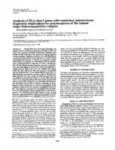
In figure 2-5, the distribution of sales prices are plotted for each year of all 4444 observations. The shapes suggest that price distributions have not changed much over the period 1992-1997 considered here (though, of course, the quality of PC’s have increased enormously over this period). We therefore classify the data in the same price segments for each year.

16000 14000 12000

Price

10000 8000 6000 4000 2000 0 0

1000 1992

2000

1993

3000

1994

1995

4000 1996

1997

Figure 2-5: Prices (in £) for 4444 PC-models introduced during the period 1992-1997

The price of each observation is classified in one out of five price segments b (b=1,…,B). The five segments are chosen such that each segment covers about the same number of observations. The segments are in £: (0-799), (800-1149), (1150-1499), (1500-1999), and (2000 and higher). The entropy of designs in each price segment b is given by:

∑ {p

A1-1 A2-1

Hb (X1 , X 2 ) = − ∑ i =0

j =0

ijb

⋅ log 2

( p )}

in bits.

26

ijb

(4.3)

The average entropy of technologies within segments weighted for their relative share, is called the weighted entropy HB and is given by (Theil 1972):

H B (X1 , X 2 ) =

B

∑{p b =1

b

⋅ Hb (X1 , X 2 ) }

(4.4)

in bits where pb stands for the relative frequency of product designs in segment b with a total number of B segments. The formula indicates to what extent each price segment is differentiating between different product designs. The two extreme cases are the following: (i)

Each segment contains only one type of design. In that case, Hb would equal zero for all b segments, and HB would equal zero too. This would indicate that price differences fully reflect functional differences between designs, which would be the case when quality is evaluated in the same way by each consumer but that different consumers prefer different qualities due to budget constraints (vertical differentiation).

(ii)

The other extreme case concerns the case in which each price segment contains as much variety in product design as the whole population of designs. In that case, HB would equal H, indicating that price to no extent differentiate between different designs. In that case, heterogeneous user groups pay the same prices for very different designs (horizontal differentiation).

It has been proven that this weighted sum of the segments’ entropy values cannot exceed the bivariate entropy of two elements (Theil 1972). The division of HB by H thus gives us a percentage that indicates to what extent variation in product design is related to horizontal differentiation. We can now relate the existence of dependence between the choice of elements as indicated by a high T-value with the degree of dependence between the choice of alleles of pairs of elements. When high T-values for a pair of elements is observed with high values for HB / H and low Tvalues with low values for HB / H, then higher dependence leads to horizontal differentiation. The choice of a particular combination between two alleles then translates into different mixes of functions with similar price each preferred by different user groups. The reverse result, when high T-values co-occur with low values for HB / H and low T-values co-occur with high values for HB / H, indicates vertical differentiation between product designs. In that case, different combinations of alleles are observed relatively often in different price segments. For the five selected pairs of elements with highest average T-value, we plotted the value for HB / H in figure 2-6-1, 2-6-2, 2-6-3, 2-6-4, and 2-6-5 The results are mixed. The 5_6 portable-colour pair and the 1_5 processor-portable pair show a (weak) positive relation with HB / H. For these three combinations, horizontal differentiation is indicated as stronger dependence tends to be observed for higher values for HB / H. 1_8 processor_harddisk pair and 1_6 processor-colour pair show no clear relationship. Finally, the 4_5 CDROM-portable shows a negative relation between mutual information and HB / H. This result indicates that the differentiation as indicated by the Tvalue between desktops with CD-ROM and portables without CD-ROM cannot be considered as evidence of horizontal product differentiation. The two combinations are generally differently priced. Examination of the data shows the desktops with CD-ROM have been sold mainly in the segments below 2000 pounds, while portables without CD-ROM mainly in the highest segment of 2000 pounds and more

27

0.95 0.93 0.91 0.89

HB / H

0.87 0.85 0.83 0.81 0.79 0.77 0.75 0.0000

0.0500

0.1000

0.1500

0.2000

0.2500

0.3000

T-value

Figure 2-6-1: Plot T-value and HB / H for element 4: “portable” and 5: “colour”

28

0.3500

0.4000

0.87 0.86 0.85

HB / H

0.84 0.83 0.82 0.81 0.80 0.79 0.78 0.0000 0.0200 0.0400 0.0600 0.0800 0.1000 0.1200 0.1400 0.1600 0.1800 T-value

Figure 2-6-2: Plot T-value and HB / H for element 1: “processor” and 5: “portable”

29

0.92 0.90

HB / H

0.88 0.86 0.84 0.82 0.80 0.78 0.0000

0.0200

0.0400

0.0600

0.0800

0.1000

0.1200

T-value

Figure 2-6-3: Plot T-value and HB / H for element 1: “processor” and 8: “

30

0.1400

0.1600

0.93 0.92 0.91 0.90

HB / H

0.89 0.88 0.87 0.86 0.85 0.84 0.83 0.0000 0.0100 0.0200 0.0300 0.0400 0.0500 0.0600 0.0700 0.0800 0.0900 T-value

Figure 2-6-4: Plot T-value and HB / H for element 1: “processor” and 6: “colour”

31

0.92

0.90

HB / H

0.88

0.86

0.84

0.82

0.80 0.0000

0.0500

0.1000

0.1500

0.2000

T-value

Figure 2-6-4: Plot T-value and HB / H for element 4: “CD-ROM” and 5: “portable”

32

0.2500

We conclude the following from these results. Horizontal differentiation is indicated for three pairs of elements in microcomputers. The user groups that come out of these results are: -

Regarding pair 5_6: users of portables with black-and-white screen and desktop users with colour screen Regarding 1_5: users of portables with low-performance processors and desktop users with high-performance processor

The combined results suggests that the global pattern of horizontal differentiation concerns portables with predominantly black-and-white screens and low-performance processors and desktops with colour screen and high-performance processors. This combined result can be readily verified by calculating the three-dimensional dependence values T (X1, X2, X3) and the three-dimensional entropy values at the level of the sample as a whole H (X1, X2, X3) and the average entropy at the level of each price segment HB (X1, X2, X3).

4. A note on systems containing independently offered products The case of microcomputers is the most common case of complex products that are offered as a package containing different alleles of elements. Likewise, several other products can be studied like transport vehicles, televisions, military equipment etc. However, there are products that are part of a system but which are independently offered by producers. For example, a CD-player can be purchased independently from other hifi equipment as interfaces between the different parts of the system are standardised.20 Similarly, the market of software contains increasingly product variants that can be combined with other products instead of being offered as a package (like Windows21). For these systems, it holds that the consumer herself combines the different alleles within a system at her will. The design activity is transferred from the producer to the consumer in that the consumer decides with combinations of alleles to use. The empirical problem that arises from this, is that data available from consumer (e-)magazines only concern alleles of individual elements of a larger system. The way consumer combine the different alleles of elements cannot be derived from this. Data gathering on systems that are combined by consumers require surveys or interviews.

5. Conclusions The generalised NK-model provides us with a conceptual model of complex products that takes into account both epistatic relations between elements affecting service characteristics and the possibility of heterogeneous user groups that value service characteristics differently. The model shows how different choices between combinations of alleles of elements translate into different mixes of service characteristics. Variety in product design can then be understood as stemming from vertical differentiation when different income groups purchase different, uniformly defined quality, and from horizontal differentiation when different user groups apply different rankings of characteristics. 20

We originally planned to include an entropy analysis of CD-players before recognising that this product is best understood as part of hifi-systems, rather than a system in its own. 21 On the Microsoft court case that is precisely about standardisation between system elements, see Windrum (1999).

33

The generalised NK-model can be implemented in future simulation models. Such a model was outside the scope of the present paper, but promises an interesting way to extend simulation exercises to include product differentiation in complex products. These simulation models can also be made relevant for product-life cycle debate in which the issue of product standardisation versus product variety is at the core (Saviotti 1996; Windrum and Birchenhall 1998; Frenken et al. 1999b, 2000). Using entropy statistics, we analyses data on alleles of elements incorporated in 4444 microcomputers introduced in the period 1992-1997 in the UK. We found that only some elements show high dependency between the choice of alleles. Further analysis on variety patterns in different price segments showed in which combinations of alleles horizontal and vertical product differentiation occurred. The general nature of the model and methodology allows for empirical analysis of many other products that can be considered complex systems. However, for complex systems that are designed by users, data can only come from survey or interviews.

34

Bibliography Alchian, A.A. (1950) ‘Uncertainty, evolution, and economic theory’, Journal of Political Economy 58, pp. 211-221. Alexander, C. (1964) Notes on the Synthesis of Form (Cambridge MA & London: Harvard University Press, 13th edition, 1994). Altenberg, L. (1997) ‘NK fitness landscapes’, section B2.7.2 in: Back, T., Fogel, D. Michalewicz, Z. (eds.) The Handbook of Evolutionary Computation (Oxford etc.: Oxford University Press). Andersen, E. (1991) ‘Techno-economic paradigms as typical interfaces between producers and consumers’, Journal of Evolutionary Economics 1, pp. 119-144. Arrow, K.J. (1962) ‘The economic implications of learning by doing’, Review of Economic Studies 29, pp. 155-173. Arthur, W.B. (1989) ‘Competing technologies, increasing returns, and lock-in by historical events’, Economic Journal 99, pp. 116-131. Auerswald P., Kauffman S., Lobo J., Shell K. (2000) ‘The production recipes approach to modeling technological innovation: an application to learning-by-doing’, Journal of Economic Dynamics And Control 24, pp. 389-450. Birchenhall, C. (1995) ‘Modular technical change and genetic algorithms’, Computational Economics 8, pp. 233-253. Bradshaw, G. (1992) ‘The airplane and the logic of invention’, pp. 239-250 in: Giere, R. (ed.) Cognitive Models of Science (Minneapolis: University of Minnesota Press). Brynjolfsson, E. (1993) ‘The productivity paradox of information technology’, Communications of the ACM 26 (12), pp. 67-77. Clark, K.B. (1985) ‘The interaction of design hierarchies and market concepts in technological Research Policy 14, pp. 235-251. Edquist, C., Hommen, L., McKelvey, M. (1998) ‘Product vs. process innovation: implications for Mitchie, J., Rerati, A. (eds.) Work, Unemployment and Need: Theory, Evidence and Policies (Cheltenham: Edward Elgar). Edquist, C., Hommen, L., McKelvey, M. (2000) Innovations and Employment in a Systems of Innovations Perspective: Process versus Product Innovations (Cheltenham: Edward Elgar). Fisher, R.A. (1930) The Genetical Theory of Natural Selection (Oxford: Clarendon Press). Frenken, K. (2000) ‘A complexity approach to innovation networks. The case of the aircraft Research Policy 29, pp. 257-272. Frenken, K., Marengo, L., Valente, M. (1998) ‘Modelling decomposition strategies in complex fitness landscapes. Implications for the economics of technical change’, Paper presented at the Seventh Conference of the International Schumpeter Society, Vienna, 13-16 June. Frenken, K., Marengo, L., Valente, M. (1999a) ‘Interdependencies, near-decomposability and adaptation’, pp. 145-165 in: Brenner, T. (ed.) Computational Techniques for Modelling Learning in Economics (Boston etc.: Kluwer).

35

Frenken, K., Saviotti, P.P., Trommetter, M. (1999b) ‘Variety and niche creation in aircraft, helicopters, motorcycles and microcomputers’, Research Policy 28, pp. 469-488. Frenken, K., Saviotti, P.P., Trommetter, M. (2000) ‘Variety and economic development: conceptual issues and measurement problems’, pp. 209-244 in: Cantner, U., Hanusch. H, Klepper, S. (eds.) Economic Evolution, Learning and Complexity (Heidelberg: PhysicaVerlag). Gallouj, F., Weinstein, O. (1997) ‘Innovation in services’, Research Policy 26, pp. 537-556. Henderson, R. (1995) ‘Of life cycles real and imaginary: The unexpectedly long old age of optical Research Policy 24, pp. 631-643. Henderson, R., Clark, K. (1990) ‘Architectural innovation’, Administrative Science Quarterly 35, pp. 9-30. Hughes, T.P. (1987) ‘The evolution of large technological systems’, pp. 51-82 in: Bijker, W. Hughes, T.P., Pinch, T.J. (eds.) The Social Construction of Technological Systems (Cambridge, Mass.: MIT Press). Jervis, R. (1997) ‘Complexity and the analysis of political and social life’, Political Science Quarterly 112, pp. 569-594. Kauffman, S.A. (1988) ‘The evolution of economic webs’, pp. 125-146 in: Anderson, P.W., Arrow, K.J., Pines, D. (eds.) The Economy as an Evolving Complex System (Redwood City CA.: Addison-Wesley). Kauffman, S.A. (1993) The Origins of Order. Self-Organization and Selection in Evolution (New York & Oxford: Oxford University Press). Kauffman, S.A. (1995) ‘Technology and evolution: escaping the Red Queen effect’, The McKinsey Quarterly (1), pp. 118-129. Kauffman, S.A., Lobo, J., Macready, W.G. (1998) ‘Optimal search on a technology landscape’, Santa Fe Working Paper 98-10-091. Kauffman, S.A., Macready, W.G. (1995) ‘Technological evolution and adaptive Complexity 1, pp. 26-43. Lancaster, K.J. (1966) ‘A new approach to consumer theory’, Journal of Political Economy 14, pp. 133-156. Lancaster, K.J. (1979) Variety, Equity and Efficiency (New York: Columbia University Press). Lancaster, K.J. (1990) ‘The economics of product variety: a survey’, Marketing Science 9, pp. 189-206. Langlois, R.N., Robertson, P.L. (1989) ‘Explaining vertical integration: lessons from the American automobile industry’, Journal of Economic History 49, pp. 361-375. Langon, C.G. (1990) ‘Computation at the edge of chaos’, Physica D, pp. 12-37. Levinthal, D. (1997) ‘Adaptation on rugged landscapes’, Management Science 43, pp. 934-950. Marengo, L. (1998) ‘Interdependencies and division of labour in problem-solving technologies’, Paper presented at the Seventh Conference of the International Schumpeter Society, Vienna, 13-16 June. Matthews, R.C.O. (1984) ‘Darwinism and economic change’, pp. 91-117 in: Collard, D.A., Dirnsdale, N.H., Gilbert, C.L., Helm, D.R., Scott, M.F.G., Sen, A.K. (eds.) Economic Theory

36

and Hicksian Themas (Oxford: Clarendon Press), reprinted pp. 159-185 in: Witt, U. (1993) (ed.) Evolutionary Economics (Aldershot: Edward Elgar). Metcalfe, J.S. (1995) ‘Technology systems and technology policy in an evolutionary framework’, Cambridge Journal of Economics 19, pp. 25-46. Monod, J. (1971) Change and Necessity (London etc.: Penguin Books). Nelson, R.R., Winter, S.G. (1977) ‘In search of useful theory of innovation’, Research Policy 6, pp. 36-76. Nelson, R.R., Winter, S.G. (1982) An Evolutionary Theory of Economic Change (Cambridge MA & London: Belknap Press of Harvard University Press). Nijkamp, P. Rietveld, P., Voogd, H. (1990) Multicriteria Evaluation and Physical Planning (Amsterdam etc.: North-Holland). Pasinetti, L.L. (1981) Structural Change and Economic Growth (Cambridge: Cambridge University Press). Pasinetti, L.L. (1993) Structural Economic Dynamics (Cambridge: Cambridge University Press). Pinch, T.J., Bijker, W.E. (1984) ‘The social construction of facts and artifacts: or how the sociology of science and the sociology of technology might benefit each other’, Social Studies of Science 14, pp. 399-442. Post, D.G., Johnson, D.R. (2000) ‘ “Chaos prevailing on every continent”: towards a new theory of decentralized decision-making in complex systems’, Chicago-Kent Law Review, forthcoming. Rosenberg, N. (1969) ‘The direction of technical change: inducement mechanisms and focussing Economic Development and Cultural Change 18, pp. 1-24, reprinted in: (1976) Perspectives on Technology (Cambridge: Cambridge University Press), pp. 108-125. Saviotti, P.P. (1996) Technological Evolution, Variety and the Economy (Cheltenham & Brookfield: Edward Elgar). Saviotti, P.P. (1998) ‘Variety and demand’, manuscript. Saviotti, P.P., Metcalfe, J.S. (1984) ‘A theoretical approach to the construction of technological Research Policy 13, pp. 141-151. Silverberg, G., Dosi, G., Orsengio, L. (1988) ‘Innovation, diversity and diffusion: a selfEconomic Journal 98, pp. 1032-1054. Simon, H.A. (1969) The Sciences of the Artificial (Cambridge MA. & London: MIT Press, 3rd edition, 1996). Solow, R.M. (1987) ‘We’d better watch out’, New York Times (July 12), p. 36. Theil, H. (1972) Statistical Decomposition Analysis (Amsterdam: North-Holland). Valente, M. (2000) Evolutionary Economics and Computer Simulations. A model for the evolution of markets. PhD thesis (Aalborg: Aalborg University), www.busines.auc.dk/~mv. Van den Belt, H., Rip, A. (1987) ‘The Nelson-Winter-Dosi model and synthetic dye chemistry’, pp. 135-158 in: Bijker, W. Hughes, T.P., Pinch, T. (eds.) The Social Construction of Technological Systems (Cambridge Mass.: MIT Press).

37

Westhoff, F.H., Yarbrough, B.V., Yarbrough, R.M. (1996) ‘Complexity, organization, and Stuart Kauffman's The Origins of Order’, Journal of Economic Behavior and Organization 29, pp. 125. White, M.C., Marin, D.B., Brazeal, D.V., Friedman, W.H. (1997) ‘The evolution of organizations: suggestions from complexity theory about the interplay between natural selection and adaptation’, Human Relations 50, pp. 1383-1401. Windrum, P. (1999) ‘Back from the brink: Microsoft and the strategic use of standards in the Paper presented at the European Meeting on Applied Evolutionary Economics, Grenoble, France, 7-9 June 1999. Windrum, P., Birchenhall, C. (1998) ‘Is product life-cycle theory a special case? Dominant designs and the emergence of market niches through coevolutionary learning’, Structural Change and Economic Dynamics 9, pp. 109-134. Wright, S. (1932) ‘The roles of mutation, inbreeding, crossbreeding, and selection in evolution’, Proceedings of the Sixth International Congress on Genetics 1, pp. 356-366.

38

APPENDIX

Graphic presentation of result on mutual information values

39

All 28 relations between the 8 elements considered

Processor type (n=1)

Harddisk y/n (n=8)

5,25 diskdrive y/n (n=2)

RS232 port y/n (n=7) (n=3)

3,5 diskdrive y/n

Colour y/n (n=6)

CD-ROM y/n (n=4)

Portable y/n (n=5)

Page A-1

40

2. Average mutual information values in the period 1992 – 1997

Processor type (n=1)

Harddisk y/n (n=8)

5,25 diskdrive y/n (n=2)

RS232 port y/n (n=7) (n=3)

3,5 diskdrive y/n

Colour y/n (n=6)

CD-ROM y/n (n=4)

Portable y/n (n=5)

= 0.250 < T < 0.100 = 0.100 < T < 0.175 = 0.175 < T < 0.250 = 0.250 < T < 0.325 = 0.325 < T < 0.400

Page A-2

41

Mutual information values for 1992

Processor type (n=1)

Harddisk y/n (n=8)

5,25 diskdrive y/n (n=2)

RS232 port y/n (n=7) (n=3)

3,5 diskdrive y/n

Colour y/n (n=6)

CD-ROM y/n (n=4)

Portable y/n (n=5)

= 0.2 < T < 0.8 = 0.8 < T < 0.14 = 0.14 < T < 0.20 = 0.20 < T < 0.26 = 0.26 < T < 0.32 = 0.32 < T < 0.38

Page A-3

42

Mutual information values for 1993

Processor type (n=1)

Harddisk y/n (n=8)

5,25 diskdrive y/n (n=2)

RS232 port y/n (n=7) (n=3)

3,5 diskdrive y/n

Colour y/n (n=6)

CD-ROM y/n (n=4)

Portable y/n (n=5)

= 0.2 < T < 0.8 = 0.8 < T < 0.14 = 0.14 < T < 0.20 = 0.20 < T < 0.26 = 0.26 < T < 0.32 = 0.32 < T < 0.38

Page A-4

43

Mutual information values for 1994

Processor type (n=1)

Harddisk y/n (n=8)

5,25 diskdrive y/n (n=2)

RS232 port y/n (n=7) (n=3)