Complexity and Infinite Games on Finite Graphs

Complexity and Infinite Games on Finite Graphs Paul William Hunter

University of Cambridge Computer Laboratory Hughes Hall July 2007

This dissertation is submitted for the degree of Doctor of Philosophy

Declaration This dissertation is the result of my own work and includes nothing which is the outcome of work done in collaboration except where specifically indicated in the text. This dissertation does not exceed the regulation length of 60 000 words, including tables and footnotes.

Complexity and Infinite Games on Finite Graphs Paul William Hunter

Summary This dissertation investigates the interplay between complexity, infinite games, and finite graphs. We present a general framework for considering two-player games on finite graphs which may have an infinite number of moves and we consider the computational complexity of important related problems. Such games are becoming increasingly important in the field of theoretical computer science, particularly as a tool for formal verification of non-terminating systems. The framework introduced enables us to simultaneously consider problems on many types of games easily, and this is demonstrated by establishing previously unknown complexity bounds on several types of games. We also present a general framework which uses infinite games to define notions of structural complexity for directed graphs. Many important graph parameters, from both a graph theoretic and algorithmic perspective, can be defined in this system. By considering natural generalizations of these games to directed graphs, we obtain a novel feature of digraph complexity: directed connectivity. We show that directed connectivity is an algorithmically important measure of complexity by showing that when it is limited, many intractable problems can be efficiently solved. Whether it is structurally an important measure is yet to be seen, however this dissertation makes a preliminary investigation in this direction. We conclude that infinite games on finite graphs play an important role in the area of complexity in theoretical computer science.

Acknowledgements A body of work this large can rarely be completed without the assistance and support of many others. Any effort to try and acknowledge all of them would undoubtedly result in one or two being left out, so I am only able to thank those that feature most prominently in my mind at the moment. The three people I am most indebted to fit nicely into the categories of my past, my present, and my future. Starting with my future (it always pays to look forwards), I am particularly grateful to Stephan Kreutzer. Working with you for a year in Berlin was a fantastic experience and I am looking forward to spending the next few years in the same city again. Thank you for all your support and guidance. To Sarah, with your constant encouragement (some would say nagging), I am forever indebted. Without your care and support I might never have finished. And I would certainly not be where or who I am today without you. Finally, the submission of this thesis ends my formal association with the person to whom I, and this dissertation, owe the most gratitude: my supervisor Anuj Dawar. Thank you for giving me the opportunity to work with you and for setting me on the path to my future. You have been an inspiration as a supervisor, I can only hope that when it is my turn to supervise PhD students I can live up to the example you have set me.

Contents 1

Introduction Notation and Conventions . . . . 1.1.1 Sets and sequences 1.1.2 Graphs . . . . . . 1.1.3 Complexity . . . . Collaborations . . . . . . . . . .

. . . . .

. . . . .

. . . . .

. . . . .

. . . . .

. . . . .

. . . . .

. . . . .

. . . . .

. . . . .

. . . . .

. . . . .

. . . . .

. . . . .

. . . . .

1 5 5 6 9 9

2 Infinite games 2.1 Preliminaries . . . . . . . . . . . . . . . . 2.1.1 Arenas . . . . . . . . . . . . . . . 2.1.2 Games . . . . . . . . . . . . . . . 2.1.3 Strategies . . . . . . . . . . . . . . 2.1.4 Simulations . . . . . . . . . . . . . 2.2 Winning condition presentations . . . . . . 2.2.1 Examples . . . . . . . . . . . . . . 2.2.2 Translations . . . . . . . . . . . . . 2.2.3 Extendibility . . . . . . . . . . . . 2.3 Complexity results . . . . . . . . . . . . . 2.3.1 P SPACE-completeness . . . . . . . 2.3.2 Complexity of union-closed games 2.4 Infinite tree automata . . . . . . . . . . . .

. . . . . . . . . . . . .

. . . . . . . . . . . . .

. . . . . . . . . . . . .

. . . . . . . . . . . . .

. . . . . . . . . . . . .

. . . . . . . . . . . . .

. . . . . . . . . . . . .

. . . . . . . . . . . . .

. . . . . . . . . . . . .

. . . . . . . . . . . . .

. . . . . . . . . . . . .

. . . . . . . . . . . . .

. . . . . . . . . . . . .

. . . . . . . . . . . . .

11 12 12 14 15 17 19 20 24 29 31 33 39 40

3 Strategy Improvement for Parity Games 3.1 The strategy improvement algorithm . . . . . . . . . . . . . . . . . . 3.2 A combinatorial perspective . . . . . . . . . . . . . . . . . . . . . . 3.3 Improving the known complexity bounds . . . . . . . . . . . . . . .

45 46 49 53

4 Complexity measures for digraphs 4.1 Tree-width . . . . . . . . . . . . . . . . . . . . 4.1.1 Structural importance of tree-width . . 4.1.2 Algorithmic importance of tree-width . 4.1.3 Extending tree-width to other structures 4.2 Directed tree-width . . . . . . . . . . . . . . . 4.3 Beyond directed tree-width . . . . . . . . . . .

57 58 60 62 62 64 66

. . . . .

. . . . .

. . . . .

. . . . .

ix

. . . . .

. . . . .

. . . . .

. . . . .

. . . . . .

. . . . . .

. . . . . .

. . . . . .

. . . . . .

. . . . . .

. . . . . .

. . . . . .

. . . . . .

. . . . . .

. . . . . .

. . . . . .

CONTENTS

x 5 Graph searching games 5.1 Definitions . . . . . . . . . . . . . . . . . . 5.1.1 Strategies . . . . . . . . . . . . . . 5.1.2 Simulations . . . . . . . . . . . . . 5.2 Examples . . . . . . . . . . . . . . . . . . 5.2.1 Cops and visible robber . . . . . . 5.2.2 Cops and invisible robber . . . . . 5.2.3 Cave searching . . . . . . . . . . . 5.2.4 Detectives and robber . . . . . . . . 5.2.5 Cops and inert robber . . . . . . . . 5.2.6 Cops and robber games . . . . . . . 5.3 Complexity measures . . . . . . . . . . . . 5.3.1 Example: Cops and visible robber . 5.3.2 Example: Cops and invisible robber 5.3.3 Example: Cops and inert robber . . 5.3.4 Example: Other resource measures 5.3.5 Monotonicity . . . . . . . . . . . . 5.4 Robustness results . . . . . . . . . . . . . . 5.4.1 Subgraphs . . . . . . . . . . . . . . 5.4.2 Connected components . . . . . . . 5.4.3 Lexicographic product . . . . . . . 5.5 Complexity results . . . . . . . . . . . . .

. . . . . . . . . . . . . . . . . . . . .

. . . . . . . . . . . . . . . . . . . . .

. . . . . . . . . . . . . . . . . . . . .

. . . . . . . . . . . . . . . . . . . . .

. . . . . . . . . . . . . . . . . . . . .

. . . . . . . . . . . . . . . . . . . . .

. . . . . . . . . . . . . . . . . . . . .

. . . . . . . . . . . . . . . . . . . . .

69 69 72 75 79 79 81 82 82 83 84 84 86 89 89 90 91 92 92 93 98 100

6 DAG-width 6.1 Cops and visible robber game . . . . . . . . . . . . . . . 6.1.1 Monotonicity . . . . . . . . . . . . . . . . . . . 6.2 DAG-decompositions and DAG-width . . . . . . . . . . 6.3 Algorithmic aspects of DAG-width . . . . . . . . . . . . 6.3.1 Computing DAG-width and decompositions . . . 6.3.2 Algorithms on graphs of bounded DAG-width . . 6.3.3 Parity Games on Graphs of Bounded DAG-Width 6.4 Relation to other graph connectivity measures . . . . . . 6.4.1 Undirected tree-width . . . . . . . . . . . . . . 6.4.2 Directed tree-width . . . . . . . . . . . . . . . . 6.4.3 Directed path-width . . . . . . . . . . . . . . .

. . . . . . . . . . .

. . . . . . . . . . .

. . . . . . . . . . .

. . . . . . . . . . .

. . . . . . . . . . .

. . . . . . . . . . .

. . . . . . . . . . .

103 104 108 109 118 118 119 120 122 123 123 124

7 Kelly-width 7.1 Games, orderings and k-DAGs . . . . . . . . . . . 7.1.1 Inert robber game . . . . . . . . . . . . . . 7.1.2 Elimination orderings . . . . . . . . . . . 7.1.3 Partial k-trees and partial k-DAGs . . . . . 7.1.4 Equivalence results . . . . . . . . . . . . . 7.2 Kelly-decompositions and Kelly-width . . . . . . . 7.3 Algorithmic aspects of Kelly-width . . . . . . . . . 7.3.1 Computing Kelly-decompositions . . . . . 7.3.2 Algorithms on graphs of small Kelly-width

. . . . . . . . .

. . . . . . . . .

. . . . . . . . .

. . . . . . . . .

. . . . . . . . .

. . . . . . . . .

. . . . . . . . .

127 128 128 130 131 132 134 137 137 140

. . . . . . . . . . . . . . . . . . . . .

. . . . . . . . . . . . . . . . . . . . .

. . . . . . . . . . . . . . . . . . . . .

. . . . . . . . . . . . . . . . . . . . .

. . . . . . . . . . . . . . . . . . . . .

. . . . . . . . .

. . . . . . . . . . . . . . . . . . . . .

. . . . . . . . .

. . . . . . . . .

CONTENTS

7.4

xi

7.3.3 Asymmetric matrix factorization . . . . . . . . . . . . . . . . Comparing Kelly-width and DAG-width . . . . . . . . . . . . . . . .

8 Havens, Brambles and Minors 8.1 Havens and brambles . . . . . . . . . . . . 8.2 Directed minors . . . . . . . . . . . . . . . 8.2.1 What makes a good minor relation? 8.2.2 Directed minor relations . . . . . . 8.2.3 Preservation results . . . . . . . . . 8.2.4 Algorithmic results . . . . . . . . . 8.2.5 Well-quasi order results . . . . . .

142 144

. . . . . . .

151 152 157 159 160 167 168 169

9 Conclusion and Future work 9.1 Summary of results . . . . . . . . . . . . . . . . . . . . . . . . . . . 9.2 Future work . . . . . . . . . . . . . . . . . . . . . . . . . . . . . . . 9.3 Conclusion . . . . . . . . . . . . . . . . . . . . . . . . . . . . . . .

171 171 173 174

References

175

. . . . . . .

. . . . . . .

. . . . . . .

. . . . . . .

. . . . . . .

. . . . . . .

. . . . . . .

. . . . . . .

. . . . . . .

. . . . . . .

. . . . . . .

. . . . . . .

. . . . . . .

xii

CONTENTS

Chapter 1

Introduction The aim of this dissertation is to investigate the interplay between infinite games, finite graphs, and complexity. In particular, we focus on two facets: the computational complexity of infinite games on finite graphs, and the use of infinite games to define the structural complexity of finite graphs. To present the motivation behind this investigation, we consider the three fundamental concepts of games, graphs and complexity.

What is a game? Ask anyone what a game is and most people will respond with an example: chess, bridge, cricket, and so on. Almost everyone understands what a game is, but few people can immediately give a precise definition. Loosely speaking, a game involves interactions between a number of players (possibly only one) with some possible outcomes, though the outcome is not always the primary concern. The importance of games in many scientific fields arises from their usefulness as an informal description of systems with complex interactions; as most people understand games, a description in terms of a game can often provide a good intuition of the system. The prevalence of this application motivates the formal study of games, which results in the use of games to provide formal definitions. Such definitions can sometimes provide interpretations of concepts where traditional approaches are cumbersome or less than adequate. For example, the semantics of Hintikka’s Independence Friendly logic [HS96] are readily expressed using games of imperfect information, but the traditional Tarski-style approaches are unwieldy. Games in computer science Mathematical games are playing an increasingly important role in computer science, both as informal descriptions and formal definitions. For example, tree-width, an algorithmically important graph parameter which we see frequently in this dissertation, can be intuitively presented as a game in which a number of cops attempt to capture a robber on a graph. Examples where games can provide formal definitions include interactive protocols and game semantics. An important example of an application of 1

2

CHAPTER 1. INTRODUCTION

games, which motivates the games we consider, is the following game that arises when verifying if a system satisfies certain requirements. Starting with the simple case of checking if a formula of propositional logic is satisfied by a truth assignment, consider the following game played by two players, Verifier and Falsifier, “on” the formula. The players recursively choose subformulas with Verifier choosing disjuncts and Falsifier choosing conjuncts until a literal is reached. If the truth value of that literal is true then Verifier wins, otherwise Falsifier wins. The formula is satisfiable if, and only if, Verifier has a strategy to always win. This game is easily extended to the verification of first order formulas, with Verifier choosing elements bounded by existential quantifiers and Falsifier choosing elements bounded by universal quantifiers. Verifying a first order logic formula is very useful for checking properties of a static system, but often in computer science we are also interested in formally verifying properties of reactive systems, systems which interact with the environment and change over time. Requirements for such systems are often specified in richer logics such as Linear Time Logic (LTL), Computation Tree Logic (CTL) or the modal µ-calculus. This motivates the following extension of the Verifier-Falsifier game for verifying if a reactive system satisfies a given set of requirements. The game is played by two players, System and Environment, on the state space of the reactive system. The current state of the system changes, either as a consequence of some move effected by Environment, or some response by System. System takes the role of Verifier, trying to keep the system in a state which satisfies the requirements to be verified. Environment endeavours to demonstrate the system does not satisfy the requirements by trying to move the system into a state which does not satisfy the requirements. The natural abstraction of these games is a game where two players move a token around a finite directed graph for a possibly infinite number of moves with the winner determined by some pre-defined condition. This abstraction encompasses many twoplayer, turn-based, zero-sum games of perfect information, and such games are found throughout computer science: in addition to the games associated with formal verification of reactive systems, examples of games which can be specified in this manner include Ehrenfeucht-Fra¨ıssé games and the cops and robber game which characterizes tree-width. Unsurprisingly, these games have been extensively researched, particularly in the area of formal verification: see for example [BL69, Mul63, EJ88, Mos91, EJ91, IK02, DJW97]. Two important questions regarding the complexity of such games are left unresolved in the literature. These are the exact complexity of deciding Muller games and the exact complexity of deciding parity games. One of the goals of this dissertation is to address these questions with an investigation of the computational complexity of deciding the winner of these types of games.

What is a graph? Graphs are some of the most important structures in discrete mathematics. Their ubiquity can be attributed to two observations. First, from a theoretical perspective, graphs are mathematically elegant. Even though a graph is a simple structure, consisting only of a set of vertices and a relation between pairs of vertices, graph theory is a rich and varied subject. This is partly due the fact that, in addition to being relational structures, graphs can also be seen as topological spaces, combinatorial objects, and many other

3 mathematical structures. This leads to the second observation regarding the importance of graphs: many concepts can be abstractly represented by graphs, making them very useful from a practical viewpoint. From an algorithmic point of view, many problems can be abstracted to problems on graphs, making the study of graph algorithms a particularly fruitful line of research. In computer science, many structures are more readily represented by directed graphs, for example: transition systems, communications networks, or the formal verification game we saw above. This means that the study of directed graphs and algorithms for directed graphs is particularly important to computer science. However, the increased descriptive power of directed graphs comes at a cost: the loss of symmetry makes the mathematical theory more intricate. In this dissertation we explore both the algorithmic and mathematical aspects of directed graphs.

What is complexity? Just as the definition of a game is difficult to pin down, the quality of “being complex” is best described by examples and synonyms. From an algorithmic perspective, a problem is more complex than another problem if the latter is easier to compute than the former. From a structural point of view, one structure is more complex than another if the first structure contains more intricacies. These are the two kinds of complexity relevant to this dissertation: computational complexity and structural complexity. In the theory of algorithms, the notion of computational complexity is well defined. In model theory however, being structurally complex is very much a subjective notion, depending largely on the application one has in mind. For example, a graph with a large number of edges could be considered more complex than a graph with fewer edges. On the other hand, a graph with a small automorphism group could be considered more complex than a graph with a large automorphism group, as the second graph (which may well have more edges) contains a lot of repetition. As we are primarily interested in algorithmic applications in this dissertation, we focus on the structural aspects of graphs which influence the difficulty of solving problems. In Section 1.1.2 below, we loosely define this notion of graph structure by describing the fundamental concepts important in such a theory. Having established what constitutes “structure”, we turn to the problem of defining structural complexity. The most natural way is to define some sort of measure which gives an intuition for how “complex” a structure is. In Chapter 4, we discuss those properties that a good measure of structural complexity should have. But how do we find such measures in the first place? Also in Chapter 4 we present the notion of treewidth and argue that it is a good measure of complexity for undirected graphs. As we remarked above, tree-width has a characterization in terms of a two-player game, so it seems that investigating similar games would yield useful measures for structural complexity. Indeed this has been an active area of research for the past few years, for example: [KP86, LaP93, ST93, DKT97, JRST01, FT03, FFN05, BDHK06, HK07]. This line of research has recently started to trend away from showing game-theoretic characterizations of established structural complexity measures to defining important parameters from the definition of the game, an example of the transition from the use of games as an informal description to their use as a formal definition. Despite this

4


activity, very little research has considered games on directed graphs. This is perhaps partly due to the lack, for some time, of a reasonable measure of structural complexity for directed graphs. The second major goal of this dissertation is to use infinite games to define a notion of structural complexity for directed graphs which is algorithmically useful.

Organization of the thesis In the remainder of this chapter we define the conventions we use throughout. Chapters 2 and 3 are primarily concerned with the analysis of the complexity of deciding the winner of infinite games on finite graphs. From Chapter 4 to Chapter 8 we investigate graph complexity measures defined by infinite games. In Chapter 2 we formally define the games we are interested in. We introduce the notion of a winning condition type and we establish a framework in which the expressiveness and succinctness of different types of winning conditions can be compared. We show that the problem of deciding the winner in Muller games is P SPACE-complete, and use this to show the non-emptiness and model-checking problems for Muller tree automata are also P SPACE-complete. In Chapter 3 we analyse an algorithm for deciding parity games, the strategy improvement algorithm of [VJ00a]. We present the algorithm from a combinatorial perspective, showing how it relates to finding a global minimum on an acyclic unique sink oriented hypercube. We combine this with results from combinatorics to improve the bounds on the running time of the algorithm. In Chapter 4 we discuss the problem of finding a reasonable notion of complexity for directed graphs. We present the definition of tree-width, arguably one of the most practical measures of complexity for undirected graphs, and we discuss the problem of extending the concept to directed graphs. Building on the games defined in Chapter 2, in Chapter 5 we define the graph searching game. We show how we can use graph searching games to define robust measures of complexity for both undirected and directed graphs. This framework is general enough to include many examples from the literature, including tree-width. In Chapters 6 and 7 we introduce two new measures of complexity for directed graphs: DAG-width and Kelly-width. Both arise from the work in Chapter 5, and both are generalizations of tree-width to directed graphs. While DAG-width is arguably the more natural generalization of the definition of tree-width, Kelly-width is equivalent to natural generalizations of other graph parameters equivalent to tree-width on undirected graphs, which we also introduce in Chapter 7. We show each measure is useful algorithmically by providing an algorithm for deciding parity games which runs in polynomial time on the class of directed graphs of bounded complexity. We compare both measures with other parameters defined in the literature such as tree-width, directed tree-width and directed path-width and show that these measures are markedly different to those already defined. Finally, in Chapter 7 we compare Kelly-width and DAG-width. We show that the two measures are closely related, but we also show that there are graphs on which the two measures differ. In Chapter 8 we present some preliminary work towards a graph structure theory for directed graphs based on DAG-width and Kelly-width. We define generalizations

5 of havens and brambles which seem to be appropriate structural features present in graphs of high complexity and absent in graphs of low complexity. We also consider the problem of generalizing the minor relation to directed graphs. We conclude the dissertation in Chapter 9 by summarizing the results presented. We discuss the contribution made towards the stated research goals, and consider directions of future research arising from this body of work.

Notation and Conventions We assume the reader is familiar with basic complexity theory, graph theory and discrete mathematics. We generally adopt the following conventions for naming objects. • For elementary objects, or objects we wish to consider elementary, for example vertices or variables: a, b, c, . . . • For sets of elementary objects: A, B, C, . . . • For structures comprising several sets, including graphs and families of sets: A, B, C, . . . • For more complex structures: A, B, C, . . . • For sequences and simple functions: α, β, γ, . . . • For more complex functions: A, B, C, . . .

1.1.1 Sets and sequences All sets and sequences we consider in this dissertation are countable. We use both N and ω to denote the natural numbers, using the latter when we require the linear order. We also assume that 0 is a natural number. Let A be a set. We denote by P(A) the set of subsets of A. For a natural number k, [A]k denotes the set of subsets of A of size k, and [A]≤k denotes the set of subsets of ˙ denotes their disjoint union and A 4 B A of size ≤ k. Given two sets A and B, A∪B denotes their symmetric difference. That is, A 4 B := (A \ B) ∪ (B \ A). For readability, we generally drop innermost parentheses or brackets when the intention is clear, particularly with functions. For example if f : P(A) → B, and a ∈ A, we write f (a) for f ({a}). We write sequences as words a1 a2 · · · , using 0 as the first index when the first element of the sequence is especially significant. For a sequence π, |π| denotes the length of π (|π| = ω if π is infinite). We denote sequence concatenation by ·. That is, if π = a1 a2 · · · an is a finite sequence and π 0 = b1 b2 · · · is a (possibly infinite) sequence, then π · π 0 is the sequence a1 a2 · · · an b1 b2 · · · . If π = a1 a2 · · · an is a finite sequence, π ω is the infinite sequence π · π · π · · · . Given a set A, the set A∗ denotes the set of all finite sequences of elements of A, and the set Aω denotes the set of all infinite


6

sequences. We say a reflexive and transitive relation ≤ on A is a well-quasi ordering if for any infinite sequence a1 a2 · · · ∈ Aω , there exists indices i < j such that xi ≤ xj . Let π = a1 a2 · · · and π 0 = b1 b2 · · · be sequences of elements of A. We write π π 0 if π is a prefix of π 0 , that is, if there exists a sequence π 00 such that π 0 = π · π 00 . We write π ≤ π 0 if π is a subsequence of π 0 , that is, there exists a sequence of natural numbers n1 < n2 < · · · such that ai = bni for all i ≤ |π|.

1.1.2 Graphs The notation we use for the graph theoretical aspects of this dissertation generally follow Diestel [Die05], however rather than regarding directed graphs as undirected graphs with two maps Head and Tail from edges to vertices, we view directed graphs as relational structures. That is, a directed graph, or digraph, G consists of a set of vertices, denoted V (G), and an edge relation, E(G) ⊆ V (G) × V (G). We use the definition in [Die05] for an undirected graph, that is E(G) is a subset of [V (G)]2 . For an edge e = (u, v) in a directed graph, the head of e is v and the tail is u, and we say e goes from u to v. To avoid ambiguities, we assume that the vertex and edge sets are disjoint. The elements of a graph G, is the set defined as Elts(G) := V (G) ∪ E(G). We note that we could either adopt the policy of Diestel and view a directed graph as an undirected graph with some additional structural information, or alternatively we could view an undirected graph as a directed graph where the edge relation is symmetric and irreflexive. We reserve those interpretations for the following two maps between directed and undirected graphs. Let D be a directed graph. The underlying undirected graph of D is the undirected graph D where: • V (D) = V (D), and • E(D) = {u, v} : (u, v) ∈ E(D)}.

← → Let G be an undirected graph. The bidirected graph of G is the directed graph G where: ← → • V ( G ) = V (G), and ← → • E( G ) = (u, v), (v, u) : {u, v} ∈ E(G)}.

We extend the definition of bidirection to parts of undirected graphs. For example a bidirected cycle is a subgraph of a directed graph which is a bidirected graph of a cycle. Regarding the pair of edges {(u, v), (v, u)} arising from bidirecting an undirected edge, we call such a pair anti-parallel. For clarity when illustrating directed graphs, we use undirected edges to represent pairs of anti-parallel edges. For the remaining definitions, we use ordered pairs to describe edges in undirected graphs. Let G be an undirected (directed) graph. A (directed) path in G is a sequence of vertices π = v1 v2 · · · such that for all i, 1 ≤ i < |π|, (vi , vi+1 ) ∈ E(G). For a subset

7 X ⊆ V (G), the set of vertices reachable from X is defined as: ReachG (X) := {w ∈ V (G) : there is a (directed) path to w from some v ∈ X}. For a subset X ⊆ V (G) of the vertices, the subgraph of G induced by X is the undirected (directed) graph G[X] defined as: • V (G[X]) = X, and • E(G[X]) = {(u, v) ∈ E(G) : u, v ∈ X}. For convenience we write G \ X for the induced subgraph G[V (G) \ X]. Similarly, for a set E of edges, G[E] is the subgraph of G with vertex set equal to the set of endpoints of E, and edge set equal to E. Let v ∈ V (D) be a vertex of a directed graph D. The successors of v are the vertices w such that (v, w) ∈ E(D). The predecessors of v are the vertices u such that (u, v) ∈ E(D). The successors and predecessors of v are the vertices adjacent to v. We say v is a root (of D) if it has no predecessors, and a leaf (of D) if it has no successors. The outgoing edges of v are all the edges from v to some successor of v, and the incoming edges of v are all the edges from a predecessor of v to v. The outdegree of v, dout (v) is the number of outgoing edges of v and the indegree of v, din (v) is the number of incoming edges of v. Given a subset V ⊆ V (G) of vertices, the out-neighbourhood of V , Nout (V ) is the set of successors of vertices of V not contained in V . If D is a directed acyclic graph (DAG), we write D for the reflexive, transitive closure of the edge relation. That is v D w if, and only if, w ∈ ReachD (v). If v D w, we say v is a ancestor of w and w is a descendant of v. We denote by Dop the directed graph obtained by reversing the directions of the edges of D. That is, Dop is the directed graph defined as: • V (Dop ) = V (D), and • E(Dop ) = (E(D))−1 = {(v, u) : (u, v) ∈ E(D)}. In this dissertation we consider transition systems with a number of transition relations. That is, a transition system is a tuple (S, sI , E1 , E2 . . .) where S is the set of states, sI ∈ S is the initial state, and Ei ⊆ S × S are the transition relations. We observe that a transition system with one transition relation is equivalent to a directed graph with an identified vertex. Structural relations As we indicated earlier, the notion of graph structure is very much a qualitative concept. Just as the “structure” of universal algebra is best characterized by subalgebras, homomorphisms and products, the particular graph structure theory we are interested in is perhaps best characterized by the following “fundamental” relations: subgraphs, connected components and graph composition. As these concepts are frequently referenced, we include their definitions. First we have the subgraph relation.


8

•

F 11

111 11

/• • G

•

•

H

•

F I *1*11

*

• **111

* ; A 1 F

1;1;**;111

1

11**;; 11

1* ;;1

• YYYYeee2/ • M;;111

Y e q

q eeeee YYYYYMYM;/, • qee • G•H

Figure 1.1: The lexicographic product of graphs G and H Definition 1.1 (Subgraph). Let G and G 0 be directed (undirected) graphs. We say G is a subgraph of G 0 if V (G) ⊆ V (G 0 ) and E(G) ⊆ E(G 0 ). The next definition describes the building blocks of a graph, the connected components. Definition 1.2 (Connected components). Let G be an undirected graph. We say G is connected if for all v, w ∈ V (G), w ∈ ReachG (v). A connected component of G is a maximal connected subgraph. It is easy to see that an undirected graph is the union of its connected components. Sm That is, if G1 ,S. . . , Gm are the connected components of G, then V (G) = i=1 V (Gi ) m and E(G) = i=1 E(Gi ). From the maximality of a connected component, it follows that a connected component is an induced subgraph. Thus we often view a connected component as a set of vertices rather than a graph. The final fundamental relation is lexicographic product, also known as graph composition. Definition 1.3 (Lexicographic product). Let G and H be directed (undirected) graphs. The lexicographic product of G and H is the directed (undirected) graph, G •H, defined as follows: • V (G • H) = V (G) × V (H), and • (v, w), (v 0 , w0 ) ∈ E(G • H) if, and only if, (v, v 0 ) ∈ E(G) or v = v 0 and (w, w0 ) ∈ E(H). Intuitively, the graph G • H arises from replacing vertices in G with copies of H, hence the name graph composition. Figure 1.1 illustrates an example of the lexicographic product of two graphs. For directed graphs we have three more basic structural concepts: weakly connected components, strongly connected components and directed union. The first two are a refinement of connected components. Definition 1.4 (Weakly/Strongly connected components). Let G be a directed graph. We say G is weakly connected if G is connected. We say G is strongly connected if for all v, w ∈ V (G), w ∈ ReachG (v) and v ∈ ReachG (w). A weakly (strongly) connected component of G is a maximal weakly (strongly) connected subgraph.

9 We observe that a directed graph is the union of its weakly connected components. The union of the strongly connected components may not include all the edges of the graph. However, it is easy to see that if there is an edge from one strongly connected component to another, then there are no edges in the reverse direction. This leads to the third structural relation specific to directed graphs. Definition 1.5 (Directed union). Let G, G1 , and G2 be directed graphs. We say G is a directed union of G1 and G2 if: • V (G) = V (G1 ) ∪ V (G2 ), and • E(G) ⊆ E(G1 ) ∪ E(G2 ) ∪ (V (G1 ) × V (G2 )). It follows that a directed graph is a directed union of its strongly connected components.

1.1.3 Complexity The computational complexity definitions of this dissertation follow [GJ79]. We consider polynomial time algorithms efficient, so we are primarily concerned with polynomial time reductions. We use standard big-O notation to describe asymptotically bounded classes of functions, particularly for describing complexity bounds.

Collaborations The work in several chapters of this dissertation arose through collaborative work with others and we conclude this introduction by acknowledging these contributions. The work regarding winning conditions in Chapter 2 was joint work with Anuj Dawar and was presented at the 30th International Symposium on Mathematical Foundations of Computer Science [HD05]. Chapter 6 arose through collaboration with Dietmar Berwanger, Anuj Dawar and Stephan Kreutzer, and was presented at the 23rd International Symposium on Theoretical Aspects of Computer Science [BDHK06]. The concept and name DAG-width were also independently developed by Jan Obdrˇza´ lek [Obd06]. Finally, the work in Chapter 7 arose through collaboration with Stephan Kreutzer and was presented at the 18th ACM-SIAM Symposium on Discrete Algorithms [HK07].

10


Chapter 2

Infinite games In this chapter we formally define the games we use throughout this dissertation. The games we are interested in are played on finite or infinite graphs (whose vertices represent a state space) with two players moving a token along the edges of the graph. The (possibly) infinite sequence of vertices that is visited constitutes a play of the game, with the winner of a play being defined by some predetermined condition. As we discussed in the previous chapter, such games are becoming increasingly important in computer science as a means for modelling reactive systems; providing essential tools for the analysis, synthesis and verification of such systems. It is known [Mar75] that under some fairly general assumptions, these games are determined. That is, for any game one player has a winning strategy. Furthermore, under the conditions we consider below, the games we consider are decidable: whichever player wins can be computed in finite time [BL69]. We are particularly interested in the computational complexity of deciding which player wins in these games. Indeed, this forms one of the underlying research themes of this dissertation. As we are interested in the algorithmic aspects of these games, we need to restrict our attention to games that can be described in a finite fashion. This does not mean that the graph on which the game is played is necessarily finite as it is possible to finitely describe an infinite graph. Nor does having a finite game graph by itself guarantee that the game can be finitely described. Even with two nodes in a graph, the number of distinct plays can be uncountable and there are more possible winning conditions than one could possibly describe. Throughout this dissertation, we are concerned with Muller games played on finite graphs. These are games in which the graph is finite and the winner of a play is determined by the set of vertices of the graph that are visited infinitely often in the play (see Section 2.1 for formal definitions). This category of games is wide enough to include most kinds of game winning conditions that are considered in the literature, including Streett, Rabin, Büchi and parity games. Since the complexity of a problem is measured as a function of the length of the description, the complexity of deciding which player wins a game depends on how exactly the game is described. In general, a Muller game is defined by a directed graph A, and a winning condition F ⊆ P(V (A)) consisting of a set of subsets of V (A). One could specify F by listing all its elements explicitly (we call this an explicit 11

12

CHAPTER 2. INFINITE GAMES

presentation) but one could also adopt a formalism which allows one to specify F more succinctly. In this chapter we investigate the role the specification of the winning condition has in determining the complexity of deciding regular games. Examples of this line of research can be found throughout the literature, for instance the complexity of deciding Rabin games is known to be NP-complete [EJ88], for Streett games it is known to be co-NP-complete. The complexity of deciding parity games is a central open question in the theory of regular games. It is known to be in NP ∩ co-NP [EJ91] and conjectured by some to be in P TIME. In Chapters 3, 6 and 7 we explore this problem in more detail. For Muller games, the exact complexity has not been fully investigated. In Section 2.3 we show that the complexity of deciding Muller games is P SPACE -complete for many types of presentation. We also establish a framework in which the expressiveness and succinctness of different types of winning conditions can be compared. We introduce a notion of polynomial time translatability between formalisms which gives rise to a notion of game complexity stronger than that implied by polynomial time reductions of the corresponding decision problems. Informally, a specification is translatable into another if the representation of a game in the first can be transformed into a representation of the same game in the second. The complexity results we establish for Muller games allow us to show two important problems related to Muller automata are also P SPACE -complete: the nonemptiness problem and the model-checking problem on regular trees. The chapter is organised as follows. In Section 2.1 we present the formal definitions of arenas, games and strategies that we use throughout the remainder of the dissertation. In Section 2.2 we introduce the notion of a winning condition type, a formalization for specifying winning conditions. We provide examples from the literature and we consider the notion of translatability between condition types. In Section 2.3 we present some results regarding the complexity of deciding the games we consider here, including the P SPACE -completeness result for Muller games, and a co-NP-completeness result for two games we introduce. Finally, in Section 2.4 we show that the non-emptiness and model checking problems for Muller tree automata are also P SPACE -complete.

2.1 Preliminaries In this section we present the definitions of arenas, games and strategies that we use throughout the dissertation. The definitions we use follow [GTW02]. In Section 2.1.4 we introduce a generalization of bisimulation appropriate for arenas and games, game simulation, and we show how it can be used to translate plays and strategies from one arena to another.

2.1.1 Arenas Our first definition is a generalization of a transition system where two entities or players control the transitions. Definition 2.1 (Arena). An arena is a tuple A := (V, V0 , V1 , E, vI ) where:

2.1. PRELIMINARIES

13 . v1

u lllll l v4 RR [ RRRR)

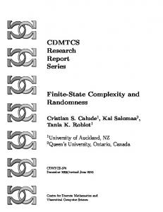
v2 iRR v RRRR ll 3 iRRRRRR ullll ) ) l5 v5 RRRRR l5 v6 l l l l l l R) ll ll v7 v8 v9 n

Figure 2.1: An example of an arena • (V, E) is a directed graph, • V0 , the set of Player 0 vertices, and V1 , the set of Player 1 vertices, form a partition of V , and • vI ∈ V is the initial vertex. Viewing arenas as directed graphs with some additional structure, we define the notions of subarena and induced subarena in the obvious way. Figure 2.1 illustrates an arena A with V0 (A) = {v4 , v5 , v6 } and V1 (A) = {v1 , v2 , v3 , v7 , v8 , v9 }. Given an arena, A, we consider the following set of interactions between two players: Player 0 and Player 1.1 A token, or pebble, is placed on vI (A). Whenever the pebble is on a vertex v ∈ V0 (A), Player 0 chooses a successor of v and moves the pebble to that vertex, and similarly when the pebble is on a vertex v ∈ V1 (A), Player 1 chooses the move. This results in a (possibly infinite) sequence of vertices visited by the pebble. We call such a sequence a play. More formally, Definition 2.2 (Play). Given an arena A and v ∈ V (A), a play in A (from v) is a (possibly infinite) sequence of vertices v1 v2 · · · such that v1 = v and for all i ≥ 1, (vi , vi+1 ) ∈ E(A). If v is not specified, we assume the play is from vI (A). The set of all plays in A from vI (A) is denoted by Plays(A). We observe that if A0 is a subarena of A then Plays(A0 ) ⊆ Plays(A). As an example, the infinite sequence v1 v4 v7 v5 v8 v6 v9 v4 v7 (v5 v2 )ω is a play in the arena pictured in Figure 2.1, as is the finite sequence v1 v4 v7 v5 v8 v6 v9 v4 . When one of the players has no choice of move, we may assume that there is only one player as there is no meaningful interaction between the players. Definition 2.3 (Single-player arena). Let A = (V, V0 , V1 , E, vI ) be an arena. We say A is a single-player arena if for some i ∈ {0, 1} and every v ∈ Vi , dout (v) ≤ 1. An important concept relating to arenas and the games we consider is the notion of duality. In the dual situation, we interchange the roles of Player 0 and Player 1. This gives us the following definition of a dual arena. 1 For

convenience we use the feminine pronoun for Player 0 and the masculine pronoun for Player 1

14


Definition 2.4 (Dual arena). Let A = (V, V0 , V1 , E, vI ) be an arena. The dual arena of A is the arena defined by Ae := (V, V1 , V0 , E, vI ). e We observe that for each arena A, Plays(A) = Plays(A).

2.1.2 Games

Arenas and plays establish the interactions that we are concerned with. We now use these to define games by imposing outcomes for plays. The games we are interested in are zero-sum games, that is, if one player wins then the other player loses. We can therefore define a winning condition as a set of plays that are winning for one player, say Player 0, working on the premise that if a play is not in that set then it is winning for Player 1. Definition 2.5 (Game). A game is a pair G := (A, Win) where A is an arena and Win ⊆ Plays(A). For π ∈ Plays(A) if π ∈ Win, we say π is winning for Player 0, otherwise π is winning for Player 1. A single-player game is a game (A, Win) where A is a single player arena. As we mentioned earlier, to consider algorithmic aspects of these games we need to assume that they can be finitely presented. Muller games are an important example of a class of finitely presentable games. With a Muller game, if a player cannot move then he or she loses, otherwise the outcome of an infinite play is dependent on the set of vertices visited infinitely often. Definition 2.6 (Muller game). A game G = (A, Win) is a Muller game if A is finite and there exists F ⊆ P(V (A)) such that for all π ∈ Plays(A): ( π is finite and ends with a vertex from V1 (A), or π ∈ Win ⇐⇒ π is infinite and {v : v occurs infinitely often in π} ∈ F. If G is a Muller game, witnessed by F ⊆ P(V (A)), we write G = (A, F ). As an example, consider the arena A pictured in Figure 2.1. Let F = {v2 , v5 } . Then G = (A, F ) is a Muller game. The play v1 v4 v7 v5 v8 v6 v9 v4 v7 (v5 v2 )ω is winning for Player 0, but the play v1 v4 v7 (v5 v8 v6 v9 v4 v7 )ω is winning for Player 1. The games used in the literature in the study of logics and automata are generally Muller games. In these games, the set F is often not explicitly given but is specified by means of a condition. Different types of condition lead to various different types of games. We explore this in more detail in Section 2.2. An important subclass of Muller games are the games where only one player wins any infinite play. Games such as Ehrenfeucht-Fra¨ıssé games (on finite structures) [EF99] and the graph searching games we consider in Chapter 5 are examples of these types of games. Definition 2.7 (Simple game). A Muller game G = (A, F ) is a simple game if either F = ∅, or F = P(V (A)).

2.1. PRELIMINARIES

15

Two other important subclasses of Muller games which we consider in this chapter are union-closed and upward-closed games. Definition 2.8 (Union-closed and Upward-closed games). A Muller game G = (A, F ) is union-closed if for all X, Y ∈ F, X ∪ Y ∈ F. G is upward-closed if for all X ∈ F and Y ⊇ X, Y ∈ F. Remark. Union-closed games are often called Streett-Rabin games in the literature, as Player 0’s winning set can be specified by a set of Streett pairs (see Definition 2.38 below) and Player 1’s winning set can be specified by a set of Rabin pairs (see Definition 2.37). However, to minimize confusion, we reserve the term Streett game for union-closed games with a condition presented as a set of Streett pairs, and the term Rabin game for the dual of a union-closed game (see below) with a condition presented as a set of Rabin pairs. We conclude this section by considering dual games and subgames. In Definition 2.4 we defined the dual of an arena. The dual game is played on the dual arena, but we have to complement the winning condition in order to fully interchange the roles of the players. That is, e := (A, e Win) Definition 2.9 (Dual game). Let G = (A, Win) be a game. The game G where Ae is the dual arena of A and Win = Plays(A) \ Win is the dual game of G.

Given a game on an arena A we can define a restricted game on a subarena A0 by restricting the winning condition to valid plays in the subarena.

Definition 2.10 (Subgame). Let G = (A, Win) be a game, and A0 a subarena of A. The subgame induced by A0 is the game G0 = (A0 , Win0 ) where Win0 = Win ∩ Plays(A0 ).

2.1.3 Strategies As with most games we are less interested in outcomes of single plays in the game and more interested in the existence of strategies that ensure one player wins against any choice of moves from the other player. Definition 2.11 (Strategy). Let A = (V, V0 , V1 , E, vI ) be an arena. A strategy (for Player i) in A is a partial function σ : V ∗ Vi → V such that if σ(v1 v2 · · · vn ) = v 0 then (vn , v 0 ) ∈ E. A play π = v1 v2 · · · is consistent with a strategy σ if for all j < |π| such that vj ∈ Vi , σ(v1 v2 · · · vj ) = vj+1 . Given a sequence of vertices visited, ending with a vertex in Vi , a strategy for Player i gives the vertex that Player i should then play to. We observe that given a strategy σ for Player 0 and a strategy τ for Player 1 from any vertex v there is a unique maximal play πτσ from v consistent with σ and τ in the sense that any play consistent with both strategies is a prefix of πτσ . We call this play the play (from v) defined by strategies σ and τ . A useful class of strategies are those that can be defined from a fixed number of previously visited vertices.

16


Definition 2.12 (Strategy memory). If a strategy σ has the property that for some fixed m, σ(w) = σ(w0 ) if w and w0 agree on their last m letters, then we say that the strategy requires finite memory (of size m − 1). If m = 1, we say the strategy is memoryless or positional. Strategies extend to games in the obvious way. Definition 2.13 (Game strategies). Given a game G = (A, Win), a strategy for Player i in G is a strategy for Player i in A. A strategy σ for Player i is winning if all plays consistent with σ are winning for Player i. Player i wins G if Player i has a winning strategy from vI (A). We observe that for any play π = v1 v2 · · · vn in a Muller game, consistent with a winning strategy σ for Player i, if vn ∈ Vi (A) then σ(π) is defined. Earlier we alluded to the following important result of Büchi and Landweber [BL69]. Theorem 2.14 ([BL69]). Let G = (A, F ) be a Muller game. One player has a winning strategy on G with finite memory of size at most |V (A)|!. An immediate corollary of this is that Muller games are decidable: we can check all possible strategies for both players that use at most |V (A)|! memory, and see if the corresponding defined plays are winning. However, the complexity bounds on such an algorithm are enormous. In [McN93] McNaughton provided an algorithm with considerably better space and time bounds. Theorem 2.15 ([McN93]). Let G = (A, F ) be a Muller game with A = (V, V0 , V1 , E, vI ). Whether Player 0 has a winning strategy from vI can be decided in time O(|V |2 |E||V |!) and space O(|V |2 ). For union-closed games and their duals we can reduce the memory requirement for a winning strategy. Theorem 2.16 ([Kla94]). Let G = (A, F ) be a Muller game. If F is closed under unions and Player 1 has a winning strategy, then Player 1 has a memoryless winning strategy. Dually, if the complement of F is closed under union and Player 0 has a winning strategy, then Player 0 has a memoryless winning strategy. Two useful tools for constructing decidability algorithms are force-sets and avoid-sets. Definition 2.17 (Force-set and Avoid-set). Let A be an arena, and X, Y ⊆ V (A). i The set ForceX (Y ) is the set of vertices from which Player i has a strategy σ such that any play consistent with σ reaches some vertex in Y without leaving X. The set i (Y ) is the set of vertices from which Player i has a strategy σ such that any AvoidX play consistent with σ that remains in X avoids all vertices in Y . 1−i i We observe from the definitions that ForceX (Y ) = X \ AvoidX (Y ). We also observe that we may assume the strategies σ are memoryless: if Player i can force the play from v to some vertex of Y , the play to v is irrelevant. Computing a force-set is an instance of the well-known alternating reachability problem, and in Algorithm 2.1 we present the standard algorithm for computing a force-set. Nerode, Remmel and Yakhnis [NRY96] provide an implementation of this algorithm which runs in time O(|E(A)|), giving us the following:

2.1. PRELIMINARIES

17

0 Lemma 2.18. Let A be an arena. For any sets X, Y ⊆ V (A), ForceX (Y ) can be computed in time O(|E(A)|)

0 Algorithm 2.1 F ORCE X (Y ) Returns: The set of vertices v ∈ V (A) such that Player 0 has a strategy to force a play from v to some element of Y without visiting a vertex outside X. let R = {v ∈ V0 (A) ∩ X : there exists w ∈ Y with (v, w) ∈ E(A)}. let S = {v ∈ V1 (A) ∩ X : for all w with (v, w) ∈ E(A), w ∈ Y }. if R ∪ S ⊆ Y then return Y else 0 return F ORCE X (R ∪ S ∪ Y ).

2.1.4 Simulations One of the most important concepts in transition systems is the notion of bisimulation. Two transition systems are bisimilar if each system can simulate the other. That is, Definition 2.19 (Bisimulation). Let T = (S, s0 , E) and T 0 = (S 0 , s00 , E 0 ) be transition systems. We say T and T 0 are bisimilar if there exists a relation ∼⊆ S × S 0 such that: • s0 ∼ s00 ,

• If (s, t) ∈ E and s ∼ s0 then there exists t0 ∈ S 0 such that (s0 , t0 ) ∈ E 0 and t ∼ t0 , and • If (s0 , t0 ) ∈ E 0 and s ∼ s0 then there exists t ∈ S such that (s, t) ∈ E and t ∼ t0 . We now consider a generalization of bisimulation appropriate for arenas. Definition 2.20 (Game simulation). Let A and A0 be arenas. A game simulation from A to A0 is a relation S⊆ V0 (A) × V0 (A0 ) ∪ V1 (A) × V1 (A0 ) such that: (SIM-1) vI (A) S vI (A0 ),

(SIM-2) If (u, v) ∈ E(A), u ∈ V0 (A) and u S u0 , then there exists v 0 ∈ V (A0 ) such that (u0 , v 0 ) ∈ E(A0 ) and v S v 0 , and (SIM-3) If (u0 , v 0 ) ∈ E(A0 ), u0 ∈ V1 (A0 ) and u S u0 , then there exists v ∈ V (A) such that (u, v) ∈ E(A) and v S v 0 . We write A - A0 if there exists a game simulation from A to A0 .

f0 - A. e In We observe that - is reflexive and transitive and if A - A0 then A Proposition 2.28 we show that it is also antisymmetric (up to bisimulation). If A - A0 , then Player 0 can simulate plays on A0 as plays on A: every move made by Player 1 on A0 can be translated to a move on A, and for every response of Player 0 in A, there is a corresponding response on A0 . Dually, Player 1 can simulate a play on A as a play on A0 . More precisely,

18


Lemma 2.21. Let A and A0 be arenas, and let S be a simulation from A to A0 . For any strategy σ for Player 0 in A, and any strategy τ 0 for Player 1 in A0 , there exists a strategy σ 0 for Player 0 in A0 and a strategy τ for Player 1 in A such that if π = v0 v1 · · · ∈ Plays(A) is a play from v0 = vI (A) consistent with σ and τ and π 0 = v00 v10 · · · ∈ Plays(A0 ) is a play from v00 = vI (A0 ) consistent with σ 0 and τ 0 , then vi S vi0 for all i, 0 ≤ i ≤ min{|π|, |π 0 |}. Proof. We define σ 0 and τ as follows. Let π = v0 v1 v2 · · · vn and π 0 = v00 v10 · · · vn0 and suppose vi S vi0 for all i, 0 ≤ i ≤ n. Suppose first that vn ∈ V0 (A) (so vn0 ∈ V0 (A0 )) and σ(π) = vn+1 . Since (vn , vn+1 ) ∈ E(A) and vn S vn0 , from Condition (SIM-2) 0 0 0 there exists vn+1 such that (vn0 , vn+1 ) ∈ E(A0 ) and vn+1 S vn+1 . Define σ 0 (π 0 ) := 0 0 0 0 0 0 vn+1 . Now suppose vn ∈ V1 (A) (so vn ∈ V1 (A )). Let τ (π ) = vn+1 and let vn+1 be 0 the successor of vn , such that vn+1 S vn+1 guaranteed by Condition (SIM-3). Define τ (π) = vn+1 . We observe that although σ 0 and τ are only defined for some plays, this definition is sufficient: as v0 S v00 , it follows by induction that for every play π 0 = v00 v10 · · · vn0 consistent with σ 0 and τ 0 there is a play π = v0 v1 · · · vn (consistent with σ) such that vi S vi0 for all i, 0 ≤ i ≤ n. Thus if vn0 ∈ V0 (A0 ), σ(π 0 ) is welldefined. u t We observe that the strategies σ 0 and τ are independently derivable from τ 0 and σ respectively. That is, we can interchange the ∀τ 0 and ∃σ 0 (or the ∀σ and ∃τ ) quantifications to obtain: Corollary 2.22. Let A and A0 be arenas, and let S be a game simulation from A to A0 . For every strategy σ for Player 0 in A there exists a strategy σ 0 for Player 0 in A0 such that for every play v00 v10 · · · consistent with σ 0 there exists a play v0 v1 · · · , consistent with σ such that vi S vi0 for all i. Dually, for every strategy τ 0 for Player 1 in A0 there exists a strategy τ for Player 1 in A such that for every play v0 v1 · · · consistent with τ there exists a play v0 v1 · · · , consistent with τ 0 such that vi S vi0 for all i. We call the strategies which we can derive in such a manner simulated strategies. Definition 2.23 (Simulated search strategy). Let A, A0 , S, σ, σ 0 , τ and τ 0 be as above. We call σ 0 a S-simulated strategy of σ, and τ a S-simulated strategy of τ 0 . We can use game simulations to translate winning strategies from one game into winning strategies in another. However, we require that a simulation respects the winning condition in some sense. Definition 2.24 (Faithful simulation). Let G = (A, Win) and G0 = (A0 , Win0 ) be games. Let S be a game simulation from A to A0 , and let S also denote the pointwise extension of the relation to plays: π S π 0 if |π| = |π 0 | and vi S vi0 for all vi ∈ π and vi0 ∈ π 0 . We say S is (Win, Win0 )-faithful if for all π ∈ Plays(A) and all π 0 ∈ Plays(A0 ) such that π S π 0 : π ∈ Win =⇒ π 0 ∈ Win0 . The next result follows immediately from the definitions.

2.2. WINNING CONDITION PRESENTATIONS

19

Proposition 2.25. Let G = (A, Win) and G0 = (A0 , Win0 ) be games. Let S be a (Win, Win0 )-faithful game simulation from A to A0 . If σ is a winning strategy for Player 0 in G then any S-simulated strategy is a winning strategy for Player 0 in G0 . Dually, if τ 0 is a winning strategy for Player 1 in G0 then any S-simulated strategy is a winning strategy for Player 1 in G. For simple games checking if a game simulation is faithful is relatively easy. It follows from the definition of a game simulation that all finite plays automatically satisfy the criterion. Thus it suffices to check the infinite plays. But for simple games these are vacuously satisfied in two cases: Lemma 2.26. Let G = (A, F ) and G0 = (A0 , F 0 ) be Muller games and let S be a simulation from A to A0 . If either F = ∅ or F 0 = P(V (A0 )) then S is faithful. Corollary 2.27. Let G = (A, F ) and G0 = (A0 , F 0 ) be Muller games such that F = ∅ or F 0 = P(V (A0 )). If A - A0 and Player 0 wins G, then Player 0 wins G0 . Dually, if A - A0 and Player 1 wins G0 , then Player 1 wins G. We conclude this section by showing how game simulations relate to bisimulation. Proposition 2.28. Let A = (V, V0 , V1 , E, vI ) and A0 = (V 0 , V00 , V10 , E 0 , vI0 ) be arenas. If A - A0 and A0 - A then the transition systems (V, vI , E) and (V 0 , vI0 , E 0 ) are bisimilar. Proof. Let S be a game simulation from A to A0 and let S0 be a game simulation from A0 to A. It follows from the definitions that the relation S ∪(S0 )−1 is a bisimulation between the two transition systems. u t

2.2 Winning condition presentations As we discussed above, if we are interested in investigating the complexity of the problem of deciding Muller games, we need to consider the manner in which the winning condition is presented. As we see in Section 2.2.1, for many games that occur in the literature relating to logics and automata the winning condition can be expressed in a more efficient manner than simply listing the elements of F . To formally describe such specifications, we introduce the concept of a condition type. Definition 2.29 (Condition type). A condition type is a function A which maps an arena A to a pair (I A , |=A ) where I A is a set and |=A ⊆ Plays(A) × I A is the acceptance relation. We call elements of I A condition types (or simply, conditions). A regular condition type maps an arena A to a pair (I A , |=A ) where I A is a set of conditions and |=A ⊆ P(V (A)) × I A . Remark. In the sequel we will generally regard the relation |=A as intrinsically defined, and associate A(A) with the set I A . That is, we will use Ω ∈ A(A) to indicate Ω ∈ I A . A (regular) condition type defines a family of (Muller) games in the following manner. Let A be a condition type, A an arena, and A(A) = (I A , |=A ). For Ω ∈ I A , the game (A, Ω) is the game (A, Win) where Win = {π ∈ Plays(A) : π |=A Ω}. We


20

generally call a game where the winning condition is specified by a condition of type A an A-game, for example a parity game is a game where the winning condition is specified by a parity condition (see Definition 2.41 below). We can now state precisely the decision problem we are interested in. A-G AME Instance: Problem:

A game G = (A, Ω) where Ω ∈ A(A). Does Player 0 have a winning strategy in G?

The exploration of the complexity of this problem is one of the main research problems that this dissertation addresses. Research aim. Investigate the complexity of deciding A-G AME for various (regular) condition types A.

2.2.1 Examples We now give some examples of regular condition types that occur in the literature. First we observe that an instance Ω ∈ A(A) of a regular condition type A defines a family of subsets of V (A): FΩ := {I ⊆ V (A) : I |=A Ω}. We call this the set specified by the condition Ω. In the examples below, we describe the set specified by a condition to define the acceptance relation |=A . General purpose condition types The first examples we consider are general purpose formalisms in that they may be used to specify any family of sets. The most straightforward presentation of the winning condition of a Muller game (A, F ) is given by explicitly listing all elements of F . We call this an explicit presentation. We can view such a formalism in our framework as follows: Definition 2.30 (Explicit condition type). An instance of the explicit condition type is a set F ⊆ P(V (A)). The set specified by an instance is the set which defines the instance. In the literature an explicit presentation is sometimes called a Muller condition. However, we reserve that term for the more commonly used presentation for Muller games in terms of colours given next. Definition 2.31 (Muller condition type). An instance of the Muller condition type is a pair (χ, C) where, for some set C, χ : V (A) → C and C ⊆ P(C). The set F(χ,C) specified by a Muller condition (χ, C) is the set {I ⊆ V (A) : χ(I) ∈ C}. To distinguish Muller games from games with a winning condition specified by a Muller condition, we explicitly state the nature of the presentation of the winning condition if it is critical.


21

From a more practical perspective, when considering applications of these types of games it may be the case that there are vertices whose appearance in any infinite run is irrelevant. This leads to the definition of a win-set condition. Definition 2.32 (Win-set condition type). An instance of the win-set condition type is a pair (W, W) where W ⊆ V (A) and W ⊆ P(W ). The set F(W,W) specified by a win-set condition (W, W) is the set {I ⊆ V (A) : W ∩ I ∈ W}. Another way to describe a winning condition is as a boolean formula. Such a formalism is somewhat closer in nature than the specifications we have so far considered to the motivating problem of verifying reactive systems: requirements of such systems are more readily expressed as logical formulas. Winning conditions of this kind were considered by Emerson and Lei [EL85]. Definition 2.33 (Emerson-Lei condition type). An instance of the Emerson-Lei condition type is a boolean formula ϕ with variables from the set V (A). The set Fϕ specified by an Emerson-Lei condition ϕ is the collection of sets I ⊆ V (A) such that the truth assignment that maps each element of I to true and each element of V (A) \ I to false satisfies ϕ. A boolean formula can contain a lot of repetition, so it may be more efficient to consider boolean circuits rather than formulas. This motivates one of the most succinct types of winning condition we consider. Definition 2.34 (Circuit condition type). An instance of the circuit condition type is a boolean circuit C with input nodes from the set V (A) and one output node. The set FC specified by a circuit condition C is the collection of sets I ⊆ V (A) such that C outputs true when each input corresponding to a vertex in I is set to true and all other inputs are set to false. The final general purpose formalisms we consider are somewhat more exotic. In [Zie98], Zielonka introduced a representation for a family of subsets of a set V , F ⊆ P(V ), in terms of a labelled tree where the labels on the nodes are subsets of V . Definition 2.35 (Zielonka tree and Zielonka DAG). Let V be a set and F ⊆ P(V ). The Zielonka tree (also called a split tree of the set F , ZF ,V , is defined inductively as: 1. If V ∈ / F then ZF ,V = ZF,V , where F = P(V ) \ F . 2. If V ∈ F then the root of ZF ,V is labelled with V . Let M1 , M2 , . . . , Mk be the ⊆-maximal sets in F , and let F |Mi = F ∩ P(Mi ). The successors of the root are the subtrees ZF |Mi ,Mi , for 1 ≤ i ≤ k. A Zielonka DAG is constructed as a Zielonka tree except nodes labelled by the same set are identified, making it a directed acyclic graph. Nodes of ZF ,V labelled by elements of F are called 0-level nodes, and other nodes are 1-level nodes. Zielonka trees are intimately related to Muller games. In particular they identify the size of memory required for a winning strategy: the “amount” of branching of

22


0-level nodes indicates the maximum amount of memory required for a winning strategy for Player 0, and similarly for 1-level nodes and Player 1 [DJW97]. For example, the 1-level nodes of a Zielonka tree of a union-closed family of sets have at most one successor, indicating that if Player 1 has a winning strategy then he has a memoryless winning strategy. Thus we also consider games where the winning condition is specified as a Zielonka tree (or the more succinct Zielonka DAG). Definition 2.36 (Zielonka tree and Zielonka DAG condition types). An instance of the Zielonka tree (DAG) condition type is a Zielonka tree (DAG) ZF ,V (A) for some F ⊆ P(V (A)). The set specified by an instance is the set F used to define the instance. Other condition types We now consider formalisms that can only specify restricted families of sets such as union-closed or upward-closed families. The first formalism we consider is a wellknown specification, introduced by Rabin in [Rab72] as an acceptance condition for infinite automata. Definition 2.37 (Rabin condition type). An instance of the Rabin condition type is a set of pairs Ω = {(Li , Ri ) : 1 ≤ i ≤ m}. The set FΩ specified by a Rabin condition Ω is the collection of sets I ⊆ V (A) such that there exists an i, 1 ≤ i ≤ m, such that I ∩ Li 6= ∅ and I ∩ Ri = ∅. The remaining formalisms we consider can only be used to specify families of sets that are closed under union. The first of these, the Streett condition type, introduced in [Str82], is similar to the Rabin condition type. Definition 2.38 (Streett condition type). An instance of the Streett condition type is a set of pairs Ω = {(Li , Ri ) : 1 ≤ i ≤ m}. The set FΩ specified by a Streett condition Ω is the collection of sets I ⊆ V (A) such that for all i, 1 ≤ i ≤ m, either I ∩ Li 6= ∅ or I ∩ Ri = ∅. The Streett condition type is useful for describing fairness conditions such as those considered in [EL85]. An example of a fairness condition for infinite computations is: “every process enabled infinitely often is executed infinitely often”. Viewing vertices of an arena as states of an infinite computation system where some processes are executed and some are enabled, this is equivalent to saying “for every process, either the set of states which enable the process is visited finitely often or the set of states which execute the process is visited infinitely often”, which we see is easily interpreted as a Streett condition. The Streett and Rabin condition types are dual in the following sense: for any set F ⊆ P(V (A)) which can be specified by a Streett condition, there is a Rabin condition which specifies P(V (A)) \ F , and conversely. Indeed, if Ω = {(Li , Ri ) : 1 ≤ i ≤ m} e = {(Ri , Li ) : 1 ≤ i ≤ m} is a Streett condition, then for the Rabin condition Ω we have FΩ e = P(V (A)) \ FΩ . This implies that the dual of a Streett game can be expressed as a Rabin game, and conversely the dual of a Rabin game can be expressed as a Streett game. If we are interested in specifying union-closed families of sets efficiently, we can consider the closure under union of a given set. This motivates the following definition:


23

Definition 2.39 (Basis condition type). An instance of the basis condition type is a set B ⊆ P(V (A)). The set FB specified by a basis condition S B is the collection of sets I ⊆ V (A) such that there are B1 , . . . , Bn ∈ B with I = 1≤i≤n Bi .

In a similar manner to the basis condition type, if we are interested in efficiently specifying an upward-closed family of sets, we can explicitly list the ⊆-minimal elements of the family. This gives us the superset condition type, also called a superset Muller condition in [LTMN02]. Definition 2.40 (Superset condition type). An instance of the superset condition type is a set M ⊆ P(V (A)). The set FM specified by a superset condition M is the set {I ⊆ V (A) : M ⊆ I for some M ∈ M}. The final formalism we consider is one of the most important and interesting Muller condition types, the parity condition type. Definition 2.41 (Parity condition type). An instance of the parity condition type is a function χ : V (A) → P where P ⊆ ω is a set of priorities. The set Fχ specified by a parity condition χ is the collection of sets I ⊆ V (A) such that max{χ(v) : v ∈ I} is even. Remark. We have technically defined here the max-parity condition. There is an equivalent formalism sometimes considered where the parity of the minimum priority visited infinitely often determines the winner, called the min-parity condition. Throughout this dissertation we only consider the max-parity condition. It is not difficult to show that the set specified by a parity condition is closed under union as is the complement of the set specified. Therefore, from Theorem 2.16 we have the following: Theorem 2.42 (Memoryless determinacy of parity games [EJ91, Mos91]). Let G = (A, χ) be a parity game. The player with a winning strategy has a winning strategy which is memoryless. Indeed, any union-closed set with a union-closed complement can be specified by a parity condition, implying that the parity condition is one of the most expressive conditions where memoryless strategies are sufficient for both players. This result is very useful in the study of infinite games and automata: one approach to showing that Muller automata are closed under complementation is to reduce the problem to a parity game, and utilise the fact that if Player 1 has a winning strategy then he has a memoryless strategy to construct an automaton which accepts the complementary language [EJ91]. One of the reasons why parity games are an interesting class of games to study is that the exact complexity of the problem of deciding the winner remains elusive. In Chapter 3 we discuss this and other reasons why parity games are important in more detail.


24

2.2.2 Translations We now present a framework in which we can compare the expressiveness and succinctness of condition types by considering transformations between games which keep the arena the same. More precisely, we define what it means for a condition type to be translatable to another condition type as follows. Definition 2.43 (Translatable). Given two condition types A and B, we say that A A is polynomially translatable to B if for any arena A, with A(A) = (IA , |=A A ) and A A A A A B(A) = (IB , |=B ), there is a function f : IA → IB such that for all Ω ∈ IA : • f (Ω) is computed in time polynomial in |A| + |Ω|, and A • For all π ∈ Plays(A), π |=A A Ω ⇐⇒ π |=B f (Ω).

As we are only interested in polynomial translations, we simply say A is translatable to B to mean that it is polynomially translatable. Clearly, if condition type A is translatable to B then the problem of deciding the winner for games of type A is reducible in polynomial time to the corresponding problem for games of type B. That is, Lemma 2.44. Let A and B be condition types such that A is translatable to B. Then there is a polynomial time reduction from A-G AME to B-G AME. If condition type A is not translatable to B this may be for one of three reasons. Either A is more expressive than B in that there are sets F that can be expressed using conditions from A but no condition from B can specify F ; or there are some sets for which the representation of type A is necessarily more succinct; or the translation, while not size-increasing, can not be computed in polynomial time. We are primarily interested in the second situation. Formally, we say Definition 2.45 (Succinctness). A is more succinct than B if B is translatable to A but A is not translatable to B. We now consider translations between some of the condition types we defined in Section 2.2.1. Translations between general purpose condition types It is straightforward to show that win-set conditions are more succinct than explicit presentations. To translate an explicitly presented game (A, F ) to a win-set condition, simply take W = V (A) and W = F . To show that win-set conditions are not translatable to explicit presentations, consider a game where W = ∅ and W = {∅}. The set F(W,W) specified by this condition consists of all subsets of V (A) and thus an explicit presentation must be exponential in length. Proposition 2.46. The win-set condition type is more succinct than an explicit presentation.


25

Similarly, there is a trivial translation from the Emerson-Lei condition type to the circuit condition type. However, the question of whether there is a translation in the other direction is an important open problem in the field of circuit complexity [Pap95]. Open problem 2.47. Is the circuit condition type more succinct than the Emerson-Lei condition type? We now show, through the next theorems, that circuit presentations are more succinct than Zielonka DAG presentations, which, along with Emerson-Lei presentations, are more succinct than Muller presentations, which are in turn more succinct than winset presentations. Theorem 2.48. The Muller condition type is more succinct than the win-set condition type. Proof. Given a win-set game A, (W, W) , we construct a Muller condition describing the same set of subsets as (W, W). For the set of colours we use C = W ∪ {c}, where c is distinct from any element of W . The colouring function χ : V (A) → C is then defined as: • χ(w) = w for w ∈ W , • χ(v) = c for v ∈ / W.

The family C of subsets of C is the set X, X ∪ {c} : X ∈ W . For I ⊆ V , if I ⊆ W , then χ(I) = I otherwise χ(I) = {c} ∪ I. Either way, I ∩ W is in W if, and only if, χ(I) ∈ C. To show that there is no translation in the other direction, consider a Muller game on A, where half of V (A), Vr , iscoloured red, the other half coloured blue, and the family of sets of colours is C = {red} . The family F described by this condition consists of the 2|V (A)|/2 − 1 non-empty subsets of Vr . Now consider trying to describe this family using a win-set condition. In general, for the set F 0 specified by the win-set condition (W, W), any v ∈ / W , and X ⊆ V (A) we have {v} ∪ X ∈ F 0 ⇔ X ∈ F 0 . Observe that in our game no vertex has this latter property: if v ∈ Vr , then {v} ∈ F, but ∅ ∈ / F; and if v ∈ / Vr then {v} ∪ Vr ∈ / F, but Vr ∈ F. Thus our win-set, W must be equal to V (A), and W is the explicit listing of the 2|V (A)|/2 − 1 subsets of Vr . Thus (W, W) cannot be produced in polynomial time. u t Theorem 2.49. The Zielonka DAG condition type is more succinct than the Muller condition type. Proof. Given a Muller game consisting of an arena A = (V, V0 , V1 , E, vI ), a colouring χ : V → C and a family C of subsets of C, we construct a Zielonka DAG ZF ,V which describes the same set of subsets of V (A) as the Muller condition (χ, C). Consider the Zielonka DAG ZC,C , whose nodes are labelled by sets of colours. If we replace a label L ⊆ C in this tree with the set {v ∈ V : χ(v) ∈ L} then we obtain a Zielonka DAG ZF ,V over the set of vertices. We argue that F is, in fact, the set specified by the Muller condition (χ, C) and then show that ZC,C can be constructed in polynomial


26

time. Since the translation from ZC,C to ZF ,V involves an increase in size by at most a factor of |V |, this establishes that Muller games are translatable to Zielonka DAGs. Let I ⊆ V be a set of vertices. If I ∈ F then, by the definition of Zielonka DAGs, I is a subset of a label X of a 0-level node t of ZF ,V and is not contained in any of the labels of the 1-level successors of t. That is, for each 1-level successor u of t, there is a vertex v ∈ I such that χ(v) 6∈ χ(Lu ) where Lu is the label of u. Moreover, χ(I) ⊆ χ(X). Now χ(X) is, by construction, the label of a 0-level node of ZC,C and we have established that χ(I) is contained in this label and is not contained in any of the labels of the 1-level successors of that node. Therefore, χ(I) ∈ C. Similarly, by interchanging 0-level and 1-level nodes, χ(I) ∈ / C if I ∈ / F. To show that we can construct ZC,C in polynomial time, observe first that every subset X ⊆ C has at most |C| maximal subsets. Note further that the label of any node in ZC,C is either C, some element of C or a maximal (proper) subset of an element of C. Thus, ZC,C is no larger than 1 + |C| + |C||C|. This bound on the size of the DAG is easily turned into a bound on the time required to construct it, using the inductive definition of Zielonka trees. Thus, we have shown that the Muller condition type is translatable into the Zielonka DAG condition type. To show there is no translation in the other direction, consider the family F of subsets of V (A) which consist of 2 or more elements. The Zielonka DAG which describes this family consists of |V (A)| + 1 nodes – one 0-level node labelled by V (A), and |V (A)| 1-level nodes labelled by the singleton subsets of V (A). However, to express this as a Muller condition, each vertex must have a distinct colour since for any pair of vertices there is a set in F that contains one but not the other. Thus, |C| = |F | = 2|V (A)| − |V (A)| − 1. It follows that the translation from Zielonka DAGs to Muller conditions cannot be done in polynomial time. u t To show the remaining results, we use the following observation: Lemma 2.50. There is no translation from the Emerson-Lei condition type to the Zielonka DAG condition type. Proof. Let V (A) = V = {x1 , . . . , x2k }, and consider the family of sets F described by the formula _ ϕ := (x2i−1 ∧ x2i ). 1≤i≤k

Clearly |ϕ| = O(|V (A)|). Now consider the Zielonka DAG ZF ,V describing F . As V ∈ F, the root of ZF ,V is a 0-level node labelled by V . The maximal subsets of V not in F are the 2k subsets containing exactly one of {x2i−1 , x2i } for 1 ≤ i ≤ k. Thus ZF ,V must have at least this number of nodes, and is therefore not constructible in polynomial time. u t Theorem 2.51. The Emerson-Lei condition type is more succinct than the Muller condition type. Proof. Given a Muller game consisting of an arena A, a colouring χ : V (A) → C and


27

a family C of subsets of C, let ϕ be the boolean formula defined as: _^ _ ^ ^ ¬v . ϕ := v ∧ X∈C c∈X χ(v)=c

χ(v)=c c∈X /

It is easy to see that a subset I ⊆ V (A) satisfies ϕ if, and only if, there is some set X ∈ C such that for all colours c ∈ X there is some v ∈ I such that χ(v) = c and for all colours c0 ∈ / X there is no v ∈ I such that χ(v) = c0 . Since ϕ can clearly be constructed in time polynomial in |C| + |V (A)|, it follows that there is a translation from the Muller condition type to the Emerson-Lei condition type. For the reverse direction, we observe that as there is a translation from the Muller condition type to the Zielonka DAG condition type, if there were a translation from the Emerson-Lei condition type to the Muller condition type, this would contradict Lemma 2.50 as “translatability” is transitive. u t Theorem 2.52. The circuit condition type is more succinct than the Zielonka DAG condition type. Proof. Given a Zielonka DAG game (A, ZF ,V ) where V = V (A), we define, for each node t in ZF ,V a boolean circuit Ct . This circuit is defined by induction on the height of t. For convenience, we associate each circuit with its output node. Suppose the label of t is X. We have the following cases: V (i) t is a 0-level (X ∈ F) leaf: In this case, let Ct = x∈X / ¬x. W (ii) t is a 1-level (X ∈ / F) leaf: In this case, let Ct = x∈X / x. V (iii) t is a 0-level node with k successors t1 , . . . , tk : In this case, let Ct = x∈X / ¬x ∧ Vk . C i=1 ti W (iv) t is a 1-level node with k successors t1 , . . . , tk : In this case, let Ct = x∈X / x∨ Wk i=1 Cti . We claim that the condition F is specified by the circuit Cr where r is the root of ZF ,V . This formula has size at most |V (A)||ZF ,V | and is constructed in polynomial time. To show its correctness we argue by induction on the height of any node t with label X that Ct defines the restriction of F to X. We consider the following cases:

(i) t is a 0-level leaf. In this case any subset of X is in F . I ⊆ V (A) satisfies Ct if, and only if, no variable that is not in X appears in I, that is I ⊆ X. (ii) t is a 1-level leaf. In this case any subset of X is not in F . Here I ⊆ V (A) satisfies Ct if, and only if, there is some element in I which is not in X, that is I 6⊆ X. (iii) t is a 0-level node with k successors labelled by X1 , . . . , Xk . In this case any subset of X is in F unless it is a subset of Xi for some i, in which case whether it is in F is determined by nodes lower in the DAG. Here I ⊆ V (A) satisfies Ct if, and only if, I is a subset of X and I satisfies Cti for all successors.


28

Z IELONKA

C IRCUIT U UU iii U iiiii E MERSON -L EI DAG UUUUU iii UUU iiii M ULLER W IN - SET E XPLICIT

Figure 2.2: Summary of the succinctness results (iv) t is a 1-level node with k successors labelled by X1 , . . . , Xk . In this case any subset of X is not in F unless it is a subset of Xi for some i. Here I ⊆ V satisfies Ct if, and only if, either I is not contained in X, or there is some successor ti such that I satisfies Cti . We observe that as there is a translation from the Emerson-Lei condition type to the circuit condition type, Lemma 2.50 implies there is no translation from the circuit condition type to the Zielonka DAG condition type. u t Figure 2.2 summarizes the succinctness results we have so far shown, with the more succinct types towards the top. The dashed edge indicates that there is a translation but it is not known whether there is a translation in the opposite direction. Translations between union-closed condition types Turning to union-closed condition types, we observe that the basis condition type is a succinct way of describing union-closed sets. It is not even known if it is translatable to the circuit condition type, the most succinct type considered above. In Section 2.3.2 we show that the problem of deciding basis games is co-NP-complete. It follows from the NP-completeness of Rabin games [EJ88], and duality that the problem of deciding Streett games is co-NP-complete. The following result implies that we cannot use translatability to obtain upper or lower bounds on the complexity of basis games based on the known bounds for Streett games. Theorem 2.53. The basis and Streett condition types are incomparable with respect to translatability. That is, neither is translatable to the other. Proof. To show there is no translation from Streett games to basis games, let V (A) = {x1 , .. . , x2k }, and consider the Streett game with winning condition described by the pairs (Li , ∅) : 1 ≤ i ≤ k , where family of sets Li = {x2i−1 , x2i }. Note that the described by this condition is F = X ⊆ V (A) : ∀i X 6⊆ V (A) \ Li . Any basis for F must include the minimal elements of F . However, the minimal elements include M = {v1 , . . . , vk } : vi ∈ {x2i−1 , x2i } ,


29

and |M| = 2k . Thus F cannot be represented by a basis constructible in polynomial time. To show there is no translation in the other direction, let V (A) = {x1 , . . . , x2k }, and consider the family F of sets formed by closing B = {x2i−1 , x2i } : 1 ≤ i ≤ k under union. Note that this is the same construction as for the proof of Theorem 2.52. Observe that F contains 2k −1 sets, each with an even number of elements. Any Streett condition which describes the same family must contain at least this number of pairs in order to exclude the sets of odd cardinality. Thus F cannot be represented by a Streett condition which is constructible in polynomial time. u t It should be clear that the superset condition type is translatable to the basis condition type. We include the result for completeness. Proposition 2.54. The superset condition type is translatable to the basis condition type. We conclude these results with the following two observations regarding translations between explicit presentations and the basis and superset condition types. Proposition 2.55. The superset condition type is more succinct than an explicit presentation of an upward-closed set. Proof. Given an explicitly presented upward-closed game (A, F ), the set F , viewed as a superset condition, describes the same set of subsets of V (A). Conversely, for clearly the superset game A, {v} : v ∈ V (A) , the set described by the winning condition

is of size 2|V (A)| − 1, and therefore cannot be explicitly presented in polynomial time. u t

Corollary 2.56. The basis condition type is more succinct than an explicit presentation of a union-closed set. Proof. The fact that the basis condition type is not translatable to an explicit presentation follows from Proposition 2.55 and Proposition 2.54 as “translatable” is transitive. The other direction is straightforward, the explicit presentation itself suffices as a basis. u t

2.2.3 Extendibility We now introduce a property of condition types that allows us to make simplifying assumptions about the arena. We say a regular condition type is extendible if it can “ignore” a set of added vertices. More precisely, Definition 2.57 (Extendible condition type). Let A be a regular condition type. We say A is extendible if for any arenas A and A0 such that V (A) ⊆ V (A0 ), and any instance Ω ∈ A(A), there is an instance Ω0 ∈ A(A0 ), computable in time polynomial in |Ω| + |V (A0 )|, such that FΩ0 = {I ⊆ V (A0 ) : I ∩ V (A) ∈ FΩ }.

30


We observe that if |V (A0 )| − |V (A)| = m, then |FΩ0 | = 2m |FΩ |, so in particular, an explicit presentation is not extendible. However, all the other condition types we have so far considered are extendible. Proposition 2.58. The following condition types are extendible: Muller, circuit, EmersonLei, Zielonka tree/DAG, win-set, parity, Rabin, Streett, basis, and superset. Proof. Let us fix arenas A and A0 such that V (A) ⊆ V (A0 ). We show for each condition type above how to compute the required instance Ω0 from a given Ω. It follows from the definitions that for the circuit, Emerson-Lei, win-set, Rabin, Streett and superset conditions taking Ω0 = Ω suffices. So let us consider the other condition types. Suppose Ω = (χ, C) is a Muller condition instance with χ : V (A) → C. We define Ω0 = (χ0 , C 0 ) as follows. Let C 0 = C ∪ {c} where c is not an element of C. We define ( χ(v) if v ∈ V (A) 0 χ (v) := c otherwise and we define C 0 := C ∪ {I ∪ {c} : I ∈ C}. (χ0 , C 0 ) is clearly computable in time polynomial in |Ω| + |V (A0 )|, and for every I ⊆ V (A0 ) we have χ0 (I) ∈ C 0 if, and only if, χ(I ∩ V (A)) ∈ C. Thus Ω0 is as required. Similarly, if Ω = (χ, P) is a parity condition, we let P0 = P ∪ {p} for some odd p < min{χ(v) : v ∈ V (A)} and define χ0 (v) = p for v ∈ / V (A), and χ(v) = v otherwise. For any set I ⊆ V (A0 ), if I ∩ V (A) 6= ∅ then max{χ0 (v) : v ∈ I} = max{χ(v) : v ∈ I ∩ V (A)}, so I ∈ FΩ0 if, and only if, I ∩ V (A) ∈ FΩ . Otherwise, if I ∩ V (A) = ∅, then min{χ0 (v) : v ∈ I} = p, and as ∅ ∈ / FΩ and p is odd, we have / FΩ . Thus Ω0 is as required. I∈ / FΩ0 and I ∩ V (A) ∈ Given a Zielonka structure ZF ,V where V = V (A), consider the Zielonka structure Ω0 = ZF 0 ,V 0 , where V 0 = V (A0 ), defined by adding V (A0 )\ V (A) to each label. That is, if t is a node in ZF ,V , labelled by X ⊆ V , then t is a node in ZF 0 ,V 0 labelled by X ∪ (V (A0 ) \ V (A)). Now consider I ∈ F 0 . From the definition of a Zielonka structure, I is a subset of a label of a 0-level node t and not a subset of a label of any of the successors of t. Suppose t is labelled, in ZF ,V , by X, so I ⊆ X ∪ (V 0 \ V ). Thus I ∩ V (A) ⊆ X. Now suppose I ∩ V (A) is a subset of Y , a label (in ZF ,V ) of a successor of t. It follows that I ⊆ Y ∪ (V 0 \ V ), and so I is a subset of a label (in ZF 0 ,V 0 ) of a successor of t, contradicting the choice of t. So I ∩ V (A) ∈ F. Interchanging the roles of 0-level nodes and 1-level nodes establishes that if I ∈ / F0 0 then I ∩ V (A) ∈ / F. Thus Ω is as required. Finally, given an instance of a basis condition type Ω = B, we define Ω0 = B 0 as follows: B 0 = B ∪ {v} : v ∈ V (A0 ) \ V (A) . Sn Suppose I = i=1 Bi for sets B1 , . . . , Bn ∈ B 0 , where for some Sm m ≤ n, Bi ∈ B for i ≤ m. From the definition of B 0 , it follows that I ∩SV (A) = i=1 Bi , so I ∩ V (A) ∈ m 0 Bi . From the definition FΩ . Conversely, if I ∩V (A) ∈ FΩ , let I ∩V (A) = i=1S Snof B , n 0 there exists Bm+1 , . . . , Bn ∈ B such that I \ V (A) = i=m+1 Bi . So I = i=1 Bi u t for B1 , . . . , Bn ∈ B 0 and hence I ∈ FΩ0 .

2.3. COMPLEXITY RESULTS

31

Given a game with a winning condition specified by an extendible condition type, we can add vertices to the arena without significantly changing the size of the instance. This enables us to assume that the arena has a very simple structure. Theorem 2.59. Let A be an extendible regular condition type and G = (A, Ω) be a Muller game with Ω ∈ A(A). Then there exists a Muller game (A0 , Ω0 ) with Ω0 ∈ A(A0 ), computable in time polynomial in ||G||, such that: (i) A0 is a bipartite graph with E(A0 ) ⊆ (V0 (A0 ) × V1 (A0 )) ∪ (V1 (A0 ) × V0 (A0 )),

(ii) All vertices in V0 (A0 ) have out-degree at most 2, and (iii) Player 0 wins G if, and only if, she wins G0 . Proof. We construct A0 from A in a series of stages by adding vertices and adding and replacing edges, so V (A) ⊆ V (A0 ). We observe that the resulting arena has size polynomial in |A|, so it can be constructed in polynomial time. We then use the definition of extendible condition type to obtain the winning condition Ω0 from Ω. Since the size of A0 is polynomial in the size of A, we can compute Ω0 in time polynomial in |Ω| + |A|. It is clear from the definition of extendible condition types that in the resulting game Player 0 wins from vI (A) if, and only if, she wins from vI (A0 ). Thus it remains to show the first two conditions may be met with at most a polynomial increase in the size of the arena. First we ensure all vertices in V0 (A0 ) have out-degree at most 2. If v ∈ V0 (A) has out-degree m > 2, we replace the m outgoing edges from v with a binary branching tree, rooted at v, with m leaves – the successors of v. We observe that this requires adding at most m vertices and m edges. Each of the newly added vertices are added to V1 (A). After repeating this for all vertices in V0 (A), the resulting arena A0 has at most |V (A)| + |E(A)| vertices, and 2|E(A)| edges, and every vertex in V0 (A0 ) has out-degree at most 2. Now suppose all vertices in A have out-degree at most 2. For each edge e = (u, v) ∈ E(A) such that u, v ∈ V0 (A) (u, v ∈ V1 (A)), add a vertex ve to V1 (A) (V0 (A)) and replace the edge e with edges (u, ve ) and (ve , v). After repeating this for all edges in E(A), the resulting arena A0 has at most |V (A)| + |E(A)| vertices, and 2|E(A)| edges, and E(A0 ) ⊆ V0 (A0 ) × V1 (A0 ) ∪ V1 (A0 ) × V0 (A0 ). u t

2.3 Complexity results In this section we consider the complexity of deciding whether Player 0 has a winning strategy in a Muller game when the winning condition is specified using some of the formalisms we have considered. We show that the problem of deciding Muller games in which the winning condition is specified by a win-set condition is P SPACE -complete. It follows from our results on translatability that the decision problems for Muller games with winning condition specified by a Muller condition, Zielonka DAG or an EmersonLei condition are all also P SPACE-complete. We also show that the decision problems for basis and superset games are co-NP-complete. We first consider some upper bounds. A well-known result is that simple games can be decided in linear time.

32


Theorem 2.60. Let G = (A, F ) be a simple game. Whether Player 0 wins G can be decided in time O(|E(A)|). Proof. Suppose F = ∅, the case when F = P(V (A)) is dual. Let W ⊆ V1 (A) be the set of vertices in V1 (A) with no outgoing edges. We observe that Player 0 wins from vI (A) if, and only if, Player 0 can force the play to a vertex v ∈ W . Thus, Player 0 0 has a winning strategy if, and only if, vI (A) ∈ ForceA (W ). The required complexity bound then follows from Lemma 2.18. u t In [IK02], Ishihara and Khoussainov considered the following restriction on explicitly presented Muller games: Definition 2.61 (Fully Separated game). Let G = (A, F ) be an explicitly presented Muller game. We say G is fully separated if for each X ∈ F there exists vX ∈ X such that vX ∈ / Y for all Y ∈ F, Y 6= X. Khoussainov showed that the winner of a fully separated game can be decided in time O(|V (A)|2 |E(A)|). We now prove a generalization of this result by showing that explicitly presented Muller games can be decided in polynomial time if the winning condition is an anti-chain with respect to the subset relation. Theorem 2.62. Let G = (A, F ) be an explicitly presented Muller game such that F is an anti-chain, that is, X 6⊆ Y for all X, Y ∈ F. Whether Player 0 wins G can be decided in time O(|F ||V (A)|2 |E(A)|). Proof. Consider the algorithm A NTICHAIN(A, F ) in Algorithm 2.2. We show that it is correct and returns in time O(|F ||V (A)|2 |E(A)|). Algorithm 2.2 A NTICHAIN(A, F ) Returns: true if, and only if, Player 0 has a winning strategy from vI (A) in (A, F ) when F is an anti-chain. for each X ∈ F do let NX = {v : SPlayer 0 has a winning strategy from v in the game (A, {X})} let N = ForceA0 ( X∈F NX ) if vI (A) ∈ N then return true else if N = ∅ then return false else let F 0 = {X ∈ F : X ∩ N = ∅} return A NTICHAIN(A \ N, F 0 ) We first show that A NTICHAIN(A, F ) returns true if, and only if, Player 0 has a winning strategy in G = (A, F ). Let us suppose N has been computed as above. We consider three cases: (i) vI (A) ∈ N . From the definition of N , there exists v ∈ V (A) and X ∈ F such that Player 0 can force the play to v from vI (A) and Player 0 has a winning


33

strategy from v which visits every vertex in X, and only vertices in X, infinitely often. The winning strategy for Player 0 is then to force the play to v and play this strategy. Since X ∈ F, this is a winning strategy. (ii) N = ∅. In this case, for every X ∈ F, Player 1 has a strategy τX from every vertex in A which can ensure either not all vertices of X are visited infinitely often, or some vertices not in X are visited infinitely often. The strategy for Player 1 on (A, F ) is as follows. Play anything until the play enters some X ∈ F, then play the strategy τX until the play leaves X. Clearly if there is no X ∈ F such that the play remains forever in X, Player 1 wins the play. So let us suppose the play remains indefinitely in X for some X ∈ F. From the definition of τX , the set I of vertices visited infinitely often is properly contained in X. Since F is an anti-chain, it follows that I ∈ / F. Thus Player 1 wins the play. (iii) N 6= ∅ and vI (A) ∈ / N . In this case, Player 1 can force the play to remain in A\ N and it follows from case (i) above that Player 0 has a winning strategy from every vertex in N . Clearly, if Player 0 has a winning strategy in (A \ N, F 0 ) then she has a winning strategy in the larger game: if Player 1 chooses to keep the play in A\N then Player 0 can play her winning strategy on the subgame, otherwise if Player 1 chooses to move to a vertex in N , Player 0 can play her winning strategy from N . Conversely, if Player 1 has a winning strategy in (A \ N, F 0 ) then, as he can force the play to remain in A \ N , he can play his winning strategy on the subgame. Thus, A NTICHAIN(A, F ) returns true if, and only if, Player 0 has a winning strategy in G = (A, F ). To show the algorithm returns in time O(|F ||V (A)|2 |E(A)|), we require the following result from [IK02]: Lemma 2.63 ([IK02]). Let G = (A, F ) be an explicitly presented Muller game with F = {X}. Whether Player 0 has a winning strategy from a vertex v ∈ V (A) can be decided in time O(|V (A)||E(A)|). It follows that at each stage of the recursion, it takes O(|F ||V (A)||E(A)|) time to compute N . Furthermore, since |N | ≥ 1 whenever A NTICHAIN(A, F ) is recursively called, it follows that the algorithm has recursion depth at most |V (A)|. Thus the algorithm runs in time O(|F ||V (A)|2 |E(A)|) as required. u t

2.3.1

P SPACE -completeness

As we saw in Theorem 2.15, McNaughton [McN93] presented an algorithm for deciding Muller games in space O(|V (A)|2 ). In fact, the games he considered were win-set games. However, the algorithm is easily adapted to the case where the winning condition is presented explicitly, or as a Muller condition, a Zielonka DAG, an Emerson-Lei condition, or a circuit condition without significant increase in the space requirements. Thus, each of these classes of games is decidable in P SPACE . We now show corresponding lower bounds. By the results of the previous section, it suffices to establish the hardness result for the win-set condition type.


34

x0 5

ϕ

}z

.. .

/ x0 ∧ xk−1 ∧ ¬xk

.. .

*

¬x0 ∧ xk−1 ∧ xk

7

¬x0

.. .

)

¬xk−1 5 xk−1 cF O FF x; O FF xxx xxFF xx FFF xx + ¬x / xk k

Figure 2.3: Arena of GΦ for ϕ = (x0 ∧ xk−1 ∧ ¬xk ) ∨ . . . ∨ (¬x0 ∧ xk−1 ∧ xk ) Theorem 2.64. Deciding win-set games is P SPACE -complete. Proof. By the above comments, we only need to show P SPACE-hardness. For this, we reduce the problem of QSAT (satisfiability of a quantified boolean formula [QBF]) to the problem of deciding the winner of a win-set game. We assume, without loss of generality a QBF, Φ = Qk−1 xk−1 . . . ∀x1 ∃x0 ϕ is given in which quantifiers are strictly alternating and ϕ is in disjunctive normal form with 3 literals per clause. We then define a win-set game GΦ = (A, Ω), where Ω = (W, W), as follows: • V0 (A) = {ϕ} ∪ {x, ¬x : for all variables x}, • V1 (A) = {C0 , . . . , Cm−1 }, the set of clauses in ϕ, • E(A) given by: – (ϕ, Cj ) ∈ E(A) for 0 ≤ j < m;

– If Cj = (l0 ∧ l1 ∧ l2 ), then (Cj , l0 ), (Cj , l1 ), (Cj , l2 ) ∈ E(A); – (xi , xi−1 ), (xi , ¬xi−1 ) ∈ E(A) for 0 < i < k;

– (¬xi , xi−1 ), (¬xi , ¬xi−1 ) ∈ E(A) for 0 < i < k; and – (x0 , ϕ), (¬x0 , ϕ) ∈ E(A),

• vI (A) = ϕ, • W = V0 (A) \ {ϕ}, and W is W = Si , Si ∪ {xi }, Si ∪ {¬xi } : 0 ≤ i < k, i even where S0 = ∅ and for i > 0, Si = {xj , ¬xj : 0 ≤ j < i}.


35

Figure 2.3 illustrates how the arena of GΦ would look if ϕ contained the clauses (x0 ∧ xk−1 ∧ ¬xk ) and (¬x0 ∧ xk−1 ∧ xk ). Note that as this is a win-set game, we are only interested in vertices of W that are visited infinitely often. Observe that the winning condition ensures that Player 0 can win if, and only if, the minimum i such that at most one of xi and ¬xi is visited infinitely often is even. The idea behind the strategy for Player 0 is to perpetually verify ϕ. The choice of strategies by both players then dictates the choices of the truth values for each of the variables, and the winning condition guarantees a winning strategy for Player 0 if, and only if, Φ is true. To formally show that Player 0 has a winning strategy if, and only if, Φ is true, we proceed by induction on k, the number of quantifiers of Φ. Base case: k = 1 By the idempotence of ∧ and ∨ and assuming Φ is closed, Φ is logically equivalent to one of the following forms. • Φ = ∃x0 .x0 or ∃x0 .¬x0 . In this case the arena consists of four vertices, {ϕ, C0 , x0 , ¬x0 }. Player 0 wins by always returning to ϕ from whichever of x0 and ¬x0 Player 1 is forced to play to, and Φ is clearly true. • Φ = ∃x0 .(x0 ∨ ¬x0 ). Here Φ is also true. The arena consists of five vertices {ϕ, C0 , C1 , x0 , ¬x0 } and Player 0 has the only choice (at ϕ and x0 ). A winning strategy is to always play from ϕ to C0 , and to return immediately to ϕ from x0 . • Φ = ∃x0 .(x0 ∧ ¬x0 ). Here Φ is false. The arena consists of four vertices {ϕ, C0 , x0 , ¬x0 } and Player 1 can force the play to visit both x0 and ¬x0 infinitely often by alternately choosing each from C0 . Note that this strategy requires memory to remember which vertex was visited last time. Note that if x0 does not appear in ϕ, we can add the clause (x0 ∧¬x0 ) without changing the truth value of Φ. Inductive case: The inductive hypothesis asserts that if Φ has k − 1 quantifiers and is closed, then Player 0 has a winning strategy if, and only if, Φ is true. To show that this implies the case for k quantifiers, we use the following lemma which shows how subgames correspond to restricted subformulas. First we introduce some notation. If x is free in ϕ and v is either true or false, we write ϕ[x 7→ v] to denote the formula obtained by substituting v for x in ϕ and simplifying. Note that if ϕ[x 7→ true] simplifies to true then ϕ must have at least one clause containing the single literal x, and if it simplifies to false, then all clauses contain ¬x. The crucial lemma can now be stated as Lemma 2.65. If Φ = Qxϕ (Q ∈ {∃, ∀}) and ϕ[x 7→ true] does not simplify to true or false, then Gϕ[x7→true] is isomorphic to the subgame of GΦ = (A, Ω) induced by the 1 set AvoidAvoid 0 (¬x) (x). Dually, if ϕ[x 7→ false] does not simplify to true or false, then A

1 Gϕ[x7→false] is isomorphic to the subgame of GΦ induced by the set AvoidAvoid 0 (x) (¬x). A

Proof. ϕ[x 7→ true] consists of the clauses of ϕ that do not contain ¬x, with all occurrences of x removed. The assumption that ϕ[x 7→ true] does not simplify to true or false implies that there is at least one such clause. The arena for the game Gϕ[x7→true] thus consists of vertices for ϕ[x 7→ true], the clauses, and the variables (and their negations) of ϕ, excluding x and ¬x. The edges are the same as those for GΦ restricted to

36


1 this vertex set. We show that the subarena of GΦ induced by AvoidAvoid (x) is iden0 A (¬x) tical. As the winning condition only depends on vertices corresponding to variables, it follows that the winning conditions are also identical. 0 In GΦ = (A, Ω), the set AvoidA (¬x) consists of the vertices from which Player 0 can avoid ¬x. As Player 1 chooses the play from vertices corresponding to clauses, the set of vertices from which Player 1 can reach ¬x is {¬x} ∪ {C : ¬x ∈ C}. As there is at least one clause that does not contain ¬x, Player 0 can play to that clause to avoid ¬x from ϕ. The only other vertex from which it is possible to reach ¬x is x (as x is the outermost variable in Φ), and from there Player 0 can play to either y (for the next outermost variable y) or ϕ (if no such variable exists). Thus 0 AvoidA (¬x) = V (A) \ {¬x} ∪ {C : ¬x ∈ C} .

0 Next we consider AvoidV1 0 (x) for V 0 = AvoidA (¬x). As ϕ does not contain a clause containing x by itself, Player 0 cannot force the play to x from ϕ, as Player 1 can always choose to play to another literal. Furthermore, as x is the outermost variable in Φ, the only edges to x are from vertices associated with clauses. Thus x is the only vertex from which Player 0 can force the play to visit x, so

AvoidV1 0 (x) = V 0 \ {x}.

1 Thus AvoidAvoid (x) = V (A) \ {x, ¬x} ∪ {C : ¬x ∈ C} , which is precisely the 0 A (¬x) vertex set of Gϕ[x7→true] . The edges for both arenas are those of GΦ restricted to these vertices, as are the winning conditions. Thus the two games are identical. a To complete the inductive step, we consider two cases. • Φ = ∃xk−1 .ϕ. If Φ is true, then there is a truth value v such that ϕ[xk−1 7→ v] is true. Assume that v = true, the case for v = false being similar. The winning strategy for Player 0 is then to avoid ¬xk−1 and try to play to xk−1 , playing through each vertex in Sk−1 when the latter vertex is reached. Note that to play through each vertex in Sk−1 requires at least two visits to xk−1 – Player 0 must remember (the parity of) the number of times she has visited that vertex. If ϕ[xk−1 7→ v] simplifies to true, then Player 0 can force the play to visit xk−1 , by playing to the clause that only contains xk−1 . Otherwise Player 1 1 can play to avoid xk−1 , restricting the play to AvoidAvoid (xk−1 ). From 0 A (¬xk−1 ) the above lemma, this subgame is equivalent to Gϕ[xk−1 7→true] , and from the inductive hypothesis, Player 0 has a winning strategy on this game. Thus the strategy of Player 0 is to play her winning strategy on the smaller game. If Φ is false, then Player 1 plays a strategy similar to the strategy of Player 0 in the case below. • Φ = ∀xk−1 .ϕ. In this case, if Φ is true, then for both choices of truth value v ∈ {true, false}, ϕ[xk−1 7→ v] is true. The winning strategy for Player 0 is to alternately attempt to play to each of xk−1 and ¬xk−1 (and then through all vertices in Sk−1 ), avoiding the other at the same time. If, at any point, Player 1 plays to avoid the vertex Player 0 is attempting to reach, Player 0 plays her


37

winning strategy on the reduced game (which exists from the lemma and the inductive hypothesis). Again, if Φ is false, Player 1 plays a strategy similar to the strategy of Player 0 in the previous case. Note that in this case Player 0 cannot force the play to visit both xk−1 and ¬xk−1 . u t From our work on translatability in Section 2.2 and our observation regarding the P SPACE solvability of these games, we obtain completeness results for Muller games when the winning condition is presented as a Muller condition, Zielonka DAG, Emerson-Lei condition or a circuit condition. Corollary 2.66. The following problems are P SPACE -complete: Deciding Muller games with winning condition specified by a Muller condition, deciding Zielonka DAG games, deciding Emerson-Lei games, and deciding circuit games. It can be verified that an explicit presentation of the winning condition constructed in the proof of Theorem 2.64 would be exponentially larger than the presentation using a win-set. Thus, the proof cannot be used to provide a P SPACE-hardness result for the explicitly presented games. The exact complexity of deciding the winner of such games remains open. Indeed, it is conceivable (though it appears unlikely) that the problem is in P TIME. Open problem 2.67. Determine the precise complexity of deciding explicitly presented Muller games. Bounded tree-width arenas In Chapter 4 we present a graph parameter known as tree-width. Tree-width is a measure of how closely a graph resembles a tree. It has proved useful in the design of algorithms as many problems that are intractable on general graphs are known to have polynomial time solutions when restricted to graphs of bounded tree-width. In the context of Muller games, Obdr˘za´ lek [Obd03] exhibited a polynomial-time algorithm for deciding the winner in parity games on arenas of bounded tree-width. We show that this is not the case for Muller games (and neither, therefore, for Zielonka DAG games, Emerson-Lei games, and circuit games). The proof of Theorem 2.64 can be modified so that the arenas constructed all have tree-width two provided we allow ourselves to specify the winning condition as a Muller condition rather than a win-set. Theorem 2.68. Deciding Muller games specified by a Muller condition on arenas of tree-width 2 is P SPACE -complete. Proof. Membership of P SPACE follows from the fact that deciding general Muller games specified by a Muller condition is in P SPACE . The construction to show P SPACE -hardness is similar to that of Theorem 2.64. The reduction is also from QSAT, and the proof that it is in fact a reduction is similar. Given a QBF Φ = Qk−1 xk−1 . . . ∀x1 ∃x0 ϕ where ϕ is in DNF with three literals per clause, the Muller game we construct is: • V1 (A) = D where D is the set of clauses.


38

GF

x0 ∧ xk−1 ∧ xk 66 HH v: 66 HHH vv v 66 HHH vv v 66 HH$ vvv 66 .. ϕ 66 xk−1 . 66 66 66 xk

x0 /

/ ···

/ xk−1

ED

E BCD

/

x0

/ ¬x0

/ ¬xk−1

/ ···

ED

BC

/ ¬x0

BC

Figure 2.4: Arena with bounded tree-width • V0 (A) = {ϕ} ∪ D × {1, 2, 3} × {x, ¬x : x is a variable} .

• We have the following edges in E(A) for all c ∈ D: – (ϕ, c),

– c, (c, n, l) if l is the n-th literal in c, – (c, n, xi ), (c, n, xi−1 ) if the n-th literal of c is xi (i > 0) – (c, n, x0 ), ϕ if the n-th literal of c is x0 – (c, n, xi ), (c, n, ¬xi ) for all i less than the index of the n-th literal of c – (c, n, ¬xi ), (c, n, xi−1 ) for all i less than or equal to the index of the n-th literal of c – (c, n, ¬x0 ), ϕ for all n.

• C = {ϕ} ∪ {x, ¬x : x is a variable} is the set of colours, • χ : V (A) → C defined as: – χ(ϕ) = χ(c) = ϕ for all c ∈ D – χ (c, n, l) = l.

• C = Si , Si ∪ {xi }, Si ∪ {¬xi } : 0 ≤ i < k, i even where S0 = {ϕ} and for i > 0, Si = {ϕ} ∪ {xj , ¬xj : 0 ≤ j < i}. Figure 2.4 illustrates how this arena differs from that of Theorem 2.64. The resulting arena has tree-width 2, and the proof that Player 0 has a winning strategy if, and only if, Φ is true is similar to that of Theorem 2.64. u t


39

2.3.2 Complexity of union-closed games We now turn our attention to Muller games where the winning condition F is a unionclosed set. Among games studied in the literature, Streett games and parity games are examples of condition types that can only specify union-closed games. Union-closed games were also studied as a class in [IK02]. One consideration that makes them an interesting case to study is that they admit memoryless strategies for Player 1 [Kla94]. That is, on a game with a union-closed winning condition, if Player 1 has a winning strategy then he has a strategy which is a function only of the current position. One consequence of this fact is that, for explicitly presented union-closed games, the problem of deciding whether Player 0 wins such a game is in co-NP. This is because once a memoryless strategy for Player 1 is fixed, the problem of deciding whether Player 0 wins against that fixed strategy is in P TIME. Indeed, it is a version of a simple game. Thus, to decide whether Player 1 has a winning strategy we can nondeterministically guess such a strategy and then verify that Player 0 cannot defeat it. Hence, determining whether Player 1 wins is in NP and therefore deciding whether Player 0 wins is in co-NP. In this section, we aim to establish a corresponding lower bound for two condition types that can only represent union-closed games, namely the basis and superset condition types. We saw with Theorem 2.53 that we cannot use the known complexity bounds on Streett games to easily establish similar bounds for basis games. Nevertheless, deciding basis games is still in co-NP. Proposition 2.69. Deciding basis games is in co-NP. Proof. From the comments above, it suffices to show that if we fix a memoryless strategy for Player 1 then we can decide the resulting single player basis game in polynomial time. The algorithm is as follows. Let B be the basis for the winning condition. Initially let B0 = B, and repeat the following: S 1. Let Xi = B∈Bi B. 2. Partition Xi into strongly connected components (SCCs).

3. Remove any element of Bi which is not wholly contained in a SCC to obtain Bi+1 , until Bi = Bi−1 , at which point, let X = Xi . This takes at most O |B|(|V (A)| + |E(A)|) time using a standard SCC-partitioning algorithm. At this point, every SCC of X is a union of basis elements – all x in X are members of basis elements, and any basis elements not contained in any SCC of X is removed at step 3. Furthermore, any strongly connected set of V (A) which is a union of basis elements is a subset (of an SCC) of X, because the algorithm preserves such sets. Thus, Player 0 can win from any node from which she can reach X (play to X and then visit every node within an SCC of X forever); and Player 0 cannot win if she cannot reach X (there is no union of basis elements for which Player 0 can visit every vertex infinitely often). Thus the set of nodes from which Player 0 wins can be computed in O |B|(|V | + |E|) + |E| time. u t


40

We now obtain the lower bounds we seek on superset games. Theorem 2.70. Deciding superset games is co-NP-complete. Proof. Membership of co-NP follows from Propositions 2.54 and 2.69. To show co-NPhardness, we use a reduction from validity of DNF formulas. Given a formula ϕ(x0 , x1 , . . . , xk−1 ) in DNF, consider the superset game defined as follows: • for every variable xi we include three vertices, xi , ¬xi ∈ V0 (A) and x0i ∈ V1 (A); • for each i we have the edges (x0i , xi ), (x0i , ¬xi ), (xi , x0i+1 ), (¬xi , x0i+1 ), where addition is taken modulo k; • vI (A) = x0 ; and • the winning condition is specified by the set M = {li ∈ V0 (A) : li is a literal of C} for every clause C of ϕ ,

As the superset condition is closed under union, if Player 1 has a winning strategy he has a memoryless winning strategy. Note that any memoryless strategy for Player 1 effectively chooses a truth value for each variable. The set of vertices visited infinitely often is a superset of an element of M if, and only if, the truth assignment chosen by Player 1 makes one clause of ϕ (and hence ϕ) true. Thus Player 0 wins this game if, and only if, there is no truth assignment which makes ϕ false. u t Corollary 2.71. Deciding basis games is co-NP-complete. We note in conclusion that the exact complexity of deciding union-closed games when they are explicitly presented remains an open problem. It is clearly in co-NP but the above arguments do not establish lower bounds for it. Open problem 2.72. Determine the precise complexity of deciding explicitly presented union-closed games.

2.4 Infinite tree automata One of the original motivations for studying Muller and related games was to establish decidability results for problems such as non-emptiness and model checking for infinite tree automata [McN66]. A reduction to non-emptiness of infinite tree automata is used in some of the most effective algorithms for deciding satisfiability of formulas in logics such as S2S, µ-calculus, CTL∗ , and other logics useful for reasoning about nonterminating, branching computation. Furthermore, determining if a structure satisfies a formula in any of these logics reduces to determining if a certain automaton accepts a particular tree. In this section we show that the non-emptiness and model-checking problems (for regular trees) are P SPACE -complete for Muller automata. We first present the definitions of infinite trees and infinite tree automata.

2.4. INFINITE TREE AUTOMATA

41

Definition 2.73 (Infinite tree). For k ∈ N, let [k] = {1, 2, . . . , k}. An infinite, k-ary branching tree labelled by elements of Σ is a function t : [k]∗ → Σ. Nodes of an infinite tree are elements of its domain, the root of an infinite tree is the empty string. Definition 2.74 (Regular tree). A subtree of tree t rooted at u ∈ [k]∗ is the tree tu defined as tu (v) = t(u · v) for all v ∈ [k]∗ . A tree t is regular if it has finitely many distinct subtrees, or equivalently, if there are finitely many equivalence classes under the equivalence relation u ∼ v ⇐⇒ t(u · w) = t(v · w)

∀w ∈ [k]∗ .

Note that if a tree is regular it can be represented by a finite transition system, with the equivalence classes of the above equivalence relation as states, the equivalence class containing the root as the initial vertex, and k distinct transition relations. Definition 2.75 (Infinite tree automaton). An infinite (Muller) (k-ary) tree automaton is a tuple A = (Q, Σ, δ, q0 , F ) where • Q is a finite set of states • Σ is a finite alphabet • δ ⊆ Q × Σ × Qk is a transition relation • q0 is the initial state • F ⊆ P(Q) is the acceptance condition. Given an infinite, k-ary branching tree t labelled by elements of Σ, a run of A on t is an infinite, k-ary branching tree r labelled by elements of Q satisfying the following two conditions. • The root of r is labelled by q0 (r() = q0 ). • For all w ∈ [k]∗ , if r(w) = q, r(w · 1) = q1 , r(w · 2) = q2 , . . . , r(w · k) = qk , and t(w) = a, then (q, a, q1 , q2 , . . . , qk ) ∈ δ. We say a run r is successful if for every (infinite) path, the set I of states visited infinitely often is an element of F . We say A accepts t if there is a successful run of A on t. Given an automaton A, the language of A is the set of trees L(A) := {t : A accepts t}. Two important decision problems in automata theory are non-emptiness and modelchecking. N ON - EMPTINESS OF M ULLER TREE AUTOMATA Instance: A Muller automaton A Problem: Is L(A) 6= ∅?


42

M ODEL - CHECKING FOR M ULLER TREE AUTOMATA Instance: A Muller automaton A, and a regular infinite tree t Problem: Is t ∈ L(A)? The close connection between automata and games can be established by considering the game where the moves of Player 0 consist of choosing a transition in δ to make from a current state, and the moves of Player 1 consist of choosing which branch of the tree to descend. With this translation in mind, the non-emptiness problem reduces to the problem of finding the winner in the win-set game A, (W, W) with • V0 (A) = W = Q,

• V1 (A) = Qk , • W = F, • edges from V0 (A) to V1 (A) determined by δ: an edge from q to (q1 , q2 , . . . , qk ) if there is a ∈ Σ such that (q, a, q1 , . . . qk ) ∈ δ, and • edges from V1 (A) to V0 (A) being projections: an edge from (q1 , . . . , qk ) to qi for all i ∈ [k]. Clearly if Player 0 has a winning strategy in this game, it is possible to construct a tree which the automaton accepts. Conversely, if Player 1 has a winning strategy, no such tree exists. By adapting the proof of Theorem 2.64 we are able to show that the non-emptiness problem for Muller automata as well as the problem of determining whether a given automaton accepts a given regular tree are both P SPACE -complete. Theorem 2.76. The non-emptiness problem for Muller tree automata is P SPACE -complete. Proof. Membership in P SPACE is established by the above polynomial time reduction from the non-emptiness problem of Muller automata to win-set games. Here we show P SPACE hardness through a reduction from QSAT (satisfiability of a quantified boolean formula [QBF]). Given a QBF Φ = Qk−1 xk−1 . . . ∀x1 ∃x0 ϕ, where ϕ is in disjunctive normal form with 3 literals per clause, we construct the following Muller automaton AΦ = (Q, Σ, qI , δ, F ) that accepts infinite ternary trees: • Q = {qϕ } ∪ {qx , q¬x : for all variables x} • Σ = {a} 2 • qI = qϕ • δ ⊆ Q × Q3 given by: – for each clause (l0 ∧ l1 ∧ l2 ) ∈ ϕ, (qϕ , ql0 , ql1 , ql2 ) ∈ δ; 2 as

Σ is a singleton, for ease of reading we omit a from the description of δ

2.4. INFINITE TREE AUTOMATA

43

– (qxi , qxi−1 , qxi−1 , qxi−1 ) ∈ δ for 0 < i < k;

– (q¬xi , qxi−1 , qxi−1 , qxi−1 ) ∈ δ for 0 < i < k; – (qx0 , qϕ , qϕ , qϕ ) ∈ δ; and

– (q¬x0 , qϕ , qϕ , qϕ ) ∈ δ. • F = Si , Si ∪ {qxi }, Si ∪ {q¬xi } : 0 ≤ i < k, i even where Si = {qϕ } ∪ {qxj , q¬xj : 0 ≤ j < i}. Now by using the reduction to win-set games outlined above, asking if AΦ accepts any tree is equivalent to asking if Player 0 has a winning strategy (from qϕ ) on the win-set game used in Theorem 2.64. u t The model checking problem also reduces to deciding which player wins an infinite game. However, depending on how the tree is presented, the resulting arena may be of infinite size. If the tree is presented as a finite transition system, a game with finite arena can be constructed, and we can apply Theorem 2.76 to obtain the following corollary. Corollary 2.77. Given a regular, infinite, k-ary branching tree t (represented as a transition system) and a Muller automaton A = (Q, Σ, δ, qI , F ), asking if A accepts t is P SPACE-complete. Proof. P SPACE hardness follows from the proof of Theorem 2.76, as the automata constructed there accept at most one tree – the ternary branching tree with all nodes labelled by a. To show that the problem is in P SPACE , we reduce it to the problem of deciding a Muller game. Let (S, s0 , t1 , . . . , tk ) denote the transition system representing the tree t. The required Muller game, A, (χ, C) , is given by the following. • V0 (A) = Q × S.

• V1 (A) = Q × S × Qk . • There is an edge from (q, s) ∈ V0 (A) to (q, s, q1 , . . . qk ) ∈ V1 (A) whenever (q, a, q1 , . . . , qk ) ∈ δ where a is the label of s. • There is an edge from (q, s, q1 , . . . , qk ) ∈ V1 (A) to (qi , ti (s)) ∈ V0 (A) for 1 ≤ i ≤ k. • vI (A) = (qI , s0 ), • Q is the set of colours, • χ : V (A) → Q is defined by taking the first component of the vertex. • C = F. It is clear from the definitions that Player 0 has a winning strategy from (qI , s0 ) in this game if, and only if, A accepts t. u t

44


Chapter 3

Strategy Improvement for Parity Games In Chapter 2 we introduced parity games and briefly remarked on the significance of determining the complexity of deciding them. One factor contributing to the importance of the analysis of parity games is that deciding the winner of a parity game is polynomial-time equivalent to the model-checking problem of modal µ-calculus, a highly expressive fragment of monadic second order logic [EJS01]. Indeed, the modal µ-calculus is the bisimulation invariant fragment of monadic second order logic, and therefore includes logics useful for verification such as the branching time temporal logic CTL∗ [Dam94]. Another interesting aspect of parity games is that the complexity of deciding the winner remains tantalizingly elusive. In Section 2.3 we observed that when we can restrict one player to memoryless strategies we can nondeterministically guess the strategy and if we can check in polynomial time if that strategy is winning, we have demonstrated an NP algorithm (if Player 0 has a memoryless winning strategy) or a co-NP algorithm (if Player 1 has a memoryless strategy). So, from Theorem 2.42 we obtain the following corollary: Corollary 3.1. Deciding the winner of a parity game is in NP ∩ co-NP. It is believed by some that parity games are decidable in polynomial time, however the problem has so far resisted attempts to find tractable algorithms, giving us the following well-researched open problem: Open problem 3.2. Determine the exact complexity of deciding parity games. In this chapter, we analyse one of the best candidates for a tractable algorithm for parity games: the strategy improvement algorithm. In Chapters 6 and 7 we define a large class (indeed, the largest class so far known) of graphs on which parity games can be solved in polynomial time. Currently, the√best known algorithm for deciding a parity game on general arenas runs in time nO( n/ log n) where n is the number of vertices of the arena [JPZ06]. 45

46

CHAPTER 3. STRATEGY IMPROVEMENT FOR PARITY GAMES

If p the number of priorities, p, is small compared to the size of the arena, say p = o( n/ log n), we can slightly improve on this with an algorithm that runs in time bp/2c n where m is the number of edges of the arena [Jur00]. However, O dm · bp/2c in [VJ00a], Vöge and Jurdziński introduced a strategy improvement algorithm which appears to do quite well in practice, even when the number ofQ priorities is large.To date, the best known upper bound for its running time is O mn v∈V0 (A) dout (v) , which is in general exponential in the number of vertices. However, no family of examples has yet been found that runs in worse than linear time. In this chapter we analyse the structure of this algorithm and use combinatorial results to improve the known upper and lower bounds. The analysis we use is primarily taken from [VJ00b].

3.1 The strategy improvement algorithm The idea behind the strategy improvement algorithm is to define a measure dependent on the strategy of Player 0. Then, starting with an arbitrary strategy for Player 0, to make local adjustments based on this measure to obtain a new strategy which is in some sense improved. This process is then repeated until no further improvements can be made. At this point, with a judicious choice of measure, the strategy is the optimal play for Player 0, and the winning sets for each player can easily be computed. This procedure is readily extended to any strategy that requires finite memory, so from Theorem 2.14 we see that it can be used for games other than parity games. However, with parity games we can restrict ourselves to memoryless strategies and then at each stage both the measure and the local improvements can be efficiently computed. In order to fully describe the algorithm, we need to introduce some concepts. Using the notation of Chapter 2, let us fix a parity game G = (A, χ) where χ : V (A) → P. For convenience we assume no vertex in A has out-degree 0. For the remainder of this chapter, we assume all strategies are positional. To be able to evaluate strategies, we first identify the characteristics of a play which are important. A play profile is a triple (l, P, e) where l ∈ P, P ⊆ P and e ∈ ω. Given an infinite play π = v1 v2 · · · in G, we associate with π a play profile, Θ(π) := (l, P, e), as follows. We define l to be the maximum priority occurring infinitely often in χ(π), so the parity of l determines the winner of the play. We define P to be the set of priorities greater than l that occur in χ(π), and e to be the minimal index such that χ(ve ) = l and χ(ve0 ) ≤ l for all e0 ≥ e. A valuation is a mapping from each vertex v ∈ V (A) to a play profile of an infinite play from v. We next define an ordering that compares play profiles by how beneficial they are to each player. We begin by defining a useful linear order on the set of priorities. The reward order, v, is defined as follows: for i, j ∈ P, i v j if either (i) i is odd and j is even, or (ii) i and j are even and i ≤ j, or (iii) i and j are odd and i ≥ j. Intuitively, i v j if j is “better” for Player 0 than i. We extend v to play profiles by defining (l, P, e) @ (m, Q, f ) if either

3.1. THE STRATEGY IMPROVEMENT ALGORITHM

47

(i) l @ m; or (ii) l = m and max≤ (P 4 Q) is odd and in P , or even and in Q; or (iii) l = m, P = Q, and either l is odd and e < f , or l is even and e > f . The measure we use to implement the strategy improvement algorithm is a valuation that gives the v-minimal play profile amongst all plays consistent with the current strategy for Player 0. More precisely, let σ be a strategy for Player 0, and for v ∈ V (A) let Playsσ (v) be the set of all infinite plays starting from v consistent with σ. We define the valuation ϕσ by: ϕσ (v) := min v {Θ(π) : π ∈ Playsσ (v)}. The next proposition, taken from [VJ00b], helps give an intuitive understanding of ϕσ . Given a strategy σ for Player 0 and a strategy τ for Player 1, we observe there is precisely one infinite play πστ (v) consistent with σ and τ from each vertex v ∈ V (A). We write Θστ for the valuation defined by: Θστ (v) := Θ πστ (v) .

If we further extend v to a partial order on valuations, E, in a pointwise manner then Proposition 5.1 of [VJ00b] can be stated as:

Proposition 3.3. The set {Θστ : τ is a strategy for Player 1} has a E-minimal element and it is equal to ϕσ . Intuitively, this means that ϕσ is equivalent to the valuation defined by σ and the best counter-strategy for Player 1 against σ. Consequently, ϕσ can be efficiently computed by fixing the strategy of Player 0 and considering the strategies of Player 1 in the resulting single player game. After computing ϕσ , the algorithm makes local improvements to the strategy σ by switching (if necessary) σ(v) to the successor of v with the v-maximal ϕσ value. The resulting strategy σ 0 is improved in the sense that ϕσ E ϕσ0 . This is then repeated until no further improvements can be made. At this point the strategy σ is optimal for Player 0, that is, Player 0 can win from a vertex v ∈ V (A) against any strategy for Player 1 if, and only if, she can win playing σ from v against any strategy. We can then compute the winning sets by fixing Player 0’s strategy and finding the winning sets for Player 1 in the single player game. Algorithm 3.1 provides a detailed description of the critical part of the strategy improvement algorithm. As an example, let us consider the parity game pictured in Figure 3.1. Let σ be the strategy for Player 0 defined by σ(a) = a0 , σ(b) = b0 and σ(c) = c1 . We will compute ϕσ for the vertices a0 , b0 and b1 . Against σ, Player 1 has a choice of strategies at a0 : either he can play to c, resulting in an infinite play with maximum priority 4, or he can play to a, resulting in an infinite play with maximum priority 1. As 1 @ 4, the latter is the v-minimal choice and so ϕσ (a0 ) = (1, ∅, 0). At b0 , Player 1’s choice appears to depend on the strategy at a0 : if he plays to a and the strategy at a0 is to play to a then the resulting play has maximum priority 1, otherwise if the strategy at a0 is to play to c the resulting play has maximum priority 4. However 3 @ 1, so the v-minimal play in either case is going to be to play to b, resulting in ϕσ (b0 ) = (3, ∅, 0). The valuation at

48


Algorithm 3.1 Strategy optimization Returns: An optimal strategy for Player 0 select a strategy σ for Player 0 at random repeat let σ = σ 0 {Store current strategy} Compute ϕσ for each v ∈ V0 do {Improve σ locally according to ϕσ } select w such that (v, w) ∈ E(A) and ϕσ (w) = maxv {ϕσ (v 0 ) : (v, v 0 ) ∈ E(A)} if ϕσ σ(v) @ ϕσ (w) then let σ 0 (v) = w until σ = σ 0 return σ

/ a :1 0 c 0 : 6 iT b0 : 3 Tj T TTTT TTTT jjj ju jjjjj T) T* tjjjj a : 0 TTT b : 0 TTTT 4 j j5 c : 0 j j j TTT) _ TTT* jjjj jjjj a1 : 2 b1 : 5 c1 : 4 o Figure 3.1: A parity game

3.2. A COMBINATORIAL PERSPECTIVE

σ 000 001 010 011 100 101 110 111

i 0 1 0 1 0 1 0 1 0 1 0 1 0 1 0 1

ϕσ (ai ) ϕσ (bi ) ϕσ (ci ) (3, {6}, 4) (3, ∅, 0) (3, {6}, 2) (3, ∅, 2) (3, {5, 6}, 4) (3, {4, 6}, 6) (1, ∅, 0) (3, ∅, 0) (3, {6}, 2) (3, ∅, 2) (1, {4, 5}, 4) (1, {4}, 2) (1, ∅, 0) (1, {3}, 2) (6, ∅, 0) (6, ∅, 4) (6, ∅, 2) (1, {4}, 2) (1, ∅, 0) (1, {3, 4, 5}, 6) (1, {4, 5, 6}, 6) (1, {2, 4, 5}, 6) (1, {4, 5}, 4) (1, {4}, 2) (3, ∅, 4) (3, ∅, 0) (3, {6}, 2) (3, ∅, 2) (3, {5, 6}, 4) (3, {4}, 4) (3, ∅, 4) (3, ∅, 0) (3, {6}, 2) (3, ∅, 2) (3, {4, 5}, 6) (3, {4}, 4) (6, ∅, 6) (6, ∅, 6) (6, ∅, 0) (6, ∅, 4) (6, ∅, 2) (6, ∅, 6) (5, ∅, 4) (5, ∅, 2) (5, {6}, 2) (5, ∅, 2) (5, ∅, 0) (5, ∅, 4)

49

σ0

VID

011

011

011

010

110

100

010

001

010

110

000

101

110

000

000

111

Table 3.1: Table of valuations, next strategy and improvement vectors for all strategies b1 is only dependent on the choice of strategy at a0 , so ϕσ (b1 ) = (1, {4, 5}, 4). Turning to the subsequent, improved strategy σ 0 , we have (3, ∅, 0) @ (1, {4, 5}, 4). Therefore, switching σ at b will be an improvement for Player 0, and hence σ 0 (b) = b1 . Using ijk as shorthand for the strategy which maps a to ai , b to bj , and c to ck , the full table of relevant valuations and subsequent strategies for each strategy is presented in Table 3.1. Also included in this table is the vector of improving directions (VID), indicating which elements of σ had improvements. Not only does this help identify 110 as the optimal strategy, but it is worth observing that each entry in the VID column is unique. As we see in the next section, this is not a coincidence.

3.2 A combinatorial perspective In this section we show how the strategy improvement algorithm can be viewed as an optimization problem on a well-studied combinatorial structure. We will introduce the concepts of acyclic unique sink oriented hypercubes and the bottom-antipodal sinkfinding algorithm and we will prove the following result: Theorem 3.4. The strategy improvement algorithm is a bottom-antipodal sink-finding algorithm on an acyclic unique sink orientation of the strategy hypercube. Although this result appears in [BSV03], we present an alternative proof that utilises results from [VJ00b].

50

CHAPTER 3. STRATEGY IMPROVEMENT FOR PARITY GAMES •

/•

•

/• O

•

/• O

•O

/•

•

/•

•

/•

•o

•

•o

•

Figure 3.2: AUSOs of the 2-cube (l) and the orientations which are not AUSOs (r)

First we recall some definitions relating to hypercubes. A d-dimensional hypercube is an undirected graph Hd such that V (Hd ) = {0, 1}d, and there is an edge between (a1 , . . . , ad ) and (b1 , . . . , bd ) if for some i ≤ d, ai 6= bi and aj = bj for all j 6= i. We call ai the i-th component of a vertex (a1 , . . . , ad ) in a d-dimensional hypercube. A subcube is a subgraph induced by a set of vertices which agree on some set of components. We observe that a subcube of a d-dimensional hypercube is a d0 -dimensional hypercube for some d0 ≤ d, and we can specify a subcube by a single vertex together with a set of adjacent edges. Given a set I ⊆ {1, . . . , d} of natural numbers and a vertex v = (a1 , . . . , ad ) of a d-dimensional hypercube, we denote by SwitchI (v) the vertex v 0 = (b1 , . . . , bd ) obtained by switching the components in I of v. That is, bi = ai if, and only if, i ∈ / I. Given a vertex v in a d-dimensional hypercube, the vertex antipodal to v is the vertex Switch{1,...,d} (v). Given a parity game (A, χ), we assume that every vertex in V0 (A) has out-degree two. From Theorem 2.59, we can always transform a parity game into one for which every vertex in V0 (A) has out-degree at most two. We can assume there are no vertices of out-degree 0, as we can use force-sets to determine if either player can force the play to one of these vertices. We can also change any vertex in V0 (A) with out-degree 1 to be a vertex in V1 (A) as this does not affect the outcome of the game. As this can all be done in polynomial time, this assumption is not too restrictive. If we fix an order on V0 (A) = {v1 , . . . , vd }, and write vi0 and vi1 for the two successors of vi ∈ V0 (A), then each vector (b1 , . . . , bd ) ∈ {0, 1}n defines a strategy for Player 0 by mapping vi to vibi , and conversely each strategy defines a unique vector. Therefore, the space of all Player 0’s strategies is equivalent to vertex set of the d-dimensional hypercube. For convenience, we will simply refer to the strategy space as the strategy hypercube. We now introduce some additional concepts to help establish Theorem 3.4. An orientation of a d-dimensional hypercube is a directed graph with a d-dimensional hypercube as an underlying undirected graph and at most one edge between any pair of vertices. We say an orientation is an acyclic unique sink orientation (AUSO) if it is acyclic and every subgraph induced by a subcube has a unique sink (or, equivalently, a unique source). Figure 3.2 shows the two AUSOs for the 2-cube (left), together with the two orientations of the 2-cube which are not AUSOs (right). Acyclic unique sink orientations of hypercubes are very important combinatorial structures, particularly as a generalization of linear programming optimization problems. For example, a pseudo-boolean function (PBF) is a function from a hypercube to R, and a common optimization problem is to find the vertex which attains the maximum (or minimum) value of a PBF. In [HSLdW88], a hierarchy of classes of PBFs was introduced, and one of these classes was the completely unimodal pseudo-boolean functions: functions such that every subcube has a unique local minimum. Clearly, a

3.2. A COMBINATORIAL PERSPECTIVE

51

completely unimodal PBF induces an AUSO, and conversely any function to R which respects an AUSO will be completely unimodal. One useful concept associated with AUSOs is the vector of improving directions. Let VID : {0, 1}n → {0, 1}n be the function that maps each vertex of a hypercube with an AUSO to the vector which indicates which edges are outgoing from that vertex. That is, if there is an edge from v to v 0 where v and v 0 differ in the i-th component, then the i-th component of VID(v) is 1 and the i-th component of VID(v 0 ) is 0. An important class of problems for AUSOs and similar structures are polynomial local search problems (PLS). These are optimization problems where the cost of a solution and “neighbouring” solutions can be efficiently computed, with the overall goal being to find a locally optimal solution – one which is better than all its neighbours. For example, if computing the directions of edges incident with a vertex can be done in polynomial time, then finding the unique global sink of an acyclic unique sink oriented hypercube is a problem in PLS. Clearly, given a hypercube we could iterate through all vertices to find the sink, but as is usually the case for interesting problems in PLS, iterating through all possible solutions is considered infeasible. For the sink-finding problem a more interesting question is: can we find the global sink in time polynomial in the dimension of the hypercube? In fact, for acyclic unique sink oriented hypercubes, this is an important open problem. Open problem 3.5. Given an n-dimensional hypercube with an AUSO, is there a polynomial p such that the global sink can be found with at most p(n) vertex queries? One reason for the importance of this question is that there are interesting structural results for AUSOs that suggest this question can be answered in the affirmative. Firstly, an n-dimensional hypercube with an AUSO satisfies the Hirsch conjecture [WH88], which means that from each vertex there is a directed path of length at most n to the global sink. Secondly, we have the following observation from Williamson Hoke [WH88] which shows that the vector of improving direction takes a very special form: Theorem 3.6 ([WH88]). VID is a bijection. However, despite these results, an efficient sink-finding algorithm on hypercubes with AUSOs remains elusive. The connection between AUSOs and the strategy improvement algorithm is summarized in the following theorem: Theorem 3.7. The valuation ϕσ induces an AUSO on the strategy hypercube. In order to prove this, we must first indicate how ϕσ induces an orientation. Let < be any linear ordering on the set of Player 0’s strategies. We extend E to a partial order on strategies by saying σ C σ 0 if either (i) ϕσ C ϕσ0 , or (ii) ϕσ = ϕσ0 and σ < σ 0 . This gives us an orientation on the strategy hypercube, as we see with the following result:

52


Lemma 3.8. Let σ and σ 0 be strategies for Player 0 such that σ(v) = σ 0 (v) for all but one v ∈ V0 (A). Then either σ C σ 0 , or σ 0 C σ. The proof of this result follows directly from the following two results from [VJ00b]. Lemma 5.7 of [VJ00b]. Let I ⊆ {1, . . . , d} be a set ofnatural numbers, and let σ be a strategy for Player 0. If, for each i ∈ I, ϕσ σ(vi ) @ ϕσ (vi0 ) where vi0 is the successor of vi not equal to σ(vi ), then σ E SwitchI (σ).

Claim 7.2 of [VJ00b]. Let I ⊆ {1, . . . , d} be a set of natural numbers, and let σ be a strategy for Player 0. If, for each i ∈ I, ϕσ σ(vi ) 6@ ϕσ (vi0 ) where vi0 is the successor of vi not equal to σ(vi ), then SwitchI (σ) E σ.

The orientation is then obtained by adding an edge from σ to σ 0 if σ(v) = σ 0 (v) for all but one v ∈ V0 (A) and σ C σ 0 . We now need to show that this orientation is an AUSO. To do this, we use the fact that the strategy improvement algorithm terminates. Theorem 3.1 of [VJ00b]. The strategy improvement algorithm correctly computes the winner of a parity game. Since E is a partial order it is clear that this orientation is acyclic. In order to show that it is an AUSO, we use the following result about unique sink orientations. Proposition 3.9 ([WH88]). A hypercube orientation is a unique sink orientation if, and only if, every 2-dimensional subcube has a unique sink. Next we observe that every subcube of the strategy hypercube induces a subgame of the original parity game: by definition, there is a set V ⊆ V0 (A) on which all strategies of the subcube agree. The induced subgame is obtained by fixing Player 0’s choices on V to agree with all the strategies of the subcube. Furthermore, in these subgames ϕσ takes the same values as in the original parity game. Thus the resulting strategy hypercube of the subgame is a subcube of the strategy hypercube of the original game. Therefore, if any 2-dimensional subcube of the strategy hypercube does not have a unique sink, we can produce a parity game with a 2-dimensional strategy hypercube with the same orientation. The only acyclic orientation of a 2-cube without a unique sink is one with antipodal sinks and sources (see Figure 3.2). In Lemma 3.10 we describe how the strategy improvement algorithm works on an oriented hypercube, and from this we see that if the algorithm begins at a source of this 2-dimensional hypercube, then the subsequent strategy will always be the other source. Thus, on this orientation, the algorithm never terminates. Since Theorem 3.1 of [VJ00b] ensures that the strategy improvement algorithm always terminates, every 2-dimensional subcube has a unique sink, and we have therefore shown that the orientation defined by C is an AUSO. This completes the proof of Theorem 3.7. Returning to the example parity game from the previous section, we can read the orientation of the strategy hypercube directly from Table 3.1. For example, consider the strategy σ = {001}. Since ϕσ (a1 ) @ ϕσ (a0 ), it follows that 101 E 001, thus there is an edge from 101 to 001. Figure 3.3 shows the resulting oriented strategy hypercube. Having established that the set of strategies for Player 0 forms a hypercube oriented by C, we can investigate how the strategy improvement algorithm operates on this cube. From Algorithm 3.1, we see that a strategy σ switches at each point where

3.3. IMPROVING THE KNOWN COMPLEXITY BOUNDS

53

110 o 111 ? O 100 o 101 o 010 011 ? ? / 000 001 Figure 3.3: Oriented strategy hypercube for the parity game in Figure 3.1 ϕσ σ(v) is not v-maximal. If this is adjusted so that when there is a choice of strategies with v-maximal ϕσ values, we choose the e} is We -normal.

The width of an arboreal decomposition (T , B, W) is the minimum k such that for all S t ∈ V (T ), |Bt ∪ e∼t We | ≤ k + 1. The directed tree-width of a digraph G, dtw(G), is the minimal width of all its arboreal decompositions. It follows from this definition that directed tree-width does generalize tree-width as a measure in the sense described above. Towards showing that directed tree-width is also a structural generalization, Johnson et al. considered the natural generalization of havens (using strongly connected components rather than connected components) and proved the following analogue of Theorem 4.7: Theorem 4.11 ([JRST01]). Let G be a directed graph. 1. If G has a haven of order k then G has directed tree-width ≥ k − 1. 2. If G has no haven of order k then G has directed tree-width ≤ 3k − 2.

4.2. DIRECTED TREE-WIDTH

65

Johnson et al. conjectured that the bound in the second item could be reduced to ≤ k − 1, showing an equivalence between havens and directed tree-width. However Adler [Adl05] has shown that this is not the case. Safari [Saf05] showed that natural generalization of brambles (using strongly connected sets rather than connected sets), can also be related to havens and directed tree-width. Theorem 4.12 ([Saf05]). For a directed graph G let H(G) be the largest order of a haven in G, and B(G) the largest width of any bramble in G. Then H(G) ≤ 2B(G) ≤ 2H(G), and there exist graphs for which equality holds in either inequality. Johnson et al. also demonstrated the algorithmic potential of directed tree-width, firstly by providing a general algorithm scheme for finding efficient algorithms on digraphs of bounded directed tree-width, and secondly by using this scheme to produce an algorithm which solves the following problem in polynomial time on graphs of bounded directed tree-width: k-D ISJOINT PATHS Instance: A directed graph G, and a set of k pairs of (not necessarily disjoint) vertices {(s1 , t1 ), . . . (sk , tk )} Problem: Are there k vertex disjoint paths P1 , . . . , Pk in G such that for each i, Pi is a path from si to ti ? A corollary of this result is that many other important NP-complete problems, such as the Hamiltonian path and cycle problems, can be solved efficiently on graphs of bounded directed tree-width. Theorem 4.13 ([JRST01]). The following problems can be solved in polynomial time on any class of directed graphs with bounded directed tree-width: Hamiltonian cycle, Hamiltonian path, k-Disjoint paths, Hamiltonian path with prescribed endpoints, Even cycle through a given vertex. In terms of parameterized complexity, directed tree-width is also quite useful. Although there is no known algorithm for computing the exact directed tree-width of a graph apart from a brute-force search, generalizing the approach used to compute treewidth in fixed parameter linear time gives us a fixed parameter tractable algorithm for computing an approximation of directed tree-width. This means that we can use directed tree-width in a similar role as tree-width for finding fixed parameter tractable algorithms for problems on directed graphs. Johnson et al. conclude their paper by observing that several other more natural extensions of tree decompositions to directed graphs are not appropriate as they are not robust under simple graph operations. They highlight that one of the major problems with defining a notion of tree-width for directed graphs is that on directed graphs many other structural measures are not as closely linked as they are in the undirected case, as we saw in Theorem 4.12.

66

CHAPTER 4. COMPLEXITY MEASURES FOR DIGRAPHS

4.3 Beyond directed tree-width So with a seemingly appropriate complexity measure defined, why is the generalization of tree-width to directed graphs still an interesting research problem? The answer is that directed tree-width does not seem to complete the whole picture. For a start, unlike with tree-width the definition is awkward, as is the given algorithm scheme, and it is difficult to gain an intuitive understanding. The structure of arboreal decompositions is not as flexible as tree decompositions, which means we cannot provide alternative forms of the decomposition which may be useful algorithmically (see, for example, Theorem 6.28). This makes it challenging to develop algorithms outside of those provided in [JRST01], suggesting directed tree-width is not as practical as it first appears. In addition, contrary to the claims made in [JRST01], directed tree-width is not robust under some very simple graph operations. Adler [Adl05] has shown that directed tree-width may increase under the taking of butterfly minors (see Definition 8.28), and it appears that this can be extended to showing that directed tree-width may increase under the taking of subgraphs. However, it follows from Theorem 4.11, that this increase can only be by a constant factor, as havens are robust under these operations. While this means that algorithmically directed tree-width is still a useful measure of complexity, it lessens the importance of directed tree-width as a structural measure. This was further shown by Adler, with the following result which shows that havens are distinct from directed tree-width. Theorem 4.14 ([Adl05]). There exists a directed graph G with no haven of order 4 and directed tree-width 4. This implies that we cannot reduce the bound in the second part of Theorem 4.11 to obtain an equivalence between havens and directed tree-width. Nevertheless, in the next chapter we show that Theorem 4.11 implies that directed tree-width at least approximates a good complexity measure for directed graphs. But the picture is still not complete. The problem is that on directed graphs there is a difference between connectivity and reachability – if there is a path from u to v it does not necessarily follow that u and v are in the same strongly connected component, and similarly, if u and v are in the same weakly connected component, there may not be a path from u to v. The tree-width of a directed graph can be seen as a measure of its weak connectivity, as tree-width is a connectivity measure that, on directed graphs, ignores edge direction. Likewise, the definitions of directed tree-width and its alternative characterizations suggest that directed tree-width is a measure of the strong connectivity of a graph. So the question can be asked, “What, if anything, measures the reachability, or directed connectivity, of a directed graph?” In Chapters 6 and 7 we address this question, introducing two distinct, but closely related measures which seem to indicate directed connectivity. As strong connectedness implies reachability, and reachability implies weak connectedness, it is not surprising that these measures lie between tree-width and directed tree-width. We argue that as these measures are closer to tree-width than directed tree-width is, they are more practical as a complexity measure for directed graphs. In Chapter 8 we consider the structural implications of

4.3. BEYOND DIRECTED TREE-WIDTH

67

the question, endeavouring to find generalizations of havens, brambles and minors that correspond to our measures. An interesting follow-up question is “Should a good complexity measure for directed graphs be invariant under edge reversal?” As many important structural features such as cycles or strongly connected sets are preserved under reversing edges, it would seem that a good structural measure would be invariant under this operation. However, from an algorithmic point of view edge direction is much more critical. Consider the problem of trying to find a path between two vertices when it is not easy to compute the edge relation, but it is relatively easy to compute the successors of a vertex. Such a problem might arise for instance if we were considering the computations of a Turing machine. On a tree where all edges are oriented away from a single vertex, finding such a path could involve a lot of back-tracking, but with all edges oriented towards a single vertex, the problem becomes significantly easier. Unlike directed tree-width, the measures we introduce in Chapters 6 and 7 are not invariant under the edge reversal operation, providing further evidence that they are more suitable extensions of tree-width from a practical point of view.

68

CHAPTER 4. COMPLEXITY MEASURES FOR DIGRAPHS

Chapter 5

Graph searching games With a view to finding good complexity measures for directed graphs, we now turn our attention to a means of developing robust measures of graph complexity. We introduce a game played between two players, one controlling a fugitive located on the graph, and the other controlling a set of searchers whose purpose is to locate the fugitive. Such games are useful for describing problems such as trying to locate a virus in a network, or locate someone in a cave system. They can also be used to define measures of graph complexity: we obtain various complexity measures by considering variants of the game and the resources required by the searchers to locate the fugitive. Indeed, the tree-width of a graph can be characterized by the minimum number of searchers required to locate the fugitive in some of the variants we consider. We first define a very general form of the game which encompasses many games considered in the literature, for example [ST93, KP86, BG04, DKT97, FFN05, GLS01, GM06]. This enables us to define some important concepts we use throughout the next few chapters: plays, searches, strategies and monotonicity. After demonstrating how this game includes other games considered in the literature, we introduce a general framework for developing measures of graph complexity. In Section 5.4, we show how these measures are robust under some basic graph operations such as taking subgraphs. Finally, we conclude the chapter by considering the complexity of the problem of determining these graph parameters.

5.1 Definitions The definitions we present in this chapter are applicable to both directed and undirected graphs, though it is often necessary to assume we are working within only one of these classes. Thus we use the term graph to refer to a structure with a single, binary edge relation which may or may not be symmetric. We recall from Definition 2.7, the definition of a simple game. The game we are interested in is a simple game played on an arena defined by the graph to be searched. That is,

69

CHAPTER 5. GRAPH SEARCHING GAMES

70

Definition 5.1 (Graph searching game). A graph searching game type is a function Γ which maps a graph G to a triple (Ls , Lf , A) where Ls and Lf are sets of subsets of Elts(G) and A is an arena which satisfy: • ∅ ∈ Ls , • ∅∈ / Lf , and Lf has a unique ⊆-maximal element Rmax , • V0 (A) ⊆ Ls × Lf consists of pairs (X, R) where X ∩ R = ∅, • V1 (A) ⊆ Ls ×Ls ×Lf consists of triples of the form (X, X 0 , R) where X ∩R = ∅, • vI (A) = (∅, Rmax ),

• If (X, R), (X 0 , X 00 , R0 ) ∈ E(A) then X = X 0 and R = R0 , • If (X, X 0 , R), (X 00 , R0 ) ∈ E(A) then X 0 = X 00 and for all r0 ∈ R0 there is r ∈ R such that r and r0 are in the same (weakly) connected component of G \ (X ∩ X 0 ), and • If S ⊆ R, then for all S 0 such that (X, X 0 , S), (X 0 , S 0 ) ∈ E(A), there exists R0 ⊇ S 0 such that (X, X 0 , R), (X 0 , R0 ) ∈ E(A).

Given a graph searching game type Γ, and a graph G, with Γ(G) = (Ls , Lf , A) the graph searching game on G (defined by Γ(G)) is the simple game GΓG := (A, F ), where F = ∅, so Player 1 wins all infinite plays. In a graph searching game elements of V0 (A) are called positions (of the game), elements of V1 (A) are called intermediate positions, and we call Player 0 the searchers and Player 1 the fugitive. Intuitively, the game works as follows. A graph searching game on G is a game played by a number of co-operating searchers against an omniscient fugitive. All entities occupy elements of G, however, while the locations of the searchers are known to everyone, the location of the fugitive is not necessarily known, so the fugitive “occupies” a set of potential locations. When the game is at the position (X, R), X ∈ Ls represents the location of the searchers, and R ∈ Lf represents the set of potential fugitive locations. The initial position, (∅, Rmax ), thus indicates that at the beginning there are no searchers on G and the fugitive may be anywhere on Rmax . The searchers and fugitive move around G, but, as indicated by the edge relation of the arena, only the fugitive is necessarily constrained by the topology of G. From position (X, R), the searchers, if possible, choose a new set of locations X 0 . If this is not possible then the fugitive has escaped and he wins. Otherwise, the game proceeds to the intermediate position (X, X 0 , R). For ease of later descriptions, we say the searchers on X \ X 0 have been removed while the searchers on X ∩ X 0 remain stationary and the searchers on X 0 \ X will be placed after the fugitive has completed his move. The fugitive responds to the move of the searchers at each of his potential locations, but he is not permitted to pass through any stationary searchers. However, he is omniscient and is aware of the impending occupation of X 0 \ X by the searchers that will be

5.1. DEFINITIONS

71

placed, and can modify his response accordingly. The final condition in the definition of the arena of a graph searching game asserts that the responses of the fugitive at each of his potential locations are somewhat independent: if the set of potential locations is increased, then so are the sets of his potential responses. Some information about the response of the fugitive may be available to the searchers, resulting in a (visible) choice for the fugitive about the next set, R0 , of his potential locations. If he has no such choice and no possible location to move to (R0 = ∅), then he has been captured and the searchers win. Otherwise, the game proceeds to the position (X 0 , R0 ). This whole process is represented in the graph searching game by moving the token from (X, R) to the vertex (X, X 0 , R), and then to (X 0 , R0 ). If the fugitive can avoid capture forever, then again he has escaped and he wins. From this we can see that an arena of a graph searching game on G can be described by defining the set of positions and a set of legal transitions between positions, essentially “ignoring” non-terminal intermediate positions. It follows that all plays ending with a move from the fugitive can be fully described as a sequence of positions: (X0 , R0 )(X1 , R1 ) · · · (Xn , Rn ) where (X0 , R0 ) = (∅, Rmax ) and for 0 ≤ i < n and for all r0 ∈ Ri+1 there is r ∈ Ri such that r and r0 are in the same connected component of G \ (Xi ∩ Xi+1 ). We extend this to include plays that are winning for the searchers by using Rn = ∅ to indicate that the play ended at (Xn−1 , Xn , Rn−1 ). This motivates the following definition: Definition 5.2 (Search). Let GΓG be a graph searching game on G defined by (Ls , Lf , A), and let (X1 , R1 ) ∈ V0 (A). A proper search from (X1 , R1 ) in GΓG is a (possibly infinite) sequence, (X1 , R1 )(X2 , R2 ) · · · , such that for all i ≥ 1: • (Xi , Ri ) ∈ V0 (A),

• (Xi , Ri ), (Xi , Xi+1 , Ri ) ∈ E(A), and • (Xi , Xi+1 , Ri ), (Xi+1 , Ri+1 ) ∈ E(A).

A complete search from (X1 , R1 ) in GΓG is a finite sequence (X1 , R1 ) · · · (Xn , Rn ) such that • (X1 , R1 ) · · · (Xn−1 , Rn−1 ) is a proper search from (X1 , R1 ) in GΓG , • (Xn−1 , Rn−1 ), (Xn−1 , Xn , Rn−1 ) ∈ E(A), • (Xn−1 , Xn , Rn−1 ) ∈ V1 (A) has no outgoing edges, and • Rn = ∅.

A search in GΓG is a sequence which is either a proper or a complete search. A search π can be extended to a search π 0 , if π is a prefix of π 0 . A search from vI (A) is winning for the searchers if it can be extended to a complete search, otherwise it is winning for the fugitive.


72

In the sequel we will generally adopt this representation of plays as we are primarily concerned with the game from the perspective of the searchers. Variants of graph searching games are obtained by restricting the moves available to the searchers and the fugitive, in other words, by placing restrictions on the arena on which the game is played. Before we consider some examples, we introduce some definitions and results relating to strategies.

5.1.1 Strategies Since a graph searching game is a simple game, it follows that the winner is determined by reachability, and therefore if either the fugitive or the searchers have a winning strategy, they have a memoryless strategy. However, in this chapter we are interested in resource bounded winning strategies, and in this case memoryless strategies, indeed, even finite memory strategies may no longer be sufficient. However, to ensure that computing such strategies remains decidable, we impose restrictions on the resource measures we consider so that searches consistent with strategies are only ever simple paths in the arena. This motivates the definition of a history-dependent strategy. Definition 5.3 (History-dependent strategy). Let G be a graph, and GΓG a graph searching game on G defined by (Ls , Lf , A). Given a set Σ, a history-dependent strategy for the searchers is a partial function σ : Σ∗ × Ls × Lf → Σ × Ls such that: • σ(, X0 , R0 ) is defined for the empty word , and (X0 , R0 ) = vI (A), • If σ(w, X, R) = (a, X 0 ) for (X, R) ∈ V0 (A), then – (X, X 0 , R) ∈ V1 (A),

– there is an edge in E(A) from (X, R) to (X, X 0 , R), and

– if there is an edge in E(A) from (X, X 0 , R) to (X 0 , R0 ) ∈ V0 (A) then σ(w · a, X 0 , R0 ) is defined. We say a search π = (X0 , R0 )(X1 , R1 ) · · · is consistent with σ if there exists a word w = a1 a2 · · · ∈ Σ∗ ∪ Σω such that for all i ≥ 0, Xi+1 = σ(a1 · · · ai , Xi , Ri ). We call w the history consistent with π. Remark. In the sequel we will usually define history-dependent strategies inductively, often omitting the associated history when it is clear from the context what the play to a given position should be. Nevertheless, we show in Section 5.3 that the resource bounded strategies we are primarily concerned with are equivalent to winning strategies in a graph searching game. For this reason, we reserve the definition of strategies for positional strategies. Definition 5.4 (Strategy). Let G be a graph, and GΓG a graph searching game on G defined by (Ls , Lf , A). A strategy for the searchers is a partial function, σ : Ls × Lf → Ls , such that if σ(X, R) is defined there is an edge in E(A) from (X, R) to (X, σ(X, R), R). If π = (X0 , R0 )(X1 , R1 ) · · · is a search in GΓG , we say π is consistent with σ if for all i ≥ 0, Xi+1 = σ(Xi , Ri ). We say σ is winning (for the searchers) if every search from vI (A) consistent with σ is winning for the searchers.

5.1. DEFINITIONS

73

A strategy for the fugitive is a partial function ρ : Ls × Ls × Lf such that if (X, X 0 , R) ∈ V1 (A), there is an edge in E(A) from (X, X 0 , R) to (X 0 , ρ(X, X 0 , R)). If π = (X0 , R0 )(X1 , R1 ) · · · is a search in GΓG , we say π is consistent with ρ if for all i ≥ 0, Ri+1 = σ(Xi , Xi+1 , Ri ). We say ρ is winning (for the fugitive) if every search from vI (A) consistent with ρ is winning for the fugitive. Given a strategy σ for the searchers and a strategy ρ for the fugitive, the unique maximal search consistent with σ and ρ is the search defined by σ and ρ We now use strategies to define a structure that will prove useful in the next few chapters. Given a strategy σ for the searchers in a graph searching game GΓG defined by (Ls , Lf , A), we see that σ induces a subgraph of A in the following way. Let V ⊆ V (A) be the set of positions and intermediate positions reached by some play from vI (A) consistent with σ. Considering for the moment positional strategies, it follows that from each position (X, R) ∈ V there is precisely one successor (X, X 0 , R) ∈ V , namely the element of V1 (A) with X 0 = σ(X, R). The structure we are interested in is a slight variation of this subgraph where, just as with our policy for describing searches, the intermediate positions are ignored. Definition 5.5 (Strategy digraph). Let G be a graph and GΓG a graph searching game on G defined by (Ls , Lf , A). Let σ be a strategy for the searchers. The strategy digraph defined by σ, Dσ , is the directed graph defined as: • V (Dσ ) is the set of all pairs (X, R), including “positions” of the form (X, ∅), such that there is some search in GΓG , (X0 , R0 )(X1 , R1 ) · · · , from vI (A) = (X0 , R0 ) and consistent with σ, with (X, R) = (Xi , Ri ) for some i. • There is an edge from (X, R) to (X 0 , R0 ) in E(Dσ ) if X 0 = σ(X, R) and either there is an edge from (X, X 0 , R) to (X 0 , R0 ) in E(A), or there are no edges from (X, X 0 , R) in E(A) and R0 = ∅. Remark. Sometimes it may be convenient to assume that nodes of the form (X 0 , ∅) of a strategy digraph are duplicated so that each such position actually corresponds to a vertex (X, X 0 , R) in V1 (A). When this is the case, we see that every leaf of the form (X, ∅) has a unique predecessor: if (X 0 , ∅) is associated with (X, X 0 , R) then (X, R) is the unique predecessor of (X 0 , ∅). We observe that after these duplications, we still have |V (Dσ )| ≤ |V (A)|. An observation that will prove useful concerns the form the strategy digraph takes for winning strategies.

Lemma 5.6. Let G be a graph and GΓG a graph searching game on G defined by (Ls , Lf , A). If σ is a winning strategy for the searchers then Dσ is a directed acyclic graph and all leaves of Dσ are of the form (X, ∅). Proof. We observe that from the definition, there is a path from vI (A) = (X0 , R0 ) to every node (X, R) ∈ V (Dσ ). We also observe that every path (X0 , R0 )(X1 , R1 ) · · · in Dσ from vI (A) corresponds to a search in GΓG consistent with σ, and if (X, R) is a leaf then there is no search consistent with σ extending any consistent search which ends at (X, R). Since σ is a winning strategy for the searchers, all searches consistent

74


with σ can be extended to a complete search. Thus, if (X, R) is a leaf, it follows that all searches from (X0 , R0 ) which end at (X, R) must be complete, so R = ∅. To show acyclicity, it suffices to show that if Dσ is not acyclic, then σ is not a winning strategy for the searchers. Suppose (Y1 , S1 ) · · · (Ym , Sm ) is a cycle in Dσ . By our earlier observation, π = (Y1 , S1 ) · · · (Ym , Sm )(Y1 , S1 ) is a search from (Y1 , S1 ) consistent with σ. Now from the definition of V (Dσ ), there exists a search π 0 = (X0 , R0 ) · · · (Xk , Rk ), where (Xk , Rk ) = (Y1 , S1 ) consistent with σ from (X0 , R0 ) = vI (A). Therefore, the infinite search π 0 · π · π · · · = (X0 , R0 ) · · · (Y1 , S1 ) · · · (Ym , Sm ), (Y1 , S1 ) · · · is a search from vI (A) consistent with σ. As this cannot possibly be extended to a finite search and the fugitive wins all infinite plays, it follows that σ is not a winning strategy for the searchers. u t Definition 5.7 (Strategy DAG). Let G be a graph and GΓG a graph searching game on G. If σ is a winning strategy for the searchers then we call Dσ the strategy DAG defined by σ. One important property of plays, searches and strategies that we are interested in is the concept of monotonicity. In particular, we concentrate on two types of monotonicity: fugitive-monotonicity, where the set of potential fugitive locations is always non-increasing, and searcher-monotonicity, where no location vacated by a searcher is ever re-occupied. Definition 5.8 (Fugitive and Searcher Monotonicity). Let G be a graph and let π = (X0 , R0 )(X1 , R1 ) · · · be a search in a graph searching game on G. We say π is • fugitive-monotone if Ri ⊇ Ri+1 for all i ≥ 0, and • searcher-monotone if Xi ∩ Xk ⊆ Xj for 0 ≤ i ≤ j ≤ k. A strategy, σ, for the searchers in a graph searching game on G is fugitive-monotone (searcher-monotone) if every search consistent with σ is fugitive-monotone (searchermonotone). Our next result concerning strategies in the general graph searching game is a useful observation regarding monotone strategies. We show that, under some simple assumptions, a searcher-monotone winning strategy must also be fugitive-monotone. Let us say that a graph searching game permits idling if the fugitive is able to remain at any location which is not about to be occupied by a searcher. Furthermore, let us say that a graph searching game is vacating sensitive if, whenever some location becomes available to the fugitive, there must be some location, previously occupied by a searcher, that the fugitive can now occupy. More precisely, Definition 5.9 (Permits idling). Let G be a graph and GΓG a graph searching game on G defined by (Ls , Lf , A). We say GΓG permits idling if for all (X, X 0 , R) ∈ V1 (A) and all r ∈ R \ X 0 , there exists R0 ⊆ Elts(G) such that r ∈ R0 and there is an edge in E(A) from (X, X 0 , R) to (X 0 , R0 ).

5.1. DEFINITIONS

75

Definition 5.10 (Vacating sensitive). Let G be a graph and GΓG a graph searching game on G defined by (Ls , Lf , A). We say that GΓG is vacating sensitive if, whenever there is an edge in E(A) from (X, X 0 , R) to (X 0 , R0 ) with R0 6⊆ R, then X ∩ R0 6= ∅. Lemma 5.11. Let G be a graph and GΓG a graph searching game on G which permits idling and is vacating sensitive. If σ is a searcher-monotone winning strategy for the searchers on GΓG , then σ is fugitive-monotone. Proof. Suppose π = (X0 , R0 )(X1 , R1 ) · · · is a search consistent with σ which is not fugitive-monotone. Let i be the least index such that Ri 6⊇ Ri+1 . Since GΓG is vacating sensitive, there exists r ∈ Xi ∩ Ri+1 . But then, as GΓG permits idling, the fugitive can always choose a response which includes r until it is occupied by a searcher. That is, there is a search π 0 = (X00 , R00 )(X10 , R10 ) · · · , consistent with σ, which agrees with π up to (Xi+1 , Ri+1 ) and either there is some k such that r ∈ Rj0 for all j with i+1 ≤ j < k and r ∈ Xk , or r ∈ Rj0 for all j ≥ i + 1. In the first case, we have r ∈ Xi0 ∩ Xk0 but as 0 0 r ∈ Ri+1 , we also have r ∈ / Xi+1 , contradicting the fact that σ is searcher-monotone. 0 In the second case, since Rj 6= ∅ for all j, it follows that π 0 is an infinite search, contradicting the fact that σ is a winning strategy for the searchers. u t Remark. Earlier, we asserted that variations of graph searching games are obtained by imposing restrictions on the arena. In this way, we see that questions relating to fugitive-monotone strategies can be viewed as questions in a restricted version of the game: the game defined in the same way with the restriction that we do not allow the searchers to make any move which enables the fugitive to make a non-monotone move (a move for which the set of potential fugitive locations is not non-increasing). That is, if A is the arena of a graph searching game, let A0 be the arena obtained by removing edges from (X, R) to (X, X 0 , R) if there is an edge from (X, X 0 , R) to (X 0 , R0 ) where R0 6⊆ R. Now a strategy for the searchers on A0 is a fugitive-monotone strategy for the searchers on A. On the other hand, searcher-monotonicity is a more dynamic restriction – the moves available to the searchers are dependent on the play to that point. Lemma 5.11 illustrates how, in some cases, the strategy restrictions imposed by searcher-monotonicity can also be interpreted as restrictions on the game.

5.1.2 Simulations In Definition 2.20, we saw the idea of a game simulation. We now introduce a refinement of this suitable for graph searching games. Definition 5.12 (Searching simulation). Let GΓG be a graph searching game on G de0 fined by (Ls , Lf , A), and GΓG 0 be a graph searching game on G 0 defined by (L0s , L0f , A0 ). 0 A searching simulation from GΓG to GΓG 0 is a pair of relations (Rs , Rf ) such that: • Rs ⊆ Ls × L0s , Rf ⊆ Lf × L0f , and • The relation S on V (A) × V (A0 ) defined by – (X, R) S (Y, R0 ) if (X, Y ) ∈ Rs and (R, R0 ) ∈ Rf , and

– (X, X 0 , R) S (Y, Y 0 , R0 ) if (X, Y ), (X 0 , Y 0 ) ∈ Rs and (R, R0 ) ∈ Rf ,

76

CHAPTER 5. GRAPH SEARCHING GAMES is a game simulation from A to A0 .

As a searching simulation is a restricted game simulation, and searches correspond to plays in the arena, the next result follows immediately from Lemma 2.21. 0

Lemma 5.13. Let GΓG be a graph searching game on G defined by (Ls , Lf , A), and GΓG 0 be a graph searching game on G 0 defined by (L0s , L0f , A0 ). Let (Rs , Rf ) be a searching 0 simulation from GΓG to GΓG 0 with (∅, ∅) ∈ Rf . For all searcher strategies σ on GΓG 0 0 and all fugitive strategies ρ0 on GΓG 0 , there exists a searcher strategy σ 0 on GΓG 0 and Γ a fugitive strategy ρ on GG such that if π(σ,ρ) = (X1 , R1 )(X2 , R2 ) · · · is the search in GΓG defined by σ and ρ, and π(σ0 ,ρ0 ) = (X10 , R10 )(X20 , R20 ) · · · is the search in GΓG defined by σ 0 and ρ0 , then |π(σ,ρ) | = |π(σ0 ,ρ0 ) |, and (Xi , Xi0 ) ∈ Rs and (Ri , Ri0 ) ∈ Rf for all i ≤ |π(σ,ρ) |. As with game simulations, we observe that the definition of the strategy σ 0 is independent of the choice of ρ. This gives us the following analogue to Corollary 2.22: 0

Corollary 5.14. Let GΓG be a graph searching game on G, and GΓG 0 be a graph search0 ing game on G 0 . Let (Rs , Rf ) be a searching simulation from GΓG to GΓG 0 with (∅, ∅) ∈ Rf , and let σ be a strategy for the searchers on GΓG . Then there exists a strategy σ 0 for 0 the searchers on GΓG 0 such that for every search (X10 , R10 )(X20 , R20 ) · · · consistent with σ 0 there exists a search (X1 , R1 )(X2 , R2 ) · · · consistent with σ with (Xi , Xi0 ) ∈ Rs and (Ri , Ri0 ) ∈ Rf for all i ≥ 1. As with game simulations, we call the strategies which we can derive from a simulation simulated strategies. Definition 5.15 (Simulated search strategy). The strategy σ 0 in Corollary 5.14 is called a strategy (Rs , Rf )-simulated by σ. This enables us to state the following consequence of Corollary 2.27. 0

Lemma 5.16. Let GΓG be a graph searching game on G and GΓG 0 a graph searching 0 game on G 0 . Let (Rs , Rf ) be a searching simulation from GΓG to GΓG 0 , and let σ be a 0 strategy for the searchers on GΓG . If σ 0 is a strategy (Rs , Rf )-simulated by σ on GΓG 0 , then: 1. If σ is a winning strategy, then σ 0 is a winning strategy, and 2. If (X, X 0 ) ∈ Rs and (R, R0 ) ∈ Rf , then σ(X, R), σ 0 (X 0 , R0 ) ∈ Rs .

With some straightforward assumptions about the relations which comprise a searching simulation, we can show that strategies simulated by monotone strategies are also monotone. First we recall two definitions regarding relations of sets. Definition 5.17 (Monotone and ∩-compatible relation). Let X and Y be sets, and let R ⊆ P(X) × P(Y ) be a relation between subsets of X and subsets of Y . We say R is monotone if for all (A, A0 ), (B, B 0 ) ∈ R with A ⊆ B, we have A0 ⊆ B 0 . We say R is ∩-compatible if for all (A, A0 ), (B, B 0 ) ∈ R, (A ∩ B, A0 ∩ B 0 ) ∈ R.

5.1. DEFINITIONS

77 0

Lemma 5.18. Let GΓG be a graph searching game on G and GΓG 0 a graph searching 0 game on G 0 . Let (Rs , Rf ) be a searching simulation from GΓG to GΓG 0 , and let σ is a 0 strategy for the searchers on GΓG . If σ 0 is a strategy (Rs , Rf )-simulated by σ on GΓG 0 , then: 1. If Rf is monotone and σ is fugitive-monotone, then σ 0 is fugitive-monotone, and 2. If Rs is monotone and ∩-compatible and σ is searcher-monotone, then σ 0 is searcher-monotone. Proof. Let π 0 = (X10 , R10 )(X20 , R20 ) · · · be a search consistent with σ 0 . By the definition of simulated strategies, there exists a search (X1 , R1 ) · · · consistent with σ such that (Xi , Xi0 ) ∈ Rs and (Ri , Ri0 ) ∈ Rf for all i ≥ 1. 1: If σ is fugitive-monotone, then Ri ⊇ Ri+1 for all i ≥ 1, so if Rf is monotone, 0 it follows that Ri0 ⊇ Ri+1 for all i ≥ 1. Thus π 0 is fugitive monotone, and as π 0 was 0 arbitrary, it follows that σ is fugitive-monotone. 2: If σ is searcher-monotone, then for all i ≤ j ≤ k, we have Xi ∩ Xk ⊆ Xj . If Rs is ∩-compatible, then (Xi ∩ Xk , Xi0 ∩ Xk0 ) ∈ Rs , and so if Rs is also monotone, then Xi0 ∩ Xk0 ⊆ Xj0 . Thus π 0 is searcher-monotone, and as π 0 was arbitrary, it follows that σ 0 is searcher-monotone. u t We now introduce some concepts that will prove useful later when we establish robustness results for graph searching games. Definition 5.19 (Quasi-simulation family). A quasi-simulation family is a partial function R which assigns to a pair of graphs (G, G 0 ) a pair of relations (Rs0 , Rf0 ) with Rs0 , Rf0 ⊆ P(Elts(G)) × P(Elts(G 0 )). Often it is easier to define a quasi-simulation family as a pair of partial functions (Rs , Rf ), each of which takes a pair of graphs (G, G 0 ) to a relation from P(Elts(G)) to P(Elts(G 0 )) Definition 5.20 (R-closure). Let R be a quasi-simulation family, and Γ a graph searching type. We say Γ is R-closed if for any pair of graphs G and G 0 with R(G, G 0 ) = (Rs0 , Rf0 ), Γ(G) = (Ls , Lf , A) and Γ(G 0 ) = (L0s , L0f , A0 ); (Rs , Rf ) is a searching simulation from GΓG 0 to GΓG , where Rs = Rs0 ∩ (L0s × Ls ) and Rf = Rf0 ∩ (L0f × Lf ). To help gain an intuition, we provide an example of R-closure. Consider the following property of graph searching game types. Definition 5.21 (Respects restriction). Let Γ be a graph searching game type. We say Γ respects restriction if for any graphs G and G 0 such that G is a subgraph of G 0 , if Γ(G) = (Ls , Lf , A) and Γ(G 0 ) = (L0s , L0f , A0 ), then 0 • If Rmax is the ⊆-maximal element of Lf , and Rmax is the ⊆-maximal element 0 0 of Lf , then Rmax = Rmax ∩ Elts(G).

• If there is an edge from (X, R) to (X, X 0 , R) in E(A0 ) and v = (X∩Elts(G), R∩ Elts(G)) ∈ V (A), then there is an edge from v to (X ∩Elts(G), X 0 ∩Elts(G), R∩ Elts(G)) in E(A), and

78

CHAPTER 5. GRAPH SEARCHING GAMES • If there is an edge from (Y, Y 0 , S) to (Y 0 , S 0 ) in E(A) then for all X, X 0 , R such that (X, X 0 , R) ∈ V1 (A0 ), Y = X ∩ Elts(G), Y 0 = X 0 ∩ Elts(G), and S = R ∩ Elts(G), there exists R0 such that S 0 = R0 ∩ Elts(G) and there is an edge from (X, X 0 , R) to (X 0 , R0 ) in E(A0 ).

Intuitively, if a graph searching game type respects restriction, then if G is a subgraph of G 0 , a strategy for the searchers in G 0 is also a strategy in G when we disregard the elements of G 0 which are not part of G. In other words, a restriction of a search strategy is a search strategy of a restriction. In Section 5.4 we introduce the dual notion, restriction reflection, in which a search strategy of a graph can be viewed as a search strategy in any larger graph. We now show that this property corresponds to an R-closure for a quasi-simulation family R of relations similar to the superset relation. Definition 5.22 (⊃ · ). For each pair of graphs (G 0 , G), with G a subgraph of G 0 , we G0 define ⊃ · G ⊆ P(Elts(G 0 )) × P(Elts(G)) as follows. For A ⊆ Elts(G 0 ) and B ⊆ Elts(G) 0 we say A ⊃ · GG B if B = A ∩ Elts(G). Let ⊃ · denote the function which assigns to each 0 0 0 pair of graphs (G , G), with G a subgraph of G 0 , the pair of relations (⊃ · GG , ⊃ · GG ). Lemma 5.23. Let Γ be a graph searching game type. Then Γ respects restriction if, and only if, Γ is ⊃ · -closed. Proof. Let G and G 0 be graphs. We observe that if neither G is a subgraph of G 0 nor G 0 is a subgraph of G then nothing can be said about whether Γ respects restriction or whether Γ is ⊃ · -closed. Thus we assume without loss of generality that G is a subgraph of G 0 . Let Γ(G) = (Ls , Lf , A) and Γ(G 0 ) = (L0s , L0f , A0 ). For convenience we will 0

drop the subscript and superscript and use ⊃ · to denote the relation ⊃ · GG . First let us assume Γ respects restriction. From the definition of ⊃ · , we have Elts(G 0 ) ⊃ · Elts(G), thus we must show that (⊃ · ,⊃ · ) is a searching simulation from GΓG 0 to GΓG . In the definition of R-closure, we assume ⊃ · is restricted to be a relation on the appropriate sets, so it suffices to show that the relation defined by pointwise application of ⊃ · is a game simulation from A0 to A. For convenience we will also denote the pointwise relation by ⊃ · . Clearly, since ∅ ∩ Elts(G) = ∅, we have ∅ ⊃ · ∅. Further0 is the ⊆-maximal element more, if Rmax is the ⊆-maximal element of Lf and Rmax 0 0 of L0f , then as Γ respects restriction, Rmax = Rmax ∩ Elts(G). Thus Rmax ⊃ · Rmax , 0 and (∅, Rmax ) ⊃ · (∅, Rmax ). Thus (⊃ · ,⊃ · ) satisfies (SIM-1). Now suppose there is an edge from (X, R) to (X, X 0 , R) in A0 and (X, R) ⊃ · (Y, S). From the definition of ⊃ · , Y = X ∩ Elts(G) and S = R ∩ Elts(G), so by the definition of respecting restriction, there is an edge from (Y, S) to (Y, X 0 ∩ Elts(G), S) in A. Since clearly X0 ⊃ · (X 0 ∩ Elts(G)), it follows that (SIM-2) is satisfied. Finally suppose there is an edge in A from (Y, Y 0 , S) to (Y 0 , S 0 ) and (Y, Y 0 , S) ⊃ · (X, X 0 , R). From the defi0 0 nition of ⊃ · , we have Y = X ∩ Elts(G), Y = X ∩ Elts(G) and S = R ∩ Elts(G). Thus, as Γ respects restriction, there exists R0 ∈ L0f such that S 0 = R0 ∩ Elts(G) and there is an edge in A from (X, X 0 , R) to (X 0 , R0 ). Since X 0 ⊃ · Y 0 and R0 ⊃ · S 0, 0 0 0 0 it follows that (X , R ) ⊃ · (Y , S ), thus (SIM-3) is satisfied. Therefore, (⊃ · ,⊃ · ) is a searching simulation from GΓG 0 to GΓG . Since G and G 0 were arbitrary, it follows that Γ is ⊃ · -closed.

5.2. EXAMPLES

79

Now suppose Γ is ⊃ · -closed. Since the relation defined by pointwise application of 0 ⊃ · is a game simulation from A0 to A, vI (A) = (∅, Rmax ), and vI (A0 ) = (∅, Rmax ), 0 it follows from (SIM-1) that ∅ ⊃ · ∅ and Rmax ⊃ · Rmax . From the definition of ⊃ · , it 0 follows that Rmax = Rmax ∩ Elts(G). Now suppose there is an edge from (X, R) to (X, X 0 , R) in A0 , and (Y, S) ∈ V (A) where Y = X ∩ Elts(G) and S = R ∩ Elts(G). From the definition of ⊃ · , it follows that X ⊃ · Y and R ⊃ · S, thus as (⊃ · ,⊃ · ) is a game simulation, it follows from (SIM-2) that there exists v 0 such that there is an edge from (Y, S) to v 0 and v 0 is related to (X, X 0 , R) by the pointwise application of ⊃ · . By the definition of graph searching games, v 0 = (Y, Y 0 , S) for some Y 0 ∈ Ls , and by the definition of searching simulation X 0 ⊃ · Y 0 . Thus Y 0 = X 0 ∩ Elts(G). 0 Finally suppose there is an edge from (Y, Y , S) to (Y 0 , S 0 ) and X, X 0 , R are such that Y = X ∩ Elts(G), Y 0 = X 0 ∩ Elts(G) and S = R ∩ Elts(G). From the definition of ⊃ ·, X⊃ · Y , X0 ⊃ · Y 0 and R ⊃ · S. Thus, from (SIM-3), there exists v ∈ V0 (A0 ) such that there is an edge from (X, X 0 , R) to v and v is related to (Y 0 , S 0 ). From the definition of graph searching games, v = (X 0 , R0 ) for some R0 , and by the definition of searching simulation, R0 ⊃ · S 0 . Thus S 0 = R0 ∩ Elts(G). Therefore, all conditions necessary for respecting restriction are satisfied. Since G and G 0 were arbitrary, it follows that Γ respects restriction. u t

5.2 Examples We now look at some examples of graph searching game types which occur in the literature. Many of these examples were introduced to provide an intuitive understanding of some of the graph parameters we discussed in the previous chapter. We show how each of these games can be described using the framework we have introduced, thereby motivating the use of graph searching games to formally define measures of graph complexity.

5.2.1 Cops and visible robber The cops and visible robber game was introduced in [ST93] to provide a characterization of tree-width. We can define it as a graph searching game played on an undirected graph G, as follows. Definition 5.24 (Cops and visible robber game). Let G be an undirected graph. The cops and visible robber game on G is a graph searching game on G defined by the triple (Ls , Lf , A) where: • Ls = P(V (G)), Lf = {R ⊆ V (G) : R is non-empty and connected}∪{V (G)}, • (X, R) ∈ V0 (A) if R is a connected component of G \ X, • (X, X 0 , R) ∈ V1 (A) if (X, R) ∈ V0 (A) and X 0 ∈ Ls , • (X, R), (X, X 0 , R) ∈ E(A) for all (X, R) ∈ V0 (A), • (X, X 0 , R), (X 0 , R0 ) ∈ E(A) if R∪R0 is contained in a connected component of G \ (X ∩ X 0 ).

80


Intuitively, the cops (searchers) and robber (fugitive) occupy vertices of the graph. There is no constraint on the cops, they can be removed and placed on any set of vertices. The robber is constrained to move along paths of any length in the graph, provided he does not pass through a stationary cop. The robber’s location in the graph is known to the cops, but because he is able to move infinitely fast, we view his set of potential locations as a connected component of the subgraph obtained by removing vertices occupied by cops. A move consists of some cops being removed from the graph, and announcing vertices that are about to be occupied. The robber is then able to move to any vertex he can reach, and then cops are placed on the announced vertices. If the robber is located on a vertex which has become occupied, then he is captured and the cops win. If he can avoid capture forever, then he wins. We observe that the cops and visible robber game permits idling: given an intermediate position (X, X 0 , R) and r ∈ R \ X 0 , let R0 be the connected component of G \ X 0 which contains r. Then R ∪ R0 is contained in a connected component as they are connected sets with a non-empty intersection. Thus there is an edge from (X, X 0 , R) to (X 0 , R0 ). Furthermore, the game is vacating sensitive: if it is possible to move from (X, X 0 , R) to (X 0 , R0 ) where R0 6⊆ R then there exists r ∈ R0 \ R such that r is adjacent to some vertex in R. Now R ∪ {r} is connected, so if r ∈ / X, then R is not a connected component of G \ X. Hence r ∈ X, so X ∩ R0 6= ∅. Thus we can apply Lemma 5.11 to obtain: Lemma 5.25. A cop-monotone winning strategy in the cops and visible robber game is robber-monotone. There are some interesting variants of the cops and visible robber game obtained by restricting the movements of the cops. For example, cops are either removed or placed so (X, X 0 , R) is an intermediate position only if either X 0 ⊆ X, or X ⊆ X 0 ; at most one cop is moved, so (X, X 0 , R) is an intermediate position only if |X 0 4 X| ≤ 1; or at most one cop is placed, so (X, X 0 , R) is an intermediate position only if |X 0 \ X| ≤ 1. Another variation is the following parameterized class of games, in which we bound the number of cops trying to capture the robber: Definition 5.26 (k-cops and visible robber game). Let G be an undirected graph. The k-cops and visible robber game on G is defined as the cops and visible robber game, except Ls = [V (G)]≤k . In Section 5.3 we show that strategies in these games are equivalent to resourcebounded strategies in the unrestricted game, where the resource we are concerned with is the maximum number of cops occupying the graph at any stage. While this may seem obvious, the observation is quite useful when we consider the complexity of the problem of determining the existence of resource-bounded winning strategies. We also show in Section 5.3 how this game, particularly this last variant, is closely connected to tree-width. So it would seem that extending this game to directed graphs would be a useful way to generalize tree-width to directed graphs. There are two obvious ways to extend this game: we could extend the informal description, constraining the robber to move along directed paths of any length; or we could extend the formal description, having positions (X, R) where R is a strongly connected component of

5.2. EXAMPLES

81

G \ X, and a transition from (X, R) to (X 0 , R0 ) if R ∪ R0 is contained in a strongly connected component of G \ (X ∩ X 0 ). The game corresponding to the latter extension seems less intuitive: it corresponds to restricting the robber to being able to move along directed paths to any vertex from which he has a directed cop-free path back to his starting vertex. This game, which we call the strongly connected visible robber game, or more simply the strong visible robber game, was considered in [JRST01], and later in this chapter we discuss its relationship with directed tree-width. We investigate the other, arguably more natural, generalization in Chapter 6.

5.2.2 Cops and invisible robber The cops and invisible robber game, also known as the node searching game, or vertex decontamination has been well-studied in the context of graph theory [KP86, BS91, LaP93]. In our framework, the definition is as follows. Definition 5.27 (Cops and invisible robber game). Let G be an undirected graph. The cops and invisible robber game on G is a graph searching game on G defined by the triple (Ls , Lf , A) where: • Ls = P(V (G)), Lf = P(V (G)) \ {∅}, • (X, R) ∈ V0 (A) if R is a union of non-empty connected components of G \ X, • (X, X 0 , R) ∈ V1 (A) if (X, R) ∈ V0 (A) and X 0 ∈ Ls ,

• (X, R), (X, X 0 , R) ∈ E(A) for all (X, R) ∈ V0 (A),

• (X, X 0 , R), (X 0 , R0 ) ∈ E(A) if R0 = ReachG\(X∩X 0 ) (R) \ X 0 .

The game is played on an undirected graph G in the same way as the cops and visible robber: the cops are free to move anywhere on G, and the robber can run at great speed along cop-free paths in the graph. In this game however, the location of the robber is not known to the cops – they are only aware of the vertices the robber cannot be at: either because those vertices are currently occupied by cops, or there is no possibility that the robber could not have reached those vertices from when they were vacated by cops. So positions in this game are pairs (X, R) where X, R ⊆ V (G) and R is a union of connected components of G \ X, and a search in this game ending at (X, R) can be extended to a search ending at (X 0 , R0 ) if, and only if, R0 = ReachG\(X∩X 0 ) (R). We observe that since R0 is uniquely determined from X, X 0 and R, the robber has no choice from the intermediate position (X, X 0 , R), so this game is effectively a single player game. In the literature, this game is often viewed as the problem of trying to clean a contaminated graph. Vertices where the robber could be are “contaminated”, vertices where the robber cannot be are “cleared”, and occupation of a vertex by a cop “clears” that vertex.


82

5.2.3 Cave searching The next game we consider is an example of a searching game motivated by a real-life problem. In [Bre67], in a publication for the spelunking community, Breisch considered the problem of finding a lost person in a cave system. In response to a question posed by some cavers about whether existing search techniques could be improved, Parsons [Par78] reformulated the problem as a graph-theoretical problem and investigated games known as graph sweeping games. These can be defined as graph searching games as follows. Definition 5.28 (Graph sweeping game). Let G be an undirected graph. The graph sweeping game on G is the graph searching game on G defined by the triple (Ls , Lf , A), where: • X ∈ Ls if, and only if, X = V ∪ E, where V ⊆ V (G), E ⊆ E(G), |E| ≤ 1, and if E = {e} then e ∩ V 6= ∅, • Lf = P(Elts(G)) \ {∅}, • (X, R) ∈ V0 (A) if, and only if, X ∩ R = ∅, • (X, X 0 , R) ∈ V1 (A) if, and only if, X = V ∪ E, X 0 = V 0 ∪ E 0 , withV, V 0 ⊆ V (G) and E, E 0 ⊆ E(G), and either E 0 = ∅ and V 0 \V = ∅, or if E 0 = {u, v} with v ∈ V 0 then u ∈ V . • If (X, R) ∈ V0 (A) and (X, X 0 , R) ∈ V1 (A) then (X, R), (X, X 0 , R)) ∈ E(A), and • There is an edge from (X, X 0 , R) to (X 0 , R0 ) if, and only if, R0 consists of 0 all elements x ∈ Elts(G) \ X such that if C is the connected component of G \ X 0 ∩ (X ∪ E(G)) which contains x, then C ∩ R 6= ∅.

In this game, the graph represents the cave system, with edges representing traversable paths. The fugitive, or lost caver, is located somewhere in the cave system – represented in this game by having sets of elements of G for the locations of the fugitive. The searchers move through the graph by moving from one vertex to an adjacent vertex along an edge connecting them.

5.2.4 Detectives and robber The next game was introduced by Berwanger and Grädel [BG04] to define a measure of complexity for directed graphs known as entanglement. We can present their definition in terms of graph searching games as follows. Definition 5.29 (Detectives and robber game). Let G be a directed graph. The detectives and robber game on G is a graph searching game defined by the triple (Ls , Lf , A) where: • Ls = P(V (G)), Lf = {r} : r ∈ V (G)} ∪ {V (G)},

5.2. EXAMPLES

83

• V0 (A) = {(∅, V (G))} ∪ {(X, {r}) : r ∈ / X}, • V1 (A) = {(∅, ∅, V (G))} ∪ {(X, X 0 , {r}) : (X, {r}) ∈ V0 (A) and X 0 ⊆ X ∪ {r}}, • If (X, R) ∈ V0 (A) and (X, X 0 , R) ∈ V1 (A) then (X, R), (X, X 0 , R) ∈ E(A), • There is an edge from (∅, ∅, V (G)) to (∅, {r}) for all r ∈ V (G), • For all (r, r0 ) ∈ E(G) and (X, X 0 , {r}) ∈ V1 (A) with r0 ∈ / X 0 , there is an edge 0 0 0 in E(A) from (X, X , {r}) to (X , r ), and • There are no other edges in E(A). In this game, the detectives and robber occupy vertices in the graph. The robber has to move to a successor of his current location and the detectives can only move to the last position of the robber or remain where they are.

5.2.5 Cops and inert robber As with the cops and visible robber game defined in Definition 5.24, the final game we consider is also a game played on an undirected graph closely related to tree-width. Introduced by Dendris, Kirousis and Thilikos [DKT97], the cops and inert robber game can also be viewed as a graph searching game in the following manner. Definition 5.30 (Cops and inert robber). Let G be an undirected graph. The cops and inert robber game on G is the graph searching game on G defined by the triple (Ls , Lf , A), where: • Ls = P(V (G)), Lf = P(V (G)) \ {∅}, • (X, R) ∈ V0 (A) if R is a union of non-empty connected components of G \ X, • (X, X 0 , R) ∈ V1 (A) if (X, R) ∈ V0 (A) and X 0 ∈ Ls , • (X, R), (X, X 0 , R) ∈ E(A) for all (X, R) ∈ V0 (A), • (X, X 0 , R), (X 0 , R0 ) ∈ E(A) if R0 = R ∪ ReachG\(X∩X 0 ) (R ∩ X 0 ) \ X 0 .

As with the cops and invisible robber game defined in Definition 5.27, in this game the cops and robber occupy vertices of the graph, the cops are free to move anywhere in the graph, and the robber may run at great speed along paths in the graph. Furthermore, the location of the robber is unknown to the cops. However we impose the restriction that he is only able to move from his position if it is about to be occupied by a cop. Thus at position (X, R), X represents the location of the cops and R represents the set of potential locations. Now if the cops move to X 0 , then the resulting potential locations for the robber consist of his current set of locations together with any vertex

84


v for which there is a path from a vertex in R ∩ X 0 to v, excluding any vertex now occupied by a cop. Thus R0 , the new set of potential locations, can be defined as: R0 = R ∪ ReachG\(X∩X 0 ) (R ∩ X 0 ) \ X 0 .

In the next section we see that this game is also closely connected to tree-width, suggesting that the generalization of this game to directed graphs would be a practical way to develop complexity measures which extend tree-width. In Chapter 7 we consider such a generalization.

5.2.6 Cops and robber games Examples 5.2.1, 5.2.2, and 5.2.5 highlight one of the most important and simple variants of the graph searching game, the cops and robber game. In this game the cops (searchers) and the robber (fugitive) only occupy vertices of graph, with the robber being able to start at any vertex of the graph. Definition 5.31 (Cops and robber game). Let G be a graph and GΓG be a graph searching game on G defined by a triple (Lc , Lr , A). We say GΓG is a cops and robber game if Lc ⊆ P(V (G)), Lr ⊆ P(V (G)) and V (G) ∈ Lr . We call the searchers of a cops and robber game the cops, and the fugitive is called the robber. Likewise, searchermonotone searches and strategies are cop-monotone and fugitive-monotone searches and strategies are robber-monotone. A graph searching game type Γ is a cops and robber game type if for all graphs G, GΓG is a cops and robber game. One advantage of the restriction of the searchers and fugitive to vertices of the graph is that the resulting games are less dependent on the edges of the graph. In particular, it is often the case that the presence of multiple edges or loops does not affect the game – the arena is the same as the arena for the graph searching game on the graph with all loops removed and all multiple edges replaced with a single edge. In the sequel we assume all cops and robber games are played on simple graphs, unless otherwise stated.

5.3 Complexity measures Unlike the games we considered in Chapter 2, we are not solely concerned with which player wins a graph searching game. In most of the examples above, it is clear that the searchers can always find the fugitive by (eventually) occupying all of the graph, so as it stands the question is not interesting – the searchers always have a winning strategy. One exception to this is the parameterized class of games, the k-cops and visible robber games defined in Definition 5.24. This suggests that it may be more fruitful to consider resource-bounded strategies. For instance, for a cops and robber game, we can ask “Given k ∈ N, can the cops capture the robber while at any time occupying at most k vertices?”. Consistent with viewing the cops as physical entities, this can be viewed as asking if there is a winning strategy for k cops, defined more precisely as:

5.3. COMPLEXITY MEASURES

85

Definition 5.32 (Winning strategy for k cops). Let GΓG be a cops and robber game, σ a strategy for the cops, and k ∈ N. We say that σ is a winning strategy for k cops if σ is a winning strategy, and for any search (X0 , R0 )(X1 , R1 ) · · · consistent with σ, |Xi | ≤ k for all i. From this we can derive a complexity measure, in this particular case, the minimum number of cops required to capture the robber. In the following chapters this is the measure we are interested in, but for the remainder of this chapter we consider a more general framework which encompasses many other important graph parameters. For this we introduce the concept of a resource measure that can be used to restrict plays and, by association, strategies in a graph searching game. First, we introduce two partial orders on the class of sequences of sets. Definition 5.33. Let π = X1 X2 · · · and π 0 = Y1 Y2 · · · be two (possibly infinite) sequences of sets. We write π 0 ≤ π if π 0 is a subsequence of π. That is, there exists an increasing sequence of indices n1 < n2 < · · · ≤ |π| such that Yi = Xni for all i ≤ |π 0 |. We write π 0 ⊆ π if |π 0 | ≤ |π| and for all i ≤ |π 0 |, Yi ⊆ Xi . Definition 5.34 (Resource measure). A resource measure is a function ϕ which maps sequences of finite sets to elements of ω ∪ {ω}, with ϕ(π) = ω only if π is infinite. We say ϕ is order-preserving (order-reversing) if for all π, π 0 ∈ dom(ϕ), π 0 ≤ π ⇒ ϕ(π 0 ) ≤ ϕ(π) (π 0 ≤ π ⇒ ϕ(π 0 ) ≥ ϕ(π)). We say ϕ is monotone (anti-monotone) if for all π, π 0 ∈ dom(ϕ), π 0 ⊆ π ⇒ ϕ(π 0 ) ≤ ϕ(π) (π 0 ⊆ π ⇒ ϕ(π 0 ) ≥ ϕ(π)). The resource measure which motivated the above discussion is an example of a monotone, order-preserving resource measure: Definition 5.35 (ϕmax ). The resource measure ϕmax is defined as follows. If π = X1 X2 · · · is a sequence of finite sets, then ϕmax (π) = max{|Xi |}. i≥1

A resource measure ϕ defines a measure on a search π = (X0 , R0 )(X1 , R1 ) · · · in the following way: let π1 = X0 X1 · · · be the sequence of first components of elements of π, and define ϕ(π) := ϕ(π1 ). We only consider the sequence of searcher locations because we are primarily interested in the resource usage of the searchers. It follows that requiring a resource measure to be bounded imposes a restriction on the searches, and consequently, the strategies available in a graph searching game. So asking if the searchers have a winning strategy is no longer a trivial problem. Indeed, it would seem that interesting metrics for graphs could be derived from the “optimal” bounds of resource measures for which the searchers still have a winning strategy. This leads to the following definition of a very general measure of graph complexity defined by graph searching games. Definition 5.36 (Graph searching width). Let Γ be a graph searching game type, and ϕ an order-preserving (order-reversing) resource measure. Let G be a graph. The (Γ, ϕ)-width of G, w(Γ,ϕ) (G), is the minimum (maximum) k such that in GΓG there exists a winning strategy for the searchers, σ, so that for any search, π, consistent


86

with σ, we have ϕ(π) ≤ k (ϕ(π) ≥ k). Likewise, if we restrict to fugitive-monotone or searcher-monotone winning strategies in GΓG , we obtain the fugitive-monotone or searcher-monotone (Γ, ϕ)-width of G. Remark. As we are interested in minimizing (maximizing) an order-preserving (orderreversing) measure, it suffices to consider searches that are simple paths in the arena – any loops are only going to increase (decrease) the resource requirements. Consequently, we only need to consider strategies that require finite memory to determine if the searchers have a resource bounded winning strategy. Thus, the requirement that the resource measure is order-preserving (or order-reversing) ensures that the restriction of searches obtained by bounding the resource measure does not affect the decidability of determining if the searchers have a winning strategy. In particular, the requirement maintains our maxim that strategies with finite memory are sufficient, especially for the resource bounded game. Many practical measures of graph complexity can be defined using this framework, as we see with the following examples.

5.3.1 Example: Cops and visible robber We recall the cops and visible robber game defined in Example 5.2.1. In [ST93] when this game was first considered, Seymour and Thomas showed that it could be used to characterize tree-width by observing that the number of cops required to capture the robber was equal to one more than the tree-width of the graph being searched. More precisely, they proved: Theorem 5.37 ([ST93]). Let G be an undirected graph. The following are equivalent: 1. G has tree-width ≤ k − 1. 2. k cops have a cop-monotone winning strategy in the cops and visible robber game. 3. k cops have a robber-monotone winning strategy in the cops and visible robber game. 4. k cops have a winning strategy in the cops and visible robber game. Recalling the definition of ϕmax in Definition 5.35, we can rephrase this theorem as: Corollary 5.38. Let Γ be the cops and visible robber game type defined in Definition 5.24, and let G be an undirected graph. Then Tree-width(G) = w(Γ,ϕmax ) (G). We remarked in Example 5.2.1 that there were several variants of the cops and visible robber depending on various restrictions placed on the movement of the cops. It is easy to see informally that the number of cops required to catch the robber in each of these games is the same. We now provide a formal proof of this often glossed-over point.


87

Proposition 5.39. Let Γ0 be the cops and visible robber game type defined in Definition 5.24. Let Γ1 be the cops and visible robber game type where cops are either placed or removed. Let Γ2 be the cops and visible robber game type where at most one cop is placed, and let Γ3 be the cops and visible robber game type where at most one cop is moved at a time. Let G be an undirected graph. Then the following are equivalent: (i) k cops have a winning strategy in GΓG0 .

(ii) k cops have a winning strategy in GΓG1 . (iii) k cops have a winning strategy in GΓG2 . (iv) k cops have a winning strategy in GΓG3 . Proof. From the definitions provided in Example 5.2.1, it follows easily that a strategy for the searchers in GΓG3 is a strategy in GΓG2 and also a strategy in GΓG1 ; a strategy for the searchers in GΓG2 is a strategy in GΓG0 ; and a strategy in GΓG1 is also a strategy in GΓG0 . Thus (iv)⇒(iii)⇒(i) and (iv)⇒(ii)⇒(i). We now show that (i)⇒(iv). Suppose k cops have a winning strategy σ in GΓG0 . Let Γ0 (G) = (Lc , Lr , A), and Γ3 (G) = (L0c , L0r , A0 ). Note that by the definition of Γ3 , L0c = Lc , L0r = Lr , V0 (A) = V0 (A0 ) and V1 (A) ⊇ V1 (A0 ). We show how to define a strategy σ 0 for k cops such that for all (X, R) ∈ V0 (A0 ), |σ 0 (X, R) 4 X| ≤ 1. The idea is that we replace each move of σ which involves moving more than one cop with a sequence of moves: removing one cop at a time from X until cops remain on X ∩σ(X, R), and then adding cops one at a time until they occupy σ(X, R). More formally, let Σ = V0 (A). We define a history-dependent strategy σ 0 as follows. Let σ 0 (, X0 , R0 ) = (X0 , R0 ), ∅ where (X0 , R0 ) = vI (A). Now suppose w ∈ Σ∗ , w 6= , and the last symbol of w is (X, R) ∈ V0 (A). Define σ 0 (w, X 0 , R0 ) as follows. If X ∩ σ(X, R) ⊂ X 0 ⊆ X, let X 00 = X 0 \{v} for some v ∈ X 0 \σ(X, R), and define σ 0 (w, X 0 , R0 ) := (X, R), X 00 . Otherwise, if X ∩ σ(X, R) ⊆ X 0 ⊂ σ(X, R), let X 00 = X 0 ∪ {v} for some v ∈ σ(X, R) \ X 0 , and define σ 0 (w, X 0 , R0) := (X, R), X 00 . Finally, if X 0 = σ(X, R) define σ 0 (w, X 0 , R0 ) = (X 0 , R0 ), X 0 . Clearly σ 0 is a strategy for at most k cops which involves placing or removing at most one cop at each step. We now show that it is a winning strategy. Let π = (X00 , R00 )(X10 , R10 ) · · · be a search consistent with σ 0 . Let w0 ∈ Σ∗ ∪Σω be the history consistent with π, and let w be the word obtained by replacing repeated symbols in w0 with single occurrences. We observe that these repetitions arise where we have replaced a single multiple-cop move with a finite sequence of single-cop moves so w is infinite if, and only if, w0 is infinite. We also observe that by the definition of σ 0 , w is a subsequence of π. We make the following claim: Claim. The search defined by w is a search consistent with σ. Proof of claim. Let w = (X1 , R1 )(X2 , R2 ) · · · . From the definition of σ 0 we have Xi+1 = σ(Xi , Ri ) for all i ≥ 1, so it suffices to show that for all i ≥ 1 there is an edge in A from (Xi , Xi+1 , Ri ) to (Xi+1 , Ri+1 ). That is, each possible set of locations for the robber available after the sequence of single-cop moves is available after a 0 0 single multiple-cop move. Let m and n be such that (Xi , Ri ) = (Xm , Rmax ) and

88


(Xi+1 , Ri+1 ) = (Xn0 , Rn0 ) and let q be such that m ≤ q ≤ n and Xq0 = Xi ∩ Xi+1 . 0 We prove by induction that for all j, with m ≤ j ≤ n, Rj0 ∪ Rmax is contained in a 0 connected component of G \ (Xm ∩ Xj0 ). Clearly this is true for j = m. Now suppose 0 0 for some j ≥ m, Rj0 ∪ Rmax is contained in a connected component of G \ (Xm ∩ Xj0 ), 0 and consider Rj+1 . By the definition of the cops and visible robber game, Rj0 ∪ Rj+1 is contained in a connected component of G \ (Xj0 ∩ Xj+1 ). We consider the following two cases. If j < q, then Xj+1 ⊆ Xj ⊆ Xm and Rj ⊇ Rmax . Thus the connected 0 component R of G \ Xj+1 which contains Rmax is the only component contained in 0 0 the same connected component of G \ (Xj+1 ∩ Xj0 ) as Rj . Thus Rj+1 = R. Since 0 0 0 0 R ∪ Rmax = R is a connected component of G \ Xj+1 = G \ (Xj+1 ∪ Xm ), our 0 hypothesis holds for j + 1. Now suppose j ≥ q. Then Xm ∩ Xj = Xi ∩ Xi+1 , and 0 0 0 Xj+1 ⊇ Xj0 . Thus if Rj+1 is in the same connected component of G \ (Xj0 ∩ Xj+1 )= 0 0 0 0 0 G \ Xj as Rj , it follows that Rj ⊇ Rj+1 . By the inductive hypothesis, Rj is in the 0 0 0 same connected component of G \ (Xm ∩ Xj0 ) as Rmax . But as G \ (Xm ∩ Xj0 ) = 0 0 0 G \ (Xi ∩ Xi+1 ) = G \ (Xm ∩ Xj+1 ), it follows that Rj+1 is in the same connected 0 0 0 component of G \ (Xm ∩ Xj+1 ) as Rmax . This completes the inductive step and the proof of the claim. a Next we observe that as there is always a move available to the cops, π is winning for the robber if, and only if, it is infinite. But this is the case if, and only if, w is infinite. As σ is a winning strategy, there are no infinite searches consistent with σ, thus π must be finite and therefore winning for the searchers. u t Our final observation regarding the cops and visible robber game and the number of cops required to capture the robber is a straightforward result which relates the game and the resource measure with the parameterized class of games we also introduced in Example 5.2.1. Lemma 5.40. Let G be an undirected graph. The cops have a winning strategy in the k-cops and visible robber game if, and only if, k cops have a winning strategy in the cops and visible robber game. Proof. Clearly a winning strategy σ for k cops in the cops and visible robber game is a winning strategy for the cops in the k-cops and robber game: since |σ(X, R)| ≤ k for all positions (X, R) in the cops and visible robber game, it follows that σ(X, R) ∈ [V (G)]≤k for all positions (X, R) in the k-cops and visible robber game. For the converse, let σ be a winning strategy for the cops in the k-cops and robber game. Let us extend σ to a strategy in the cops and visible robber game by defining σ(X, R) = ∅ for all X ⊆ V (G) with |X| > k. Then, since |σ(X, R)| ≤ k for all positions (X, R), σ is a strategy for k cops. Since any search in the cops and visible robber game consistent with σ is also a search in the k-cops and visible robber game consistent with σ, it follows that σ is a winning strategy in the cops and visible robber game. u t Remark. This example shows that with the resource measure ϕmax we can view resource bounded strategies as winning strategies in a parameterized family of graph searching games. As such games are simple, if either the fugitive or the searchers have


89

a winning strategy, then they have a memoryless winning strategy. This justifies our use of positional strategies in subsequent chapters. Theorem 5.37 motivates the nomenclature used for Theorem 4.7: a haven is, as the name suggests, a characterization of a winning strategy for the robber. Carrying this reasoning to the definition of haven used in [JRST01], we see that Theorem 4.11 can be restated as the following characterization of directed tree-width in terms of graph searching games. We recall the strongly connected visible robber game defined in Example 5.2.1. Lemma 5.41. Let G be a digraph. Either G has directed tree-width ≤ 3k + 1 or k cops do not have a winning strategy in the strong visible robber game on G.

5.3.2 Example: Cops and invisible robber We now consider the resource measure ϕmax applied to the cops and invisible robber game. Kirousis and Papadimitriou [KP86] showed that the number of cops required to capture the robber in this game is equivalent to one more than the path-width of the graph. Theorem 5.42 ([KP86]). Let G be an undirected graph. The following are equivalent: 1. G has path-width ≤ k − 1. 2. k cops have a cop-monotone winning strategy in the cops and invisible robber game. 3. k cops have a robber-monotone winning strategy in the cops and invisible robber game. 4. k cops have a winning strategy in the cops and invisible robber game. Together with Theorem 5.37, this theorem shows how we can view the relationship between path-width and tree-width via graph searching games. As an example of the consequence of this, Fomin, Fraigniaud and Nisse [FFN05] considered a parameterized family of cops and robber games where the robber is invisible, but the cops are allowed q queries of the location of the robber during a search. The resulting family of measures corresponding to the number of cops required in each game gives a parameterization which lies between path-width (q = 0) and tree-width (q = ∞). Because such parameterized measures can be seen as a generalization of both path-width and tree-width, they are particularly useful for investigating the structural complexity of graphs.

5.3.3 Example: Cops and inert robber We again consider the ϕmax resource measure, but this time with the cops and inert robber game. Dendris, Kirousis and Thilikos [DKT97] showed that the number of cops required to capture an invisible, inert robber is another measure equivalent to one more than tree-width.


90

Theorem 5.43 ([DKT97]). Let G be an undirected graph. The following are equivalent: 1. G has tree-width ≤ k − 1. 2. k cops have a robber-monotone winning strategy in the cops and inert robber game. 3. k cops have a winning strategy in the cops and inert robber game. Combining this with Theorem 5.37, we see that the number of cops required to capture a robber in the cops and visible robber game is equal to the number of cops required to capture a robber in the cops and inert robber game. In Chapter 7, where we consider the generalization of the cops and inert robber game to directed graphs, we show that this is not the case for the generalizations of the games to digraphs. Dendris et al. also showed that the cop-monotone version of the cops and inert robber game may require more cops than the robber-monotone version. In Chapter 7, we show that the number of cops required in the cop-monotone version of the natural extension of this game to directed graphs is equivalent to the extension of path-width to digraphs.

5.3.4 Example: Other resource measures We now consider some graph parameters which can be characterized by the invisible and inert robber games, but with other resource measures. In [FG00], Fomin and Golovach considered the following resource measure which intuitively represents the “cost” of a search. Definition 5.44 (ϕcost ). The resource measure ϕcost is defined as follows. If π = X1 X2 · · · is a sequence of finite sets, then X ϕcost (π) = |Xi |. i≥1

In [FG00] it was shown that the minimum cost of a search in a cops and invisible robber game on a graph G is equivalent to the profile of G: the minimal number of edges of an interval supergraph of G. In [FHT04] it was shown that the minimum cost of a search in a cops and inert robber game on G is equivalent to the fill-in of G: the minimum number of edges which need to be added to make G chordal. Summarizing these results in our framework: Theorem 5.45 ([FG00, FHT04]). Let Γ0 be the cops and invisible robber game type defined in Definition 5.27 and let Γ1 be the cops and inert robber game type defined in Definition 5.30. Let G be an undirected graph. Then 1. The profile of G is equal to w(Γ0 ,ϕcost ) (G). 2. The fill-in of G is equal to w(Γ1 ,ϕcost ) (G).


91

In [RS82] Rosenberg and Sudborough considered a pebbling game which Fomin et al. [FHT04] observed can be seen as a version of the cops and invisible robber game. Rosenberg and Sudborough showed that minimizing the resource measure defined by the maximum life-time of a pebble on the graph is equivalent to finding the bandwidth of the graph: the minimum, over all linear layouts of the vertices of the graph, of the maximum distance between any pair of adjacent vertices. Fomin et al. [FHT04] viewed this resource measure in the setting of graph searching games, to define the following measure which indicates the “occupation time” of a search. Definition 5.46 (ϕot ). Let π = X1 X2 · · · be a sequence of finite subsets of a set V . For each i ≥ 1 let χi : V → {0, 1} be the characteristic function of Xi , so that χi (v) = 1 if, and only if, v ∈ Xi . Then ϕot is defined as follows: X χi (v). ϕot (π) = max v∈V

i≥1

Remark. In order for this measure to be non-trivial, we assume that we are working with version of the cops and robber game where at most one cop is moved at a time. The result of Rosenberg and Sudborough can then be summarized thus: Theorem 5.47 ([RS82]). Let Γ be the cops and invisible robber game type defined in Definition 5.27 where at most one cop is moved at a time, and let G be an undirected graph. Then the bandwidth of G is equal to w(Γ,ϕot ) (G). Fomin et al. [FHT04] used Theorem 5.47 to generate a generalization of bandwidth, called treespan, by considering the resource measure ϕot on the cops and inert robber game. Theorem 5.48 ([FHT04]). Let Γ be the cops and inert robber game type defined in Definition 5.30 where at most one cop is moved at a time, and let G be an undirected graph. Then the treespan of G is equal to w(Γ,ϕot ) (G).

5.3.5 Monotonicity Theorems 5.37, 5.42 and 5.43 all indicate an interesting property of some of the graph searching games we have considered: the restriction imposed by bounding the resources supercedes the restriction imposed by monotonicity. This provides an explanation as to why measures like tree-width are good complexity measures from a practical and structural perspective: winning strategies which are not necessarily monotone indicate the existence of various structural properties such as havens or brambles (as we see in Chapter 8); on the other hand, monotone winning strategies are very useful algorithmically. As we saw with Lemma 5.11, monotone strategies can be represented as restrictions on the arena, so it is often easier to compute monotone winning strategies. Furthermore, as we see in the next few chapters, monotone strategies often lend themselves to decompositions with properties that make them very useful for practical purposes. Thus it is important to identify games where monotonicity is not too great a


92

restriction, as these games will provide measures that are good indicators of algorithmic and structural complexity. This leads to the question, “For which graph searching game types and resource measures is monotonicity sufficient?” More precisely, Open problem 5.49. For which graph searching game types Γ and resource measures ϕ does (Γ, ϕ)-width give a bound on fugitive-monotone or searcher-monotone (G, ϕ)width? Remark. Allowing approximate equivalence gives some flexibility in the above question: while it may not be the case that a winning strategy implies the existence of a monotone winning strategy with the same resource bounds, it might still be possible that the resource requirements for a monotone strategy can be deduced from those of a winning strategy.

5.4 Robustness results We now use the framework we have developed to show that the complexity measures we have defined are well-behaved under some simple graph operations, thus indicating their significance as a robust measure of graph complexity. In particular we show that, under some reasonable assumptions, the width measure defined by a graph searching game and a resource measure does not increase under the simplification operation of taking subgraphs. We also show that the complexity measure we have defined can be determined from the connected components of the graph. Finally, we consider the cops and robber game. We show that the restriction of having the searchers and the fugitive located on vertices enables us to show that the width measure defined by the number of cops required in a cops and robber game suitably increases under a graph operation which can be seen as a uniform complication, namely graph composition. For convenience, we only consider width measures defined by order-preserving resource measures. Thus for each of the following results, there is a dual result obtained by replacing order-preserving with order-reversing, monotone with anti-monotone, and ≤ with ≥.

5.4.1 Subgraphs In Definition 5.21 we introduced a restriction on graph searching game types, respecting restriction, which asserted that searching strategies in a graph G can be restricted to be searching strategies in subgraphs of G. It turns out that imposing this restriction on the graph searching game type and the monotonicity restriction on the resource measure is sufficient to show that graph searching width is well-behaved with respect to subgraphs. Theorem 5.50. Let Γ be a graph searching game type which respects restriction. Let ϕ be a monotone, order-preserving resource measure. For any two graphs G, G 0 such that G 0 is a subgraph of G: w(Γ,ϕ) (G 0 ) ≤ w(Γ,ϕ) (G).

5.4. ROBUSTNESS RESULTS

93

Proof. Let GΓG and GΓG 0 be the graph searching games on G and G 0 defined by Γ(G) and Γ(G 0 ) respectively. Since Γ respects restriction, it follows from Lemma 5.23 that (⊃ · ,⊃ · ) is a searching simulation from GΓG to GΓG 0 . Let σ be a winning searcher strategy in GΓG such that for any search π consistent with σ, ϕ(π) ≤ w(Γ,ϕ) (G). Let σ 0 be a searching strategy in GΓG 0 (⊃ · ,⊃ · )-simulated by σ. It follows from Lemma 5.16 that σ 0 is a winning strategy for the searchers. Furthermore, by the definition of σ 0 , for any search π 0 = (X00 , R00 )(X10 , R10 ) · · · consistent with σ 0 there exists a search π = (X0 , R0 )(X1 , R1 ) · · · consistent with σ such that Xi ⊃ · Xi0 for all i. Thus, Xi0 = 0 Xi ∩ Elts(G ) ⊆ Xi . Since ϕ is monotone, it follows that ϕ(π 0 ) ≤ ϕ(π) ≤ w(Γ,ϕ) (G), and this holds for any search π 0 . Thus, from the definition of w(Γ,ϕ) (G 0 ), we have w(Γ,ϕ) (G 0 ) ≤ w(Γ,ϕ) (G) as required. u t In Lemma 5.18 we observed properties sufficient for a simulation to respect fugitive and searcher-monotonicity. We now show that ⊃ · satisfies these properties, implying that Theorem 5.50 can be extended to fugitive-monotone and searcher-monotone width. 0

Lemma 5.51. Let G and G 0 be graphs with G a subgraph of G 0 . The relation ⊃ · GG is monotone and ∩-compatible. 0

0

Proof. Take X 0 , Y 0 ⊆ Elts(G 0 ) and X, Y ⊆ Elts(G) such that X 0 ⊃ · GG X and Y 0 ⊃ · GG 0 0 Y . From the definition of ⊃ · , it follows that X = X ∩ Elts(G) and Y = Y ∩ Elts(G). 0 Thus, if X 0 ⊆ Y 0 , X = X 0 ∩ Elts(G) ⊆ Y 0 ∩ Elts(G) = Y , so ⊃ · GG is monotone. Furthermore, (X 0 ∩ Y 0 ) ∩ Elts(G) = (X 0 ∩ Elts(G)) ∩ (Y 0 ∩ Elts(G)) = X ∩ Y , so 0 0 (X 0 ∩ Y 0 ) ⊃ · GG (X ∩ Y ), and therefore ⊃ · GG is ∩-compatible. u t Corollary 5.52. Let Γ be a graph searching game type which respects restriction. Let ϕ be a monotone, order-preserving resource measure. For any two graphs G, G 0 such that G 0 is a subgraph of G: 1. The fugitive-monotone (Γ, ϕ)-width of G is at most the fugitive-monotone (Γ, ϕ)width of G 0 , and 2. The searcher-monotone (Γ, ϕ)-width of G is at most the searcher-monotone (Γ, ϕ)width of G 0 .

5.4.2 Connected components We now show how the widths of the connected components of a graph can be used to compute the width of the graph. First we need to introduce a notion which is dual to restriction respecting. Definition 5.53 (Reflects restriction). Let Γ be a graph searching game type. We say Γ reflects restriction if for any graphs G and G 0 such that G is a subgraph of G 0 , Γ(G) = (Ls , Lf , A), and Γ(G 0 ) = (L0s , L0f , A0 ), then 0 • If Rmax is the ⊆-maximal element of Lf , and Rmax is the ⊆-maximal element 0 0 of Lf , then Rmax = Rmax ∩ Elts(G).

94

CHAPTER 5. GRAPH SEARCHING GAMES • If there is an edge from (Y, S) to (Y, Y 0 , S) in E(A) then for all (X, R) ∈ V0 (A0 ) and (X, X 0 , R) ∈ V1 (A0 ) such that Y = X ∩ Elts(G), S = R ∩ Elts(G) and Y 0 = X 0 ∩ Elts(G), there is an edge in E(A0 ) from (X, R) to (X, X 0 , R), and • If there is an edge from (X, X 0 , R) to (X 0 , R0 ) in E(A0 ) and (Y, Y 0 , S) ∈ V (A) for Y = X ∩ Elts(G),Y 0 = X 0 ∩ Elts(G) and S = R ∩ Elts(G), then either R0 ∩ Elts(G) = ∅ or there is an edge from (Y, Y 0 , S) to (Y 0 , R0 ∩ Elts(G)) in E(A).

Just as respecting restriction can be viewed as ⊃ · -closure, it would appear that restriction reflection should also be equivalent to R-closure for some quasi-simulation family R similar to ⊃ · . However, the last condition in the definition is problematic for the game simulation: the fugitive may be able to move in the larger graph (R0 6= ∅), but because R0 ∩ Elts(G) = ∅, there is no response on the smaller graph. Nevertheless, we are able to obtain a result, similar to Lemma 5.13, sufficient for our purposes. Lemma 5.54. Let Γ be a graph searching game type which reflects restriction and let G and G 0 be graphs such that G is a subgraph of G 0 . Let Γ(G) = (Ls , Lf , A), Γ(G 0 ) = (L0s , L0f , A0 ), and take (X00 , R00 ) ∈ V (A0 ) such that X00 ∩Elts(G) = ∅ and R00 ∩Elts(G) is either ∅ or the ⊆-maximal element of Lf . If σ is a winning strategy for the searchers in GΓG , then there exists a strategy σ e for the searchers on GΓG 0 such that any search 0 0 from (X0 , R0 ) consistent with σ e can be extended to a search (X00 , R00 )(X10 , R10 ) · · · consistent with σ e so that there exists n ≥ 0 with Rn0 ∩ Elts(G) = ∅, and for all i, 0 1 ≤ i ≤ n, Xi = σ(Xi−1 , Ri−1 ) for some (Xi−1 , Ri−1 ) ∈ V0 (A).

Proof. For (X 0 , R0 ) ∈ V (A0 ) with (X, R) ∈ V (A) where X = X 0 ∩ Elts(G) and R = R0 ∩ Elts(G), define σ e (X 0 , R0 ) := σ(X, R). From the second condition of restriction reflection, this is a well-defined (partial) strategy: (X 0 , σ(X 0 , R0 ), R0 ) is a successor of (X 0 , R0 ). We now show that σ e is sufficiently defined to satisfy the requirements of the lemma. Let π 0 = (X00 , R00 )(X10 , R10 ) · · · (Xn0 , Rn0 ) be a search from (X00 , R00 ) consistent with σ e. For i ≥ 0, let Xi = Xi0 ∩ Elts(G) and Ri = Ri0 ∩ Elts(G). By the definition of σ e , Xi0 = σ(Xi−1 , Ri−1 ) for all i such that Ri−1 6= ∅. Thus if we take n to be the minimum index such that Rn = ∅, we are done. So suppose there is no n such that Rn = ∅. We claim: Claim. π = (X0 , R0 )(X1 , R1 ) · · · is a search from vI (A) consistent with σ.

Proof of claim. We prove this by induction on i, the length of π consistent with σ. From the definition of (X00 , R00 ), and since R00 ∩ Elts(G) 6= ∅, (X0 , R0 ) = vI (A), so the claim is true for i = 0. Now suppose (X0 , R0 ) · · · (Xi , Ri ) is consistent with σ. 0 0 0 , Ri+1 ) From the definition of σ 0 , Xi+1 = Xi+1 = σ(Xi , Ri ). As (X00 , R00 ) · · · (Xi+1 0 is consistent with σ e, and Ri+1 ∩ Elts(G) 6= ∅, it follows that there is an edge in 0 0 0 E(A0 ) from (Xi0 , Xi+1 , Ri0 ) to (Xi+1 , Ri+1 ). Thus, from the third condition of restriction reflection, there is an edge from (Xi , Xi+1 , Ri ) to (Xi+1 , Ri+1 ). Therefore, (X0 , R0 ) · · · (Xi+1 , Ri+1 ) is consistent with σ as Xi+1 = σ(Xi , Ri ) and there is an edge from (Xi , Xi+1 , Ri ) to (Xi+1 , Ri+1 ). a


95

Now, since σ is a winning strategy for the searchers, every search from vI (A) consistent with σ can be extended to a complete search. However, Ri 6= ∅ for all i ≥ 0, so π cannot be extended to a complete search. Thus there exists n such that Rn = ∅, contradicting the assumption that there is no such n. u t We also need to assume that our graph searching games satisfy the following property: if the searchers have a winning strategy from (X, R) then the searchers can play the same strategy and win from (X, S) for any S ⊆ R. To be more precise, we require the graph searching game type to be (id, ⊇)-closed where id is the quasi-simulation family which assigns to each pair of graphs (G, G 0 ) with G = G 0 the identity relation, and ⊇ is the quasi-simulation family which assigns to each pair of graphs (G, G 0 ) with G = G 0 the superset relation. Given such a graph searching game type, we can apply Lemma 5.13 to obtain the following: Lemma 5.55. Let Γ be a graph searching type which is (id, ⊇)-closed, and let G be a graph with Γ(G) = (Ls , Lf , A). For any (X1 , R1 ), (X10 , R10 ) ∈ V (A) with X1 = X10 and R1 ⊇ R10 and any strategy σ for the searchers on GΓG , there exists a strategy for the searchers σ 0 on GΓG such that for every search (X10 , R10 )(X20 , R20 ) · · · consistent with σ 0 , there exists a search (X1 , R1 )(X2 , R2 ) · · · consistent with σ with Xi = Xi0 and Ri ⊇ Ri0 for all i. To compute the width of a graph from the widths of its connected components, we need to be able to combine the widths of the components. To do this we require some sort of operation, ⊕, on ω which reflects how our resource measure is computed. For example, if we are interested in the number of searchers required to capture a fugitive, then the function max is the combining operation we are interested in, the number of searchers required in the whole graph is at most the maximum number of any of its components. In fact, we can use any operation ⊕ for which our resource measure is “well-behaved”, in the following sense: Definition 5.56 (⊕-morphism). Let ϕ be a resource measure and ⊕ : ω × ω → ω an operation on ω. We say ϕ is a ⊕-morphism if ϕ(π · π 0 ) = ϕ(π) ⊕ ϕ(π 0 ) for all sequences π and π 0 . Remark. We note that if ϕ is a ⊕-morphism, then (on the image of ϕ) the operation ⊕ is uniquely defined. That is, for any resource measure ϕ, there is at most one possible operation ⊕ such that ϕ is a ⊕-morphism. However, we also observe that given any monoid structure (id, ⊕) on ω and a function f from finite sets to ω, we can define a ⊕-morphism ϕ⊕ as follows: ϕ⊕ () = ϕ⊕ (X1 · · · Xn ) = ϕ⊕ (π) =

id, f (X1 ) ⊕ · · · ⊕ f (Xn ), and ω if π is infinite.

We also note that if ϕ is a ⊕-morphism, then, due to the associativity of concatenation, ⊕ is necessarily associative. That is, if a = ϕ(πa ), b = ϕ(πb ), and c = ϕ(πc ),


96 then we have: (a ⊕ b) ⊕ c

= = = =

ϕ(πa ) ⊕ ϕ(πb ) ⊕ ϕ(πc ) ϕ (πa · πb ) · πc ϕ πa · (πb · πc ) ϕ(πa ) ⊕ ϕ(πb ) ⊕ ϕ(πc ) = a ⊕ (b ⊕ c).

Our next observation is that if we combine the restrictions we have just introduced, then the combination of the widths of the components of a graph provides an upper bound on the width of the graph. Lemma 5.57. Let Γ be a graph searching game type which reflects restriction and is (id, ⊇)-closed. Let ϕ be an order-preserving ⊕-morphism. If G is a graph with (weakly) connected components G1 , G2 , . . . , Gn , then: w(Γ,ϕ) (G) ≤

n M

w(Γ,ϕ) (Gj ).

j=1

Proof. Let Γ(G) = (Ls , Lf , A) and for 1 ≤ j ≤ n, let Γ(Gj ) = (Ljs , Ljf , Aj ). For convenience, for each set X ⊆ Elts(G), let X j = X ∩ Elts(Gj ). Note that since j Γ reflects restriction, if Rmax is the ⊆-maximal element of Lf , then Rmax is the ⊆j maximal element of Lf . For each j, 1 ≤ j ≤ n, let σj be a winning strategy for the searchers such that for every search πj in GΓGj consistent with σj , ϕ(πj ) ≤ w(Γ,ϕ) (Gj ). The idea is that the strategy defined by playing each of the strategies Lnσj sequentially is a winning strategy which has a resource requirement of at most j=1 w(Γ,ϕ) (Gj ). Before we formally define the strategy, we make the following observation. Claim. Let (X1 , R1 )(X2 , R2 ) · · · be a search in GΓG . For any j, 1 ≤ j ≤ n, if there exists n ≥ 0 such that Rnj = ∅, then Rij = ∅ for all i ≥ n.

Proof of claim. Fix j, and suppose n is such that Rnj = ∅. Suppose there exists i > n such that Rij 6= ∅. Let k be the minimal index such that Rkj 6= ∅, and take r0 ∈ Rkj . From the definition of a graph searching game, there exists r ∈ Rk−1 such that r and r0 are in the same (weakly) connected component of G \ (Xk−1 ∩ Xk ). Thus, j as r0 ∈ Elts(Gj ), it follows that r ∈ Elts(Gj ). Thus r ∈ Rk−1 , contradicting the j minimality of k. Therefore Ri = ∅ for all i ≥ n. a We define σ inductively as follows. If G has one connected component, let σ = σ1 . Clearly σ is a winning strategy on G, and for any search π consistent with σ we have Sn ϕ(π) ≤ w(Γ,ϕ) (G1 ). Now consider the subgraph G 0 = j=2 Gj . Let Γ(G 0 ) = (L0s , L0f , A0 ). Suppose there exists a winning strategy σ0 on GΓG 0 such that for any Ln search π consistent with σ0 we have ϕ(π) ≤ j=2 w(Γ,ϕ) (Gj ). Using the notation from Lemma 5.54, let σ f0 be the strategy on GΓG defined by σ0 , and let σ f1 be the strategy on GΓG defined by σ1 . The strategy σ is as follows: from (∅, Rmax ), play σ f1 until a position (X, R) is reached where R ∩ V (G1 ) = ∅. That is, until R0 ∩ V (G 0 ) = ∅, let


97

σ(X 0 , R0 ) = σ f1 (X 0 , R0 ). From Lemma 5.54, we have X ⊆ V (G1 ), so X ∩V (G 0 ) = ∅, 0 0 and since R ⊆ V (G 0 ), R ∩ V (G 0 ) ⊆ Rmax where Rmax is the ⊆-maximal element of 0 L0f . Thus (X, Rmax ) is (id, ⊇)-related to (X, R). Since X ∩ V (G 0 ) = ∅, it follows 0 that f σ0 (X, Rmax ) is defined. Let σ00 be a (id, ⊇)-simulated strategy of σ f0 , which, from Lemma , plays from (X, R) when σ f0 plays from (X, Rmax ). For all subsequent positions (X 0 , R0 ) reached, including (X, R), define σ(X 0 , R0 ) = σ00 (X 0 , R0 ). From the earlier claim, as R0 ∩ V (G1 ) = ∅, it follows from the definition of simulated strategies that σ is well-defined for all subsequent positions. As σ1 and σ 0 are winning strategies, it also follows that σ is a winning strategy. Let us now consider the resources required by σ. Let π = (X0 , R0 )(X1 , R1 ) · · · be a search consistent with σ. From the definition of σ, it follows that π = π1 ·π 0 where π1 is a search consistent with σ f1 and π 0 is a search consistent with σ00 . Therefore, from Lemmas 5.54 and 5.55, it follows that the sequence π = X0 X1 · · · is equal to π1 · π 0 where π1 is the sequence of first components of a search consistent with σ1 and π 0 is the sequence of first components of a search consistent with σ 0 . Thus ϕ(π) = ϕ(π1 · π 0 ) = ϕ(π1 ) ⊕ ϕ(π 0 ) n n M M w(Γ,ϕ) (Gj ). w(Γ,ϕ) (Gj ) = ≤ w(Γ,ϕ) (G1 ) ⊕ j=1

j=2

As this holds L for any play consistent with σ, and σ is a winning strategy, it follows that n u t w(Γ,ϕ) (G) ≤ j=1 w(Γ,ϕ) (Gj ).

If we impose some further restrictions on the operation ⊕, and suitable restrictions on Γ and ϕ, we can use Theorem 5.50 to obtain equality in the above result. Definition 5.58. Let ⊕ : ω × ω → ω be an operation on ω. We say ⊕ is monotone if for all a, b, c, d ∈ ω with a ≤ b and c ≤ d, a ⊕ c ≤ b ⊕ d. We say ⊕ is deflationary if for all a ∈ ω, a ≥ a ⊕ a. Theorem 5.59. Let Γ be a graph searching game type which respects and reflects restriction and is (id, ⊇)-closed. Let ⊕ : ω × ω → ω be an associative, monotone, and deflationary operation on ω. Let ϕ be a monotone, order-preserving ⊕-morphism. If G is a graph and G1 , G2 , . . . , Gn are the (weakly) connected components of G, then, w(Γ,ϕ) (G) =

n M

w(Γ,ϕ) (Gj ).

j=1

L Proof. From Lemma 5.57, we have w(Γ,ϕ) (G) ≤ nj=1 w(Γ,ϕ) (Gj ). For the reverse inequality, we observe that as Gj is a subgraph of G for all j, we have from Theorem 5.50, w(Γ,ϕ) (Gj ) ≤ w(Γ,ϕ) (G) for all j. Thus, as ⊕ is deflationary and monotone: w(Γ,ϕ) (G) ≥

n M j=1

w(Γ,ϕ) (G) ≥

n M

w(Γ,ϕ) (Gj ).

j=1

u t


98

5.4.3 Lexicographic product We now consider the cops and robber game with the resource measure that indicates the maximum number of cops used by a strategy, ϕmax . We show that, under some simple assumptions, if we replace vertices in a graph with copies of a complete graph with n vertices, the number of cops required to capture the robber increases by a factor of n. We recall from Section 1.1.2 the definition of the lexicographic product. We now introduce some useful relations between a graph and its lexicographic factors. Although these definitions are quite technical, later in the section we introduce some more intuitive properties which we show are sufficient to establish the robustness results we are interested in. Definition 5.60 (MH , DH and PH ). Let G and H be graphs and let G 0 = G • H. We define MGH ⊆ P(V (G)) × P(V (G 0 )) and DGH , PGH ⊆ P(V (G 0 )) × P(V (G)) as follows. If A ⊆ V (G) and B ⊆ V (G 0 ), then • A MGH B if B = A × V (H),

• B DGH A if A = {u : (u, v) ∈ B for all v ∈ V (H)}, • B PGH A if A = {u : (u, v) ∈ B for some v ∈ V (H)}. The following results follow immediately from Lemma 5.16 and provide an idea of the results we are interested in. Lemma 5.61. Let G and H be graphs and let G 0 = G •H. Let GΓG be a cops and robber 0 game on G and GΓG 0 be a cops and robber game on G 0 . If (MGH , MGH ) is a searching 0 simulation from GΓG to GΓG 0 and k cops have a winning strategy on GΓG , then k · |V (H)| 0 cops have a winning strategy on GΓG 0 . Proof. Let σ be a winning strategy for the cops on GΓG which uses at most k cops. Let 0 σ 0 be a strategy for the cops on GΓG 0 (MGH , MGH )-simulated by σ. From Lemma 5.16, σ 0 is a winning strategy for the cops. From the definition of MGH , for each position 0 (X 0 , R0 ) of GΓG 0 we have σ 0 (X 0 , R0 ) = σ(X, R) × V (H) for some position (X, R) of GΓG . So |σ 0 (X 0 , R0 )| ≤ k · |V (H)|, and therefore σ 0 is a winning strategy for at most k · |V (H)| cops. u t Lemma 5.62. Let G and H be graphs and let G 0 = G •H. Let GΓG be a cops and robber 0 game on G and GΓG 0 be a cops and robber game on G 0 . If (DGH , PGH ) is a searching 0 simulation from GΓG 0 to GΓG and the robber can defeat k −1 cops on GΓG , then the robber 0 can defeat k · |V (H)| − 1 cops on GΓG 0 . Proof. We consider the contrapositive: suppose k · |V (H)| − 1 cops have a winning 0 strategy σ 0 on GΓG 0 . We show that k − 1 cops have a winning strategy on GΓG . Let σ be a strategy (DGH , PGH )-simulated by σ 0 . From Lemma 5.16, σ is a winning strategy for the cops. Suppose |σ(X, R)| ≥ k for some position (X, R). From the definition of σ, 0 there exists a position (X 0 , R0 ) of GΓG 0 such that σ 0 (X 0 , R0 ) DGH σ(X, R). But then, as |σ(X, R)| ≥ k, |σ 0 (X 0 , R0 )| ≥ k · |V (H)|, contradicting the assumption that σ 0 was a strategy for k · |V (H)| − 1 cops. Thus σ 0 is a winning strategy for k − 1 cops. u t


99

With these two results in mind, we introduce two quasi-simulation families which we use to define the restriction on graph searching game types that we require for games to be well-behaved under lexicographic product. Definition 5.63 (Composition-expanding). Let M be the quasi-simulation family which assigns to each pair of graphs (G, G 0 ), where G 0 = G • K for some complete graph K, the pair of relations (MGK , MGK ). Let D be the quasi-simulation family which assigns to each pair of graphs (G 0 , G), where G 0 = G •K for some complete graph K, the pair of relations (DGK , PGK ). Let Γ be a cops and robber game type. We say Γ is compositionexpanding if it is M-closed and D-closed. Using Lemmas 5.61 and 5.62, we obtain: Theorem 5.64. Let Γ be a composition-expanding cops and robber game type. Let G be a graph, and let Kn be the complete graph on n vertices. Then n · w(Γ,ϕmax ) (G) = w(Γ,ϕmax ) (G • Kn ). Proof. Let w(Γ,ϕmax ) (G) = k and w(Γ,ϕmax ) (G • Kn ) = m. From Lemma 5.61, we have m ≤ n · k, so suppose m = n · k − r. But if r ≥ 1, then by Lemma 5.62, w(Γ,ϕmax ) (G) ≤ k − 1. Thus r = 0 and the result follows. u t To help identify cops and robber game types which are composition-expanding, we now present an alternative characterization of composition-expanding, similar to the definition of restriction respecting in Definition 5.21. Just as with Lemma 5.23, the proof follows directly from the definitions, and is therefore omitted. Lemma 5.65. Let Γ be a cops and robber game type such that for all graphs G and all complete graphs K, where Γ(G) = (Lc , Lr , A), Γ(G • K) = (L0c , L0r , A0 ) and: (I) If there is an edge in E(A) from (Y, S) to (Y, Y 0 , S) and (X, R) ∈ V0 (A0 ) for X = Y × V (K) and R = S × V (K), then there is an edge in E(A0 ) from (X, R) to (X, X 0 , R) where X 0 = Y 0 × V (K); (II) If there is an edge in E(A0 ) from (X, R) ∈ V0 (A0 ) to (X, X 0 , R) and (Y, S) ∈ V0 (A) for Y = {u : (u, v) ∈ X for all v ∈ V (K)} and S = {u : (u, v) ∈ R for some v ∈ V (K)} , then there is an edge in E(A) from (Y, S) to (Y, Y 0 , S) where Y 0 = {u : (u, v) ∈ X 0 for all v ∈ V (K)}; (III) If there is an edge in E(A0 ) from (X, X 0 , R) to (X 0 , R0 ) and (Y, Y 0 , S) ∈ V1 (A) where X = Y × V (K), X 0 = Y 0 × V (K), and R = S × V (K); and then R0 = S 0 × V (K) for some S 0 and there is an edge in E(A) from (Y, Y 0 , S) to (Y 0 , S 0 ) (IV) If there is an edge in E(A) from (Y, Y 0 , S) to (Y 0 , S 0 ) and (X, X 0 , R) ∈ V1 (A0 ) where Y = {u : (u, v) ∈ X for all v ∈ V (K)}, Y 0 = {u : (u, v) ∈ X 0 for all v ∈ V (K)}, and S = {u : (u, v) ∈ R for some v ∈ V (K)}, then there is an edge in E(A0 ) from (X, X 0 , R) to (X 0 , R0 ) for some R0 such that S 0 = {u : (u, v) ∈ R0 for some v ∈ V (K)},

100


then Γ is composition-expanding. We observed in Lemma 5.51 that the ⊃ · relation satisfied the necessary conditions for (⊃ · ,⊃ · )-simulation to respect fugitive and searcher-monotonicity. We now show that the relations M, D, and P also satisfy similar conditions implying that Theorem 5.64 holds for robber-monotone and cop-monotone width. Lemma 5.66. Let G be a graph and K a complete graph. 1. The relation MGK is monotone and ∩-compatible. 2. The relation DGK is monotone and ∩-compatible. 3. The relation PGK is monotone. Proof. 1: Take X, Y ⊆ V (G) and X 0 , Y 0 ⊆ V (G • K) such that X MGK X 0 and Y MGK Y 0 . By the definition of MGK , it follows that X 0 = X × V (K) and Y 0 = Y × V (K). So if X ⊆ Y , X 0 ⊆ Y 0 , and so MGK is monotone. Furthermore, since (X ∩ Y ) × V (K) = (X × V (K)) ∩ (Y × V (K)), it follows that MGK is ∩-compatible. 2: Take X, Y ⊆ V (G) and X 0 , Y 0 ⊆ V (G • K) such that X 0 DGK X and Y 0 DGK Y . By the definition of DGK , it follows that X = {u : (u, v) ∈ X 0 for all v ∈ V (K)} and Y = {u : (u, v) ∈ Y 0 for all v ∈ V (K)}. Now if X 0 ⊆ Y 0 , it follows that X = {u : (u, v) ∈ X 0 for all v ∈ V (K)} ⊆ {u : (u, v) ∈ Y 0 for all v ∈ V (K)} = Y . Thus DGK is monotone. Furthermore, {u : (u, v) ∈ X 0 ∩ Y 0 for all v ∈ V (K)} = {u : (u, v) ∈ X 0 for all v ∈ V (K)} ∩ {u : (u, v) ∈ Y 0 for all v ∈ V (K)}, so (X 0 ∩ Y 0 ) DGK X ∩ Y , and hence DGK is ∩-compatible. 3: Take X, Y ⊆ V (G) and X 0 , Y 0 ⊆ V (G • K) such that X 0 PGK X and Y 0 PGK Y . By the definition of PGK , it follows that X = {u : (u, v) ∈ X 0 for some v ∈ V (K)} and Y = {u : (u, v) ∈ Y 0 for some v ∈ V (K)}. Now if X 0 ⊆ Y 0 , it follows that X = {u : (u, v) ∈ X 0 for some v ∈ V (K)} ⊆ {u : (u, v) ∈ Y 0 for some v ∈ V (K)} = Y . Thus PGK is monotone. u t Corollary 5.67. Let Γ be a composition-expanding cops and robber game type. Let G be a graph, and let Kn be the complete graph on n vertices. Then: 1. The robber-monotone (Γ, ϕmax )-width of G • Kn is n times the robber-monotone (Γ, ϕmax )-width of G. 2. The cop-monotone (Γ, ϕmax )-width of G • Kn is n times the cop-monotone (Γ, ϕmax )-width of G.

5.5 Complexity results To conclude this chapter we consider the complexity of the problem of determining the (Γ, ϕ)-width of a graph. More precisely, for a graph searching game type Γ and an order-preserving resource measure ϕ, we are interested in the complexity of the following problem:


101

(Γ, ϕ)-WIDTH Instance: A graph G and k ∈ ω Problem: Is the (Γ, ϕ)-width of G at most k? Of course, the complexity of this problem is dependent on how difficult it is to compute the arena of GΓG and the resource function ϕ. To have a sensible analysis, we assume that we can compute these in amortized constant time, that is, we can compute a path of length n in the arena, or the ϕ-value of a sequence of n sets in time O(n). In practice computing edges of the arena and values of ϕ are more likely to require time polynomial in the size of the graph, but as the bounds we obtain are generally exponential in the size of the graph, this assumption is not going to significantly affect the overall complexity. From Definition 5.1, we know that a graph searching game GΓG defined by (Ls , Lf , A) is a simple game, so it might appear at first that determining if the searchers have a winning strategy can be decided in time linear in the size of the arena, as per Theorem 2.60. However, for an arbitrary resource measure ϕ, whether a vertex of the arena is winning for the searchers in the resource-bounded game is dependent on the play to that vertex. So it could be the case that for any strategy, all possible consistent plays have to be checked to ensure the resource measure is bounded. Hence it may not be possible to do better than to iterate through all possible strategies and all consistent searches, or equivalently, all possible plays in the arena. However, as we observed after Definition 5.36, we need only consider plays that are simple paths in the arena, so this is at least decidable. Since every play can be characterized by a search, and a search is a sequence of positions, there are at most O(|V0 (A)|!) plays that might have to be checked. Now V0 (A) consists of pairs of subsets of Elts(G), thus |V0 (A)| = O(4|Elts(G)| ) = O(4||G|| ), giving us the following bound: Proposition 5.68. Let Γ be a graph searching game type and ϕ an order-preserving resource measure. (Γ, ϕ)-WIDTH can be decided in time O(4n !). We can do considerably better by considering specific resource measures, in particular the measure ϕmax . In Lemma 5.40, we saw how the existence of a resource bounded winning strategy is equivalent to the existence of a winning strategy in a game with a smaller arena: the parameterized game defined in Definition 5.26. We can use Theorem 2.60 to decide if the cops have a winning strategy in this parameterized game in linear time, and therefore determine if the cops have a resource bounded winning strategy in the original game. More precisely, Proposition 5.69. Let Γ be the cops and visible robber game type defined in Definition 5.24. Then (Γ, ϕmax )- WIDTH can be decided in time O(n2k+4 ). Proof. Suppose G, an undirected graph, and k ∈ ω are given. Let Γ0 be the k-cops and visible robber game type defined in Definition 5.26, and suppose Γ0 (G) = (Lc , Lr , A). From Lemma 5.40, we have that k cops have a winning strategy in GΓG if, and only if, 0 the cops have a winning strategy in GΓG . From Theorem 2.60, we can determine if the 0 cops have a winning strategy in GΓG in time O(|E(A)|), so it suffices to find an upper bound on |E(A)|. From the definition of the game, we observe that for each X, X 0 ∈

102


Lc there are at most |V (G)| sets R such that (X, R) ∈ V0 (A) and (X, X 0 , R) ∈ V1 (A). Therefore, from the definition of A we see that each element (X, X 0 , R) of V1 (A) has a unique incoming edge (from (X, R)) and at most |V (G)| outgoing edges (to (X 0 , R0 )). Thus the number of edges is at most (|V (G)| + 1)|V1 (A)|. From the definition of Lc , we have |Lc | ≤ |V (G)|k+1 , thus |V1 (A)| is at most |Lc ||Lc ||V (G)| ≤ |V (G)|2k+3 . Therefore, the number of edges of A is bounded by O(|V (G)|2k+4 ), and the result follows. u t The parameterized class of games we defined in Definition 5.26 is easily extended to other graph searching game types, so we can use a similar argument as above to decide (Γ, ϕmax )- WIDTH more efficiently than Proposition 5.68. In the more general case, we may not be able to bound the size of V1 (A) as efficiently, nor the number of outgoing edges from elements of V1 (A). However, we observe that V1 (A) ⊆ Ls ×Ls × Lf , so |V1 (A)| ≤ ||G||k · ||G||k · 2||G||, and there are at most |Lf | ≤ 2||G|| outgoing edges from any element of V1 (A). This gives us the following improvement for deciding (Γ, ϕmax )- WIDTH: Proposition 5.70. Let Γ be a graph searching game type. (Γ, ϕmax )- WIDTH can be decided in time O(n2k+2 4n ). We observe that all the algorithms we have so far considered are constructive: if the algorithm returns a positive answer, then it is possible to extract a winning strategy for the searchers. We conclude the section by considering the complexity of determining the fugitivemonotone and searcher-monotone widths of a graph. As we observed following Lemma 5.11, the restriction to fugitive-monotone strategies can be enforced by removing edges from the arena. It therefore follows that the bounds we obtained for the general games are applicable to the fugitive-monotone case. Proposition 5.71. Let Γ be a graph searching game type. (i) F UGITIVE - MONOTONE (Γ, ϕmax )- WIDTH can be decided in time O(n2k+2 4n ), and (ii) If Γ is the cops and visible robber game type defined in Definition 5.24. Then F UGITIVE - MONOTONE (Γ, ϕmax )- WIDTH can be decided in time O(n2k+4 ). Unfortunately, for searcher-monotone strategies the situation is not as straightforward. Indeed, just as with arbitrary resource measures, the algorithm of Theorem 2.60 cannot, in general, be used as the set of successors available from (X, R) is dependent on the play to (X, R). Thus in the searcher-monotone case, we can in general do no better than the bounds obtained for an arbitrary resource measure. Proposition 5.72. Let Γ be a graph searching game type. S EARCHER - MONOTONE (Γ, ϕmax )- WIDTH can be decided in time O(4n !).

Chapter 6

Digraph measures: DAG-width In Chapter 4 we discussed the problem of finding a measure of complexity for digraphs. We reviewed the definition of tree-width, arguably one of the most suitable measures of complexity for undirected graphs, and we considered the problem of finding a suitable generalization of tree-width for directed graphs. In Chapter 5 we introduced graph searching games, a useful tool for developing robust measures of graph complexity, and saw that several such games can be used to characterize tree-width. In this chapter we introduce a complexity measure for directed graphs which we argue is a more natural generalization of tree-width than directed tree-width. We introduce a decomposition which, unlike arboreal decompositions, is defined in a similar manner to tree decompositions. Just as tree decompositions are decompositions based on trees, our decompositions are based on directed, acyclic graphs (DAGs), so we use the name DAG-decompositions. And just as tree decompositions give rise to tree-width, DAGdecompositions give rise to a graph parameter which we call DAG-width. We show that DAG-decompositions and DAG-width enjoy many properties similar to tree decompositions and tree-width. For example, in Theorem 6.28, we show that we may assume a DAG-decomposition satisfies certain conditions similar to those of nice tree decompositions, introduced in [Bod97]. This normalized form is particularly useful for designing dynamic programming algorithms which run efficiently on classes of directed graphs of bounded DAG-width. We see this in Section 6.3.3 when we present such an algorithm for parity games. But perhaps the strongest point in favour of DAGwidth being a more natural generalization of tree-width is that it can be characterized by a natural generalization of the cops and visible robber game, a graph searching game which we saw in Chapter 5 characterizes tree-width. As the generalized game is particularly dependent on directed paths in the graph, this suggests that DAG-width is a good indicator of the directed connectivity of a digraph, a notion we discussed in Chapter 4. The game characterization of DAG-width also provides support for the argument that DAG-width is a good measure of digraph complexity. For example, it is straightforward to show that DAG-width does not increase under the taking of subgraphs, and that the DAG-width of a graph can be computed from the DAG-width of its strongly connected components. After we introduce DAG-width and its associated graph searching game, we con103

104

CHAPTER 6. DAG-WIDTH

sider the algorithmic benefits of DAG-width. As a digraph measure, DAG-width lies between tree-width and directed tree-width. That is, classes of graphs of bounded treewidth have bounded DAG-width and graphs of bounded DAG-width have bounded directed tree-width. In particular this implies that algorithms which are efficient on graphs of bounded directed tree-width are efficient on graphs of bounded DAG-width, so in particular Theorem 4.13 applies also to graphs of bounded DAG-width. In this chapter we extend this algorithmic result and show that parity games can be decided in polynomial time on arenas of bounded DAG-width, something which is not currently known for graphs of bounded directed tree-width. We also show that DAGwidth, tree-width and directed tree-width are different measures by exhibiting a class of digraphs with bounded DAG-width and unbounded tree-width and a class of digraphs with bounded directed tree-width and unbounded DAG-width. This suggests that weak connectivity, directed connectivity and strong connectivity are three very different properties of directed graphs. The chapter is arranged as follows. In Section 6.1 we introduce the cops and visible robber game for directed graphs and we establish some results to help gain an understanding of the game. We then define DAG-decompositions in Section 6.2, and show the equivalence between DAG-width and the number of cops required to capture the fugitive with a monotone strategy. In Section 6.3 we discuss some algorithmic aspects of DAG-width. We also prove the existence of a polynomial time algorithm for solving parity games on arenas of bounded DAG-width, and in Section 6.4 we relate DAG-width to other measures of graph connectivity, in particular tree-width, directed tree-width and directed path-width.

6.1 Cops and visible robber game We recall from Chapter 5 the cops and visible robber game from Example 5.2.1. In this game a number of cops and a robber occupy vertices of an undirected graph and the objective of the cops is to capture the robber. The cops move by removing some of their number from the graph and announcing a set of vertices to be occupied. Following this, the robber can move at great speed along paths in the graph to avoid capture, however he is not permitted to pass through any cop which remains on the graph. The cops then occupy the vertices that were announced, and if the robber is located on one of these vertices then he is captured. The location of the robber in the graph is always known to the cops. In Theorem 5.37 we saw that the minimum number of cops required to capture a robber on an undirected graph is equal to one more than the tree-width of the graph. We now consider the natural extension of this game to directed graphs, where the robber is constrained to move along directed cop-free paths. More precisely, Definition 6.1 (Cops and visible robber game). Let G be a directed graph. The cops and visible robber game on G is the cops and robber game defined by (Lc , Lr , A), where • Lc = P(V (G)) and Lr = P(V (G)) \ {∅},

6.1. COPS AND VISIBLE ROBBER GAME

105

• V0 (A) consists of (∅, V (G)) together with pairs (X, R) ∈ Lc × Lr such that R = ReachG\X (r) for some r ∈ V (G), • V1 (A) consists of triples (X, X 0 , R) ∈ V1 (A) for all (X, R) ∈ V0 (A) and all X 0 ∈ Lc , • For all (X, R) ∈ V0 (A) and all X 0 ∈ Lc there is an edge in E(A) from (X, R) to (X, X 0 , R), and • If R0 = ReachG\X 0 (r0 ) then there is an edge in E(A) from (X, X 0 , R) to (X 0 , R0 ) if, and only if, r0 ∈ ReachG\(X∩X 0 ) (R). Remark. In the sequel, it may be more convenient to view (non-initial) positions of the game as pairs (X, r) with X ⊆ V (G) and r ∈ V (G) to represent the position (X, R) where R = ReachG\X (r). We recall from Chapter 5 the definitions of a search and a strategy. As with the game characterizing tree-width, we are interested in the minimum number of cops required to capture the robber. Because of this, and from the definition of the game, it follows that we may assume the first move of the cops is to not place any cops on the graph and “wait and see” where the robber moves: if the robber can win from (∅, r1 ) for some r1 ∈ V (G) then he can win from (∅, V (G)), and conversely, if the cops have a winning strategy σ which uses at most k cops from (∅, r) for all r ∈ V (G), then the strategy defined by playing ∅ at (∅, V (G)) and σ otherwise is also a winning strategy which uses at most k cops. In view of this, and the above remark, we introduce a more practical definition of a strategy where the strategy is only defined for positions (X, r) where X ⊆ V (G), |X| ≤ k, and r ∈ V (G). Definition 6.2 (k-cop strategy). Let G be a directed graph, and consider the cops and visible robber game on G. A (k-cop) strategy for the cops is a function σ : [V (G)]≤k × V (G) → [V (G)]≤k . A search (X1 , r1 )(X2 , r2 ) · · · is consistent with a strategy σ if Xi+1 = σ(Xi , ri ) for all i. A strategy σ is a winning strategy, if every search consistent with σ is finite. In a similar way, we can define a strategy for the robber against k cops. Definition 6.3 (Strategy against k cops). Let G be a directed graph, and consider the cops and visible robber game on G. A strategy against k cops is a function ρ : [V (G)]≤k × [V (G)]≤k × V (G) → V (G) such that for all X, X 0 ⊆ V (G) and r ∈ V (G) \ X, ρ(X, X 0 , r) ∈ ReachG\(X∩X 0 ) (r). A search (X1 , r1 )(X2 , r2 ) · · · is consistent with a strategy ρ if ri+1 = ρ(Xi , Xi+1 , ri ) for all i. We observe that, similar to the game on undirected graphs, variants of the cops and visible robber game where only one cop can be moved at a time, or the cops are lifted and placed in separate moves are all equivalent in that the number of cops required to capture the robber on a graph does not depend on the variant. We call the graph searching width (recall Definition 5.36) associated with this game and the resource we are interested in bounding, the cop number of the graph. That is, Definition 6.4 (Cop number). The cop number of a directed graph G is the least k such that k cops have a strategy to win the cops and visible robber game on G.

106


Before we introduce the technical aspects of this game needed in later sections, we present a couple of results that illustrate some of its properties. Lemma 6.5. Let G be a (finite) non-empty directed graph. At least one cop is required to capture a visible robber on G and exactly one cop is required if, and only if, G is acyclic. Proof. As we have no requirement that the robber moves, as long as there is one vertex, the robber can defeat zero cops by remaining at that vertex. That is, if v ∈ V (G), then function ρ defined by ρ(∅, ∅, v) = v is clearly a winning strategy against 0 cops. If G is acyclic, then one cop can catch the robber by always playing to the current position of the robber. Eventually, the robber will not be able to move and the cops will capture him. More precisely, define σ(X, r) = {r}. Then for any search (X0 , r0 )(X1 , r1 ) · · · consistent with σ, we observe that for all i, ri 6= ri+1 and there is a directed path from ri to ri+1 . Since G is finite and acyclic, it follows that every search consistent with σ must be finite and therefore winning for the cops. Conversely, if G has a cycle (v1 , v2 , . . . , vm ), then the robber can defeat one cop by forever staying in the cycle. That is, for all r ∈ V (G) and X ∈ [V (G)]≤1 let ρ(X, X 0 , r) = v1 for all X 0 such that v1 ∈ / X 0 and ρ(X, {v1 }, r) = v2 . This is clearly a strategy for the robber against one cop, and as any search consistent with ρ can be extended to an infinite search, it is winning for the robber. u t The cops and visible robber games we have already seen Chapter 5 characterizing tree-width and directed tree-width have the property that they are invariant under edge reversal. That is, the number of cops required to catch the robber does not change if the directions of all the edges of the graph are reversed. As we see below, this is not the case for the game we consider here. One exception is graphs of cop number 1, that is, acyclic graphs. We recall from Section 1.1.2, the definition of G op . Proposition 6.6. The cop number of a directed graph G is 1 if, and only if, the cop number of G op is 1. Proof. This follows from Lemma 6.5 by observing that G is acyclic if, and only if, G op is acyclic. u t Proposition 6.7. For any j, k with 2 ≤ j ≤ k, there exists a graph Tkj with cop number j such that the cop number of (Tkj )op is k. Proof. Informally, Tkj is a binary branching tree of height k such that every vertex has edges to all its descendants, and edges back to its j − 1 nearest ancestors.1 More precisely, Tkj is the directed graph defined as follows: • V (Tkj ) = {w ∈ {0, 1}∗ : |w| < k}, and • (w1 , w2 ) ∈ E(Tkj ) if, and only if, either w1 ≺ w2 or w2 ≺ w1 and |w1 |−|w2 | < j, where ≺ is the prefix ordering on {0, 1}∗ . 1 To aid informal descriptions we view this graph as a directed tree with additional structure. Thus we use descendants, ancestors, root and leaves to refer to various vertices in the graph as they would be in the underlying directed tree.

6.1. COPS AND VISIBLE ROBBER GAME

107

We now show that the cop number of Tkj is j and the cop number of (Tkj )op is k. First we see that j cops have a winning strategy on Tkj by initially playing on the root then following the robber down, in a leap-frogging manner, whichever subtree he plays in. More precisely, we inductively define the strategy σ as follows. Initially, σ(∅, V (G)) = {}. We observe that from the definition of the edge relation, if the robber chooses to respond by moving to a vertex w with first symbol 0, then he is unable to reach any vertex w0 with first symbol 1. Similarly if the robber chooses to move to a vertex with first symbol 1, he cannot reach any vertex in the 0-subtree. Now suppose the cops are on X and the robber is on wr and X and wr satisfy the following: There exists wmin and wmax such that X = {w : wmin w ≺ wmax } and ReachT j \X (wr ) = {w : wmax w}.

(∗)

k

Then wmax is the next vertex to be occupied by a cop. If |X| < j, then σ(X, wr ) = X ∪ {wmax }, otherwise if |X| = j, σ(X, wr ) = X \ {wmin } ∪ {wmax}. Let wr0 be the next location of the robber after the cops move from X to X 0 = σ(X, wr ). We show that the resulting position (X 0 , wr0 ) satisfies (∗). Clearly from the definition of σ, we have either X 0 = {w : wmin w wmax } or X 0 = {w : wmin ≺ w wmax }, so the first part of (∗) is true. Next we show that wr0 ∈ ReachT j \X (X)wr \ {wmax }. Clearly, k if X 0 ⊇ X this is true, so we need only consider the case when |X| = j. But this implies |wmax | − |wmin | = j, thus there are no edges from wmax to wmin . As wmin is the only vertex vacated and every vertex reachable from wr is reachable from wmax , the set of vertices reachable by the robber must decrease. Now let w0 be the shortest word which is a prefix of wr0 and for which wmax is a proper prefix. It follows from the definition of the edge relation that every vertex which the robber can reach must have w0 as a prefix. Thus ReachT j \X (X 0 )wr0 = {w : w0 w}. Clearly the strategy σ is a k strategy for j cops, we now show that it is winning. We observe that for every search consistent with σ, the sequence of wmax is a sequence of words of increasing length. So after k moves there will be no vertex available for the robber to move to. Thus σ is a winning strategy for j cops. A winning strategy for k cops on (Tkj )op can be similarly defined, replacing j with k in the above definition. Note that when |X| = k there is no vertex available for the robber, so the cops never have to make a “leap-frog” move. We now show that the robber can defeat j − 1 cops on Tkj and k − 1 cops on (Tkj )op . The strategy for the robber involves choosing some leaf. Whenever a cop moves to that leaf, a simple counting argument shows that there must be at least one unoccupied ancestor which the robber can reach with at least one clear path to a leaf below. The robber then plays to that ancestor and along that path to the leaf. More precisely, let L = {w ∈ V (Tkj ) : |w| = k − 1}. For each X, X 0 ∈ [V (G)] j − 1, the robber can always choose an element of L initially, so we may assume that wr ∈ L. If wr ∈ / X 0 then choosing w0 = wr suffices, so suppose wr ∈ X 0 . Since wr ∈ / X and |X|, |X 0 | < j, it follows that |X ∩ X 0 | < j − 1. Thus there exists w00 ≺ wr such that |wr | − |w00 | < j and {w : w00 w and wr0 6 w} ∩ X 0 = ∅ where wr0 is the shortest

108


word which is a prefix of wr and for which w00 is a proper prefix. Thus for every w ∈ L such that w00 is a prefix of w, there is a path from wr to w in Tkj \ (X ∩ X 0 ). Thus choosing w0 ∈ L such that w00 is a prefix of w gives a well-defined strategy. A winning strategy for the robber against k − 1 cops on (Tkj )op is defined similarly, replacing j with k in the above definition. u t

6.1.1 Monotonicity For the remainder of this chapter, we are primarily concerned with monotone strategies. We recall from Definition 5.8 the definitions of fugitive-monotone (robber-monotone) and searcher-monotone (cop-monotone) searches and strategies. We observe that, as with the cops and visible robber game on undirected graphs, the cops and visible robber game for directed graphs permits idling and is vacating sensitive. Thus from Lemma 5.11, we have: Lemma 6.8. A cop-monotone winning strategy for k cops is robber-monotone. We saw in Theorem 5.37 that for the cops and visible robber game on undirected graphs, the converse to this holds: if k cops have a robber-monotone winning strategy then k cops have a cop-monotone winning strategy. In [JRST01] it was shown that this is not the case for the strongly connected visible robber game. The next result shows that as with the game on undirected graphs, for the game we are considering, the two notions of monotonicity coincide. Lemma 6.9. If k cops have a cop-monotone or robber-monotone winning strategy, then they have a winning strategy that is both cop-monotone and robber-monotone. Proof. From Lemma 6.8, it suffices to show that if k cops have a robber-monotone winning strategy then k cops have a cop-monotone winning strategy. Suppose the cops have a robber-monotone winning strategy, and let (X0 , r0 )(X1 , r1 ) · · · be a search consistent with that strategy. From this we construct a sequence which can be used to define a cop-monotone strategy in the obvious way. Suppose Xi 6⊆ Xi+1 and let v ∈ Xi \ Xi+1 . As v ∈ Xi , the robber is unable to reach v when the cops are on Xi . As the strategy is robber-monotone, the robber is unable to reach v at any further stage, in particular, he cannot reach v when the cops are on Xi+1 . Thus, no cop needs to revisit v in order to prevent the robber from reaching v. Thus, we can remove v from all Xj , j > i. Proceeding in this way results in a sequence (X0 , r0 )(X10 , r1 ) · · · . 0 The strategy which takes (Xi0 , ri ) to Xi+1 is cop-monotone for this search. Repeating this for all plays (that is, every choice for robber) results in a cop-monotone strategy. Hence, whenever the cops have a robber-monotone winning strategy they also has a cop-monotone strategy. u t With this lemma in mind we define a monotone winning strategy in the obvious way. Note that we have actually proved a slightly stronger assertion: Corollary 6.10. If k cops have a monotone winning strategy in the cops and visible robber game on a digraph G, then k cops have a winning strategy σ such that σ(X, r) ⊆ X ∪ ReachG\X (r) for all X ⊆ V (G) and r ∈ V (G) \ X.

6.2. DAG-DECOMPOSITIONS AND DAG-WIDTH

109

In Theorem 5.37, we also saw that in the visible robber game on undirected graphs, if k cops have a winning strategy then k cops have a monotone winning strategy. An interesting question is whether this extends to the game on directed graphs. Kreutzer and Ordyniak [KO07] have recently shown that this is not the case. Theorem 6.11 ([KO07]). For any m ∈ N, there exists a digraph for which 5m cops can capture a visible robber but 6m cops are required to do so with a monotone strategy. Of course, this result does not preclude the possibility that, as with the strong visible robber game, the number of cops required for a monotone capture is bounded by some function of the number of cops required for a winning strategy which is not necessarily monotone. This gives us the following interesting open problem: Open problem 6.12. Does there exist a function f : ω → ω such that for all digraphs G, if k cops can capture a visible robber on G then f (k) cops can capture the robber with a monotone strategy?

6.2 DAG-decompositions and DAG-width In this section, we present a decomposition of directed graphs that is somewhat similar in style to tree decompositions of undirected graphs. This leads to the definition of DAG-width, which can be seen as a measure of how close a given graph is to being acyclic. We show then that a graph has DAG-width k if, and only if, k cops have a monotone winning strategy in the cops and robber game played on that graph. We conclude with some algorithmic properties enjoyed by DAG-width. Definition 6.13 (Guarding). Let G be a directed graph. A set W ⊆ V (G) guards a set V ⊆ V (G) if W ∩ V = ∅ and whenever there is an edge (u, v) ∈ E(G) such that u ∈ V and v 6∈ V , then v ∈ W . Definition 6.14 (DAG-decomposition). Let G be a digraph. A DAG-decomposition of G is a pair (D, X ) where D is a directed, acyclic graph and X = (Xd )d∈V (D) is a family of subsets of V (G) such that S (D1) d∈V (D) Xd = V (G). (D2) For all vertices d D d0 D d00 , Xd ∩ Xd00 ⊆ Xd0 .

(D3) S For all edges (d, d0 ) ∈ E(D), Xd ∩ Xd0 guards X≥d0 \ Xd , where X≥d0 := d0 D d00 Xd00 . For any root d, X≥d is guarded by ∅.

The width of a DAG-decomposition (D, X ) is defined as max{|Xd | : d ∈ V (D)}. The DAG-width of a graph is defined as the minimal width of any of its DAG-decompositions. The main result of this section is an equivalence between monotone strategies for the cop player and DAG-decompositions. Theorem 6.15. For any directed graph G, there is a DAG-decomposition of G of width k if, and only if, k cops have a monotone winning strategy in the cops and visible robber game on G.


110

To prove this, we first need some simple observations about guarding. Lemma 6.16. Let G be a directed graph, and W, X, Y, Z ⊆ V (G). (i) X guards ReachG\X (Y ). (ii) If W guards Y , X guards Z, then (W ∪ X) \ (Y ∪ Z) guards Y ∪ Z. (iii) If X guards Y , Z ⊇ X and Z ∩ Y = ∅, then Z guards Y . (iv) If X guards Y then X ∪ Z guards Y \ Z Proof. (i): Clearly X ∩ ReachG\X (Y ) = ∅. Now suppose (v, w) ∈ E(G), v ∈ ReachG\X (Y ) and w ∈ / ReachG\X (Y ). It follows from the definition of ReachG\X (Y ) that w ∈ X. Therefore X guards ReachG\X (Y ). (ii): Suppose (v, w) ∈ E(G), v ∈ Y ∪ Z and w ∈ / Y ∪ Z. If v ∈ Y , then w ∈ W , as W guards Y . Similarly, if v ∈ Z then w ∈ X as X guards Z. Hence w ∈ (W ∪ X) \ (Y ∪ Z), and (W ∪ X) \ (Y ∪ Z) guards Y ∪ Z. (iii): Suppose (v, w) ∈ E(G), v ∈ Y and w ∈ / Y . As X guards Y , w ∈ X. As Z ⊇ X, w ∈ Z. Therefore, Z guards Y . (iv): Since X ∩ Y = ∅ and Z ∩ (Y \ Z) = ∅, it follows that (X ∪ Z) ∩ (Y \ Z) = ∅. Now suppose (v, w) ∈ E(G), v ∈ Y \ Z and w ∈ / Y \ Z. Thus, w ∈ / Y or w ∈ Z. For the first case, w ∈ X as X guards Y . Hence w ∈ X ∪ Z. u t We now turn to the proof of Theorem 6.15. Proof of Theorem 6.15. Suppose k cops have a monotone winning strategy σ in the cops and visible robber game on a directed graph G. As σ is monotone, from Corollary 6.10 it follows that we may assume that cops are only ever placed on vertices that are reachable by the robber. That is, σ(X, r) ⊆ X ∪ ReachG\X (r).

(6.1)

We recall the definition of a strategy DAG, Dσ , from Definition 5.7. Since the nodes of Dσ are positions in the cops and robber game, the function σ is well defined for all d ∈ V (Dσ ). We claim that (Dσ , X ), with X defined by Xd = σ(d) for all d ∈ V (Dσ ), is a DAG-decomposition of G of width ≤ k. To support our claim, we first observe the following simple facts. For d = (X, r) ∈ V (Dσ ), [ ReachG\X (r) ⊆ σ(d0 ) ⊆ X ∪ ReachG\X (r). (6.2) dDσ d0

The first inclusion follows from the fact that σ is a winning strategy for the cop player: at position (X, r) every vertex reachable by the robber (ReachG\X (r)) will be occupied by a cop at some point in the future. The second inclusion follows from repeated application of (6.1). Further, for d = (X, r) ∈ V (Dσ ), ReachG\X (r) = ReachG\(X∩σ(X,r)) (r).

(6.3)


111

As X ∩ σ(X, r) ⊆ X, ReachG\X (r) ⊆ ReachG\(X∩σ(X,r)) (r). The reverse inclusion follows from the fact that σ is a robber-monotone strategy. Equations (6.2) and (6.3) together imply for d = (X, r): [ σ(d0 ) \ X = ReachG\(X∩σ(X,r)) (r). (6.4) dDσ d0

We now show that (Dσ ,SX ) is indeed a DAG-decomposition of width ≤ k. For (D1), if there was a v ∈ V (G) \ d∈V (Dσ ) Xd , then the robber could defeat σ by playing to S v at the beginning and staying there indefinitely. Hence d∈V (D) Xd = V (G). (D2) follows immediately from the (cop-)monotonicity of the winning strategy σ. Towards establishing (D3), let us first consider a root d = (X, r) of Dσ . From the definition of Dσ , this root is unique, thus X≥d = V (G) and is therefore guarded by ∅. Now suppose (d, d0 ) ∈ E(Dσ ). If d0 = (X 0 , r0 ) then Xd = σ(d) = X 0 . So by (6.4), [ X≥d0 \ Xd = σ(d00 ) \ X 0 = ReachG\(X 0 ∩σ(X 0 ,r0 )) (r0 ). d0 Dσ d00

Therefore, from Lemma 6.16(i), Xd ∩ Xd0 = X 0 ∩ σ(X 0 , r0 ) guards X≥d0 \ Xd . It follows that (Dσ , X ) is a DAG-decomposition. To see that it has width ≤ k, note that max{|Xd | : d ∈ V (Dσ )} = max{|σ(d)| : d ∈ V (Dσ )} ≤ k. Conversely, let (D, X ) be a DAG-decomposition of width k. A strategy for k cops can then be defined as: (1) Let the robber choose a vertex v ∈ V (G). From (D1), there exists dv ∈ V (D) such that v ∈ Xdv . Let d be a root of D which lies above dv . (2) Place cops on Xd . (3) From (D3) and Lemma 6.16(iii), Xd guards X≥d \ Xd . Therefore, the robber can only move to vertices in X≥d \ Xd . Suppose the robber moves to v 0 ∈ Xd00 . Let d0 be a successor of d which lies above d00 . (4) Remove cops on Xd \ Xd0 (leaving cops on Xd ∩ Xd0 ) (5) As Xd ∩ Xd0 guards X≥d0 \ Xd , the robber can only move to vertices in X≥d0 – that is, the robber must remain in the sub-DAG rooted at d0 . (6) Return to step 2 with d0 as d. As D is a DAG, at some point the robber will not be able to move because X≥d \ Xd is empty when d is a leaf. Hence, this is a winning strategy for k cops. To show that it is monotone, observe that (D2) ensures that at no point does a cop return to a vacated vertex. This concludes the proof of Theorem 6.15. u t We observe that as a strategy DAG is the underlying DAG in the decomposition (D, X ) constructed in this proof, and a strategy DAG has a unique root, we have the following:

112


Corollary 6.17. If a digraph G has a DAG-decomposition of width k, then G has a DAG-decomposition (D, X ) of width ≤ k such that D has a unique root. In the sequel we show that we can make further simplifying assumptions about the structure of DAG-decompositions. The remainder of this section looks at some properties of DAG-decompositions motivated by similar results for tree-width and tree decompositions. We first observe that the winning strategies for the cop player in Lemma 6.5 and Proposition 6.7 are monotone. These results therefore imply that a graph has DAG-width 1 if, and only if, it is acyclic (indeed, the graph itself will suffice as a decomposition) and that the DAGwidth of a graph may change by an arbitrary amount if its edges are reversed. This last observation is particularly useful when searching for alternative characterizations of DAG-width, such as those we introduce in Chapter 8. We further observe that, as with the game on undirected graphs, the cops and visible robber game enjoys the properties of graph searching games introduced in Section 5.4. In particular this means that DAG-width decreases when taking subgraphs, and suitably increases when taking lexicographic products. Lemma 6.18. Let (D, X ) be a DAG-decomposition of a digraph G, and let G 0 be a subgraph of G. (D, X |G 0 ) where X |G 0 := Xd ∩ V (G 0 ) d∈V (D) is a DAG-decomposition of G 0 . Proof. Clearly, (D1) and (D2) still hold for (D, X |G 0 ). For (D3), we observe that, if X guards Y in G, then X ∩ V (G 0 ) guards Y ∩ V (G 0 ) in G 0 . This is because, if v ∈ Y ∩ V (G 0 ), w ∈ V (G 0 ) \ Y and (v, w) ∈ E(G 0 ) ⊆ E(G), then w ∈ X (as X guards Y ), hence w ∈ X ∩ V (G 0 ). Then, (D3) follows immediately from (D3) for the original decomposition (D, X ). u t Corollary 6.19. Let G and G 0 be directed graphs such that G 0 is a subgraph of G. Then DAG-width(G 0 ) ≤ DAG-width(G). Lemma 6.20. Let G be a directed graph and Kn the complete graph on n vertices. DAG-width(G • Kn ) = n · DAG-width(G). Proof. From Theorem 5.64, it suffices to show that the cops and visible robber game is composition-expanding. We show that it satisfies conditions (I)–(IV) of Lemma 5.65. Clearly as the cops are free to make any move, conditions (I) and (II) are satisfied. For condition (III), suppose on G as the cops move from X to X 0 , the robber can move from r to r0 . It follows by the definitions of Reach and lexicographic product that if the cops move from X ×V (Kn ) to X 0 ×V (Kn ) in G •Kn , the robber can move from (r, v) to (r0 , w0 ) for all v, w ∈ V (Kn ). Thus there is an edge in the arena (of the game on G • Kn ) from (X × V (Kn ), X 0 × V (Kn ), R × V (Kn )) to (X 0 × V (Kn ), R0 × V (Kn )) where R = ReachG\X (r) and R0 = ReachG\X 0 (r0 ). Finally, to show condition (IV), we observe that for X ⊆ V (G • Kn ) and (r, v) ∈ V (G • Kn ), Reach(G•Kn )\X (r, v) consists of those vertices (r0 , v 0 ) ∈ / X such that r0 inReachG\Y (r) where Y = {x ∈ V (G) : (x, w) ∈ X for all v ∈ V (Kn )}. Thus, if there is an edge in the arena (for the game on G) from (Y, Y 0 , S) to (Y 0 , S 0 ), then there is an edge in the arena (for the game on G • Kn ) from (X, X 0 , R) to (X 0 , R0 ) where X, X 0 , Y , Y 0 , R, R0 , S and S 0 are as defined in condition (IV) of Lemma 5.65. u t


113

We also show that the DAG-width of graphs is closed under directed unions, which, as we discussed in Chapter 4, is an important property of a reasonable decomposition of directed graphs. Lemma 6.21. Let G be a directed union of the digraphs G1 and G2 . Then DAG-width(G) = max{DAG-width(G1 ), DAG-width(G2 )}. Proof. For DAG-decompositions (D1 , X 1 ) and (D2 , X 2 ) of G1 and G2 respectively, the DAG D obtained by adding an edge from every leaf of D1 to every root of D2 . ˙ d2 )d∈V (D2 ) forms a DAG-decomposition of G. together with X := (Xd1 )d∈V (D1 ) ∪(X Conversely, any DAG-decomposition (D, X ) of G can be restricted to G1 and G2 yielding DAG-decompositions for these graphs, according to Lemma 6.18. u t We observe that it follows that the DAG-width of a directed graph is the maximum DAG-width of all its strongly connected components. For algorithmic purposes, it is often useful to have a normal form for decompositions. The following is similar to one for tree decompositions as presented in [Bod97]. Definition 6.22. [Nice DAG-decompositions] A DAG-decomposition (D, X ) is nice if (N1) D has a unique root. (N2) Every d ∈ V (D) has at most two successors. (N3) If d1 , d2 are two successors of d0 , then Xd0 = Xd1 = Xd2 . (N4) If d1 is the unique successor of d0 , then |Xd0 4 Xd1 | ≤ 1. The final result we establish in this section is that every graph with DAG-width k has a nice decomposition with width k. For this, we transform a DAG-decomposition into one which is nice that has the same width. To do this we formalize the transformations we use, and show that executing them (possibly subject to some constraints) does not violate any of the properties of a DAG-decomposition. First we require the following useful observation. Lemma 6.23. Let (D, X ) be a DAG-decomposition. For all (d, d0 ) ∈ E(D), X≥d0 \ Xd = X≥d0 \ (Xd ∩ Xd0 ). Proof. As Xd ∩ Xd0 ⊆ Xd , X≥d0 \ Xd ⊆ X≥d0 \ (Xd ∩ Xd0 ). Conversely, suppose v ∈ X≥d0 , that is, v ∈ Xd00 for some d00 D d0 . We will show that v ∈ Xd ∩ Xd0 , or v∈ / Xd . Suppose v ∈ Xd . Then as d D d0 D d00 , v ∈ Xd ∩ Xd00 ⊆ Xd0 . Hence v ∈ Xd ∩ Xd0 . Thus, X≥d0 \ Xd ⊇ X≥d0 \ (Xd ∩ Xd0 ). u t Definition 6.24 (Splitting). Let (D, X ) be a DAG-decomposition, and suppose d0 ∈ V (D) has m > 1 successors d1 , d2 , . . . , dm . The decomposition (D0 , X 0 ) obtained from (D, X ) by splitting d0 is defined as follows: ˙ l , dr }, (i) V (D0 ) = V (D)∪{d


114

Xd0

Xd1

Xd2

Xd0

44 44 44 44 44 44 ... Xdm

Xdl

44 44 44 Xdr

Xd1

Xd2

...

44 44 44 Xdm

Figure 6.1: Splitting at d0 (ii)

E(D0 ) =

E(D) \ {(d0 , di ) : 1 ≤ i ≤ m} ∪ {(d0 , dl ), (d0 , dr ), (dl , d1 )} ∪ {(dr , di ) : 2 ≤ i ≤ m}, and

(iii) Xd0 = Xd , for all d ∈ V (D), and Xd0 l = Xd0 r = Xd0 . Figure 6.1 gives a visual representation of this transformation. Lemma 6.25. Let (D, X ) be a DAG-decomposition of a digraph G of width k, and suppose d0 ∈ V (D) has m > 1 successors d1 , d2 , . . . , dm . Then (D0 , X 0 ) obtained from (D, X ) by splitting d0 is a DAG-decomposition of G of width k. Proof. First we observe that, as d0 is the unique predecessor of dl and dr , for any d ∈ V (D) such that d ≺D0 dl or d ≺D0 dr , it must be the case that d D d0 . Thus, for all d ∈ V (D), [ [ 0 = X≥d Xd0 0 = Xd0 = X≥d , dD0 d0

dD d0

since if Xdl or Xdr is included in the union on the left, then so is Xd0 , and so neither Xdl nor Xdr contribute to the overall union. Also, for all i such that 1 ≤ i ≤ m, it is the case that Xd0 ∩Xdi guards X≥di \ Xd0 . Therefore, by Lemma 6.16(iii), Xd0 guards X≥di \ Xd0 .

(6.5)

0 ItSis easily seen that Sthe edges added do not create any cycles, so D is a DAG. Fur0 ther, d∈V (D0 ) Xd = d∈V (D) Xd = V (G). To prove the connectivity condition (D2), let d, d0 , d00 ∈ V (D0 ), be such that d D0 d0 D0 d00 . If d0 = d or d00 then trivially Xd0 ∩ Xd0 00 ⊆ Xd0 0 , so suppose d ≺D0 d0 ≺D0 d00 . We consider four cases:

• If none of d, d0 , d00 is dl or dr , then d, d0 , d00 ∈ D, and (D2) follows from the fact that (D, X ) is a DAG-decomposition. • If d is dl or dr then since all descendants of d are in V (D), and d0 ∈ V (D) is the unique predecessor of d, we obtain the following chain of nodes in D: d0 ≺D d0 ≺D d00 . So Xd0 ∩ Xd0 00 = Xd0 ∩ Xd00 ⊆ Xd0 = Xd0 0 .


115

• If d00 is dl or dr then from the comments at the beginning of the proof, d ≺D d0 D d0 . Thus, Xd0 ∩ Xd0 00 = Xd ∩ Xd0 ⊆ Xd0 = Xd0 0 . • Finally, if d0 is dl or dr then by the same reasoning as the previous two cases, d D d0 ≺D d00 . So Xd0 ∩ Xd0 00 = Xd ∩ Xd00 ⊆ Xd0 = Xd0 0 . Thus, in all cases, Xd0 ∩ Xd0 00 ⊆ Xd0 0 , showing that (D2) holds. To see that condition (D3) also holds, observe first that every root of D0 is a root of D too. So ∅ guards 0 X≥d = X≥d . Now let (d, d0 ) ∈ E(D0 ). We consider three cases: • d0 ∈ V (D) (i.e., d0 6= dl , dr ). If d = dl or dr , then Xd0 = Xd0 . Otherwise 0 0 (d, d0 ) ∈ E(D). In both cases, Xd0 ∩ Xd0 0 guards X≥d 0 \ Xd . 0 0 0 • d0 = dl (so d = d0 ). Here X≥d 0 = Xd0 ∪ X≥d1 , so X≥d0 \ Xd = X≥d1 \ Xd0 . 0 0 0 Hence, by (6.5), Xd0 = Xd ∩ Xd0 guards X≥d1 \ Xd0 = X≥d0 \ Xd0 . S 0 0 • d0 = drS(so d = d0 ). HereSX≥d 0 = Xd 0 ∪ 2≤i≤m X≥di , and so X≥d0 \ 0 Xd = ( X≥di ) \ Xd0 = (X≥di \ Xd0 ), where the unions are taken over iSfor 2 ≤ i ≤ m. From Lemma 6.16(ii) and (6.5), Xd0 ∩ Xd0 0 = Xd0 guards 0 0 2≤i≤m (X≥di \ Xd0 ) = X≥d0 \ Xd .

As Xd0 l = Xd0 r = Xd0 , we have

max{|Xd0 | : d ∈ V (D0 )} = max{|Xd | : d ∈ V (D)} = k. Consequently, the decomposition (D0 , X 0 ) has width k.

u t

By the decomposition resulting from splitting d m − 1 times we mean the decomposition resulting from splitting d, and then recursively splitting dr until dr has only one successor. A complete split of (D, X ) is the decomposition (D0 , X 0 ) obtained by recursively splitting every node with more than two successors. Definition 6.26 (Adding). Let (D, X ) be a DAG-decomposition of a digraph G. If (d0 , d1 ) ∈ E(D) and X ⊆ V (G) the decomposition resulting from adding X to (d0 , d1 ) is the pair (D0 , X 0 ) with ˙ X} (i) V (D0 ) = V (D)∪{d (ii) E(D0 ) = (E(D) \ {(d0 , d1 )}) ∪ {(d0 , dX ), (dX , d1 )} (iii) Xd0 X = X, and for all d ∈ V (D), Xd0 = Xd . See Figure 6.2 for a visual interpretation. Lemma 6.27. Let (D, X ) be a DAG-decomposition of a digraph G of width k and let (D0 , X 0 ) be the decomposition resulting from adding X ⊆ V (G) to (d0 , d1 ). If either (i) Xd0 ∩ Xd1 ⊆ X ⊆ Xd0 , or (ii) Xd0 ∩ Xd1 ⊆ X ⊆ Xd1 , then (D0 , X 0 ) is a DAG-decomposition of G of width k.


116

Xd0

Xd0

+

X

X

Xd1

Xd1

Figure 6.2: Adding X to (d0 , d1 ) Proof. We observe that for all d ∈ V (D), if d ≺D0 dX , then, as d0 ∈ V (D) is the unique predecessor of dX , we have d D d0 , and if dX ≺D0 d, then as d1 ∈ V (D) is the unique successor of dX , we have d1 D d. This implies, for all d ∈ V (D) [ [ 0 X≥d = Xd0 0 = Xd0 = X≥d , dD0 d0

dD d0

since if Xd0 X is included in the union on the left, then both Xd0 0 and Xd0 1 are, and so in either case of the lemma Xd0 X = X does not contribute to the overall union. Further, Xd0 ∩ Xd1 guards X≥d1 \ Xd0 = X≥d1 \ (Xd0 ∩ Xd1 ) from Lemma 6.23. Clearly, D0 is a DAG. We now (D0 , X 0 )Ssatisfies the properties (D1) S show that 0 to (D3). It is easily seen that d∈V (D0 ) Xd = X ∪ d∈V (D) Xd = V (G). This shows (D1). Towards establishing condition (D2), suppose d D0 d0 D0 d00 . If d0 = d or d0 = d00 then trivially Xd0 ∩ Xd0 00 ⊆ Xd0 0 , so suppose d ≺D0 d0 ≺D0 d00 . We consider four cases: • If none of d, d0 , d00 is dX then d, d0 , and d00 are all in V (D), so (D2) follows from the fact that (D, X ) is a DAG-decomposition. • Suppose d = dX . From the observations made at the beginning of the proof, we get the following chain of nodes in D: d0 ≺D d1 D d0 ≺D d00 . So in case (i) of the lemma, we have X ⊆ Xd0 . So Xd0 ∩ Xd0 00 = X ∩ Xd00 ⊆ Xd0 ∩Xd00 ⊆ Xd0 = Xd0 0 , by condition (D2) of (D, X ). Otherwise, if X ⊆ Xd1 , then Xd0 ∩ Xd0 00 = X ∩ Xd00 ⊆ Xd1 ∩ Xd00 ⊆ Xd0 = Xd0 0 . • The other cases are similar. If d00 = dX then we obtain d ≺D d0 D d0 ≺D d1 . So if X ⊆ Xd0 , then Xd0 ∩ Xd0 00 = Xd ∩ X ⊆ Xd ∩ Xd0 ⊆ Xd0 = Xd0 0 . If X ⊆ Xd1 , then Xd0 ∩ Xd0 00 = Xd ∩ X ⊆ Xd ∩ Xd1 ⊆ Xd0 = Xd0 0 . • Finally, assume d0 = dX . Then d D d0 ≺D d1 D d00 . Hence Xd ∩ Xd00 ⊆ Xd0 and Xd ∩ Xd00 ⊆ Xd1 . Thus, Xd0 ∩ Xd0 00 = Xd ∩ Xd00 ⊆ Xd0 ∩ Xd1 ⊆ X = Xd0 0 . Finally, towards (D3), if d is a root of D0 , then d is a root of D. Hence ∅ guards X≥d = X≥d0 . Now let (d, d0 ) ∈ E(D0 ). We consider three cases: • dX 6∈ {d, d0 }, i.e., (d, d0 ) ∈ E(D). In this case, (D3) follows from the fact that (D, X ) is a DAG-decomposition.


117

• Now suppose d = dX (so d0 = d1 ). If Xd0 ∩ Xd1 ⊆ X ⊆ Xd0 , so we are in case (i) of the lemma, then X≥d1 \ (Xd0 ∩ Xd1 )

⊇

X≥d1 \ X

⊇

X≥d1 \ Xd0 .

Further, by Lemma 6.23, X≥d1 \ (Xd0 ∩ Xd1 ) = X≥d1 \ Xd0 . Therefore X≥d1 \ X = X≥d1 \ Xd0 . As (D, X ) is a DAG-decomposition, Xd0 ∩ Xd1 guards X≥d1 \ Xd0 , and as Xd0 ∩ Xd1 ⊆ X ∩ Xd1 , Lemma 6.16(iii) implies that 0 Xd0 ∩ Xd0 1 = X ∩ Xd1 guards X≥d1 \ Xd0 = X≥d \ Xd0 . 1

Otherwise we are in case (ii) and we have Xd0 ∩ Xd1 ⊆ X ⊆ Xd1 . Let Z = X \ (Xd0 ∩ Xd1 ). We know (Xd0 ∩ Xd1 ) guards X≥d1 \ (Xd0 ∩ Xd1 ), due to Lemma 6.23. Hence, by Lemma 6.16(iv), Xd0 ∩ Xd0 1 = X = (Xd0 ∩ Xd1 ) ∪ Z guards (X≥d1 \ (Xd0 ∩ Xd1 )) \ Z = X≥d1 \ ((Xd0 ∩ Xd1 ) ∪ Z) 0 \ Xd0 0 . = X≥d1 \ X = X≥d 1

0 • Finally, suppose d0 = dX (so d = d0 ). Here we claim X≥d \ Xd0 0 = X≥d1 \ X 0 0 Xd0 . If X ⊆ Xd0 , then X≥dX \ Xd0 = (X ∪ X≥d1 ) \ Xd0 = (X \ Xd0 ) ∪ 0 = (X≥d1 \ Xd0 ) = X≥d1 \ Xd0 . If X ⊆ Xd1 , then since dX D0 d1 , X≥d X 0 0 X≥d1 = X≥d1 . Now X ⊇ Xd0 ∩ Xd1 , so by Lemma 6.16(iii), Xd0 = X guards 0 \ Xd0 0 . X≥d1 \ Xd0 = X≥d X

Note that since X ⊆ Xd0 or Xd1 , max{|Xd0 | : d ∈ V (D0 )} = max{|Xd | : d ∈ V (D)} = k. So (D0 , (Xd0 )d∈V (D0 ) ) has width k. u t If X1 , X2 , . . . , Xn is a sequence of subsets of V (G), the decomposition resulting from adding X1 , X2 , . . . , Xn to (d0 , d1 ) is the decomposition resulting from adding X1 to (d0 , d1 ) and then recursively adding Xi+1 to (dXi , d1 ). We can now describe how to transform a DAG-decomposition into one which is nice and has the same width. Theorem 6.28. If G has a DAG-decomposition of width k, then G has a nice DAGdecomposition of width k. Proof. Let (D, X ) be a DAG-decomposition of width k. From Corollary 6.17, we may assume that D has a unique root. We carry out each of the following steps. 1. We apply a complete split on (D, X ) to obtain a DAG-decomposition such that every node has at most two successors, and if d has two successors d1 and d2 , then Xd = Xd1 = Xd2 . This establishes (N2) and (N3). 2. To satisfy (N4), we require two stages. First, for each (d0 , d1 ) ∈ E(D) with Xd0 6= Xd1 , we add Xd0 ∩ Xd1 to (d0 , d1 ) to obtain a DAG-decomposition such that for every (d, d0 ) ∈ E(D0 ), Xd is either a subset or a superset of Xd0 . 3. Secondly, for each (d, d0 ) ∈ E(D) with |Xd |−|Xd0 | = m > 1 (or |Xd0 |−|Xd | = m > 1), let X0 = Xd , X1 , . . . , Xm = Xd0 be a strictly decreasing (increasing)

118

CHAPTER 6. DAG-WIDTH sequence of subsets. Such a sequence exists because at the previous step we finished with a DAG-decomposition such that Xd ⊆ Xd0 or Xd ⊇ Xd0 . Add X1 , X2 , . . . , Xm−1 to (d, d0 ). At this point we have a decomposition which satisfies (N1) to (N4), and is therefore nice.

Finally, from Lemmas 6.25 and 6.27, at each step we have a DAG-decomposition of width k. u t

6.3 Algorithmic aspects of DAG-width We now consider algorithmic applications of DAG-width as well as the complexity of deciding the DAG-width of a graph and computing a DAG-decomposition.

6.3.1 Computing DAG-width and decompositions Because deciding if the tree-width of a graph is at most a given integer is NP-complete, it is no surprise that deciding if the DAG-width of a graph is at most a given integer is intractable. Indeed, the following is a direct consequence of the NP-completeness of the T REE - WIDTH decision problem and Proposition 6.36. Theorem 6.29. Given a digraph G and a natural number k, deciding if the DAG-width of G is at most k is NP-hard. Despite the similarity to tree-width, it is currently unknown whether deciding if the DAG-width of a graph is bounded by a given value is in NP. However, we strongly believe that this is the case, giving us the following: Conjecture 6.30. Given a digraph G and a natural number k, deciding if the DAGwidth of G is at most k is NP-complete. However, for any fixed k, it is possible, in polynomial time, to decide if a graph has DAG-width at most k and to compute a DAG-decomposition of this width if it has. This follows in a similar manner to Proposition 5.71, so for the proof of the next result we refer the reader to Section 5.5. Theorem 6.31. Let G be a directed graph and let k < ω. Deciding if k cops have a monotone winning strategy in the cops and visible robber game on G, and computing such a strategy if it exists can be executed in time O(|V (G)|2k+4 ). Note also that the translation of strategies into decompositions is computationally easy, that is, it can be done in polynomial time. Since winning strategies can be computed in polynomial time in the size of the graph, we get the following. Proposition 6.32. Given a graph G of DAG-width k, a DAG-decomposition of G of width k can be computed in time O(|G|O(k) ).

6.3. ALGORITHMIC ASPECTS OF DAG-WIDTH

119

6.3.2 Algorithms on graphs of bounded DAG-width We can use DAG-decompositions, particularly nice DAG-decompositions, to define dynamic programming algorithms similar to those used with tree decompositions. Working bottom-up from the leaves of the underlying DAG D, for each node d ∈ V (D) we S compute a data set containing information for the subgraph induced by X≥d := d0 D d Xd . The general pattern is described in Algorithm 6.1. We observe that if the starting decomposition is nice, then the combine and expand steps become significantly simplified. Indeed, the combine step can be seen as applying to inner nodes with two successors and the update steps apply to inner nodes with only one successor. Algorithm 6.1 Dynamic programming using a DAG-decomposition Given a DAG-decomposition (D, X ): Leaves: Compute the data set for Xd for all leaves d. Combine: If d ∈ V (D) is an inner node with successors d1 , . . . , dm , S combine the data m sets computed for X≥d1 , . . . , X≥dm to a data set for the union i=1 X≥di .

Expand: Finally, expand the data set to include Xd .

As the directed tree-width of a graph is bounded above by a constant factor of its DAG-width (see Proposition 6.37), any graph property that can be decided in polynomial time on classes of graphs of bounded directed tree-width can be decided on classes of graphs of bounded DAG-width also. This implies that properties such as Hamiltonicity that are known to be polynomial time on graphs of bounded directed tree-width can be solved efficiently on graphs of bounded DAG-width too. We give a nontrivial application of DAG-width in Section 6.3.3 where we show that parity games can be solved efficiently on arena of bounded DAG-width, something which is not known for directed tree-width. We observe that the arena used in the proof of Theorem 2.64 has DAG-width 2: place one cop on vertex qϕ and the remaining graph is acyclic and can be searched monotonely with one cop. This implies that, unlike parity games, win-set games (and, consequently, Muller games, Zielonka DAG games, Emerson-Lei games and circuit games) remain hard on arenas of bounded DAG-width. Proposition 6.33. Deciding win-set games on arenas of DAG-width 2 is P SPACE -hard. As for the relation to undirected tree-width, it is clear that not all graph properties that can be decided in polynomial time on graphs of bounded tree-width can also be decided efficiently on graphs of bounded DAG-width. For instance, the 3-colourability problem is known to be decidable in polynomial time on graphs of bounded tree-width. However, the problem does not depend on the direction of edges. For any given (undirected) graph, we can simply direct the edges in such a way that it becomes acyclic. Thus, arbitrary instances are polynomial-time reducible to instances of DAG-width 1. As 3-colourability over arbitrary graphs is NP-hard, it follows that the problem cannot be solved in polynomial time on graphs of bounded DAG-width, unless P TIME = NP.

120


6.3.3 Parity Games on Graphs of Bounded DAG-Width Using the algorithm scheme of Algorithm 6.1, we now outline a dynamic programming algorithm for solving parity games. The advantage of such an algorithm is that on any class of arenas of bounded DAG-width it runs in polynomial time, giving us a large class of graphs for which there exists a tractable algorithm for solving parity games. Full details of the algorithm can be found in [BDHK06]. Given an arena A, a DAG-decomposition of A is a DAG-decomposition of the underlying directed graph (V (A), E(A)). Theorem 6.34. For any k, given a parity game (A, χ) where the DAG-width of A is at most k, determining if Player 0 has a winning strategy can be decided in polynomial time. Let us fix a parity game (A, χ) where χ : V (A) → P, and let n = |V (A)|. We assume that every vertex in A has out-degree at most 2. It is easy to see that the arena resulting from the transformation described in Theorem 2.59, replacing vertices that have out-degree more than 2 with binary branching trees, requires at most one more cop to capture a visible robber. Thus such a transformation results in an arena with DAG-width at most k + 1. Let (D, X ) be a DAG-decomposition of A of width k which we assume is nice. For technical reasons, we also assume that for the root d of D, Xd = ∅. From Proposition 6.32 we can compute such a decomposition in polynomial time. The idea is that we utilise the restrictions imposed by a DAG-decomposition to bound the number of strategies we need to consider. Although memoryless strategies are sufficient for parity games, we do not assume the strategies we consider are memoryless. Consider U ⊆ V (A) and a set W that guards U . Fix a pair of strategies σ and τ . For any v ∈ U , there is exactly one play π = v0 v1 · · · that is consistent with Player 0 playing σ and Player 1 playing τ . Let π 0 be the maximal prefix of π that is contained in U . The outcome of the pair of strategies (σ, τ ) (given U and v) is defined as follows.   if π 0 = π and π is winning for Even; win0 outσ,τ (U, v) := win1 if π 0 = π and π is winning for Odd;   (vi+1 , p) if π 0 = v0 · · · vi and p = max{χ(vj ) : j ≤ i + 1}.

That is to say that, if the play consistent with Player 0 playing σ and Player 1 playing τ leads to a cycle contained entirely within U , then the outcome simply records which player wins the game. However, if the winner is not determined entirely within U , the outcome records the vertex w in W in which the play emerges from U and the largest priority that is seen in the play π starting in v and ending in w, including the end points. By construction, if outσ,τ (U, v) = (w, p) then w ∈ W . More generally, for any set W ⊆ V , define the set of potential outcomes in W , written pot-out(W ), to be the set {win0 , win1 } ∪ {(w, p) : w ∈ W and p ∈ P}. We recall from Chapter 3, the definition of the reward order v. We now define a partial order E on pot-out(W ) which orders potential outcomes according to how good they are for Player 1. It is the least partial order satisfying the following conditions: (i) win1 E o for all outcomes o;

6.3. ALGORITHMIC ASPECTS OF DAG-WIDTH

121

(ii) o E win0 for all outcomes o; (iii) (w, p) E (w, p0 ) if p v p0 for all w ∈ W . In particular, (w, p) and (w0 , p0 ) are incomparable if w 6= w0 . The idea is that if τ and τ 0 are strategies such that outσ,τ (U, v)Eoutσ,τ 0 (U, v) then Player 1 is better off playing strategy τ rather than τ 0 in response to Player 0 playing according to σ. A single outcome is the result of fixing the strategies played by both players in the subgame induced by a set of vertices U . If we fix the strategy of Player 0 to be σ but consider all possible strategies that Player 1 may play, we can order these strategies according to their outcome. If one strategy achieves outcome o and another o0 with o E o0 , there is no reason for Player 1 to consider the latter strategy. Thus, we define resultσ (U, v) to be the set of outcomes that are achieved by the best strategies that Player 1 may follow, in response to Player 0 playing according to σ. More formally, resultσ (U, v) is the set of E-minimal elements in the set {o : o = outσ,τ (U, v) for some τ }. Thus, resultσ (U, v) is an anti-chain in the partial order (pot-out(W ), E), where W is a set of guards for U . Finally, we write R ESULT(U, v) for the set {resultσ (U, v) : σ is a strategy for Player 0}. The data structure which we wish to compute is defined as follows. For any d ∈ V (D), let Vd = X≥d \ Xd . Let F RONTIER (d) = {(v, r) : v ∈ Vd and r ∈ R ESULT(Vd , v)}. We show how to compute in polynomial time F RONTIER (d) for all d ∈ V (D). It follows from the definitions that if win0 ∈ R ESULT(V (A), v), then Player 0 has a winning strategy from v. Thus, as X≥r = V (A) when r is the root of D, it follows that win0 ∈ R ESULT(X≥r , vI (A)) if, and only if, Player 0 wins the game. We observe that Since X≥d \ Xd is guarded by Xd , |Xd | ≤ k and |Vd | ≤ n, the number of distinct values of resultσ (Vd , v) as σ ranges over all possible strategies is at most (n + 1)k + 2. This bound on the number of possible values of resultσ (Vd , v) guarantees that |F RONTIER (d)| ≤ n (n + 1)k + 2 . We now outline how we compute F RONTIER (d) for each stage of the dynamic programming scheme presented earlier. Leaves: If d ∈ V (D) is a leaf, then as |Vd | ≤ k, it is clear that for all v ∈ Vd , R ESULT(Vd , v), and hence F RONTIER (d), can be computed in constant time. Combine: If d ∈ V (D) is a node with two successors d1 and d2 , then as Xd = Xd1 = Xd2 , it follows that Vd = Vd1 ∪ Vd2 . In this case, as Xd guards Vd1 and Vd2 there is no path from a vertex in Vd1 to a vertex in Vd2 except through Xd . It is straightforward to show that F RONTIER (d) = F RONTIER (d1 ) ∪ F RONTIER (d2 ). Expand: If d ∈ V (D) is a node with one successor d0 , we consider three cases. Case 1: Xd = Xd0 . In this case, F RONTIER (d) = F RONTIER (d0 ).

Case 2: Xd \ Xd0 = {u}. Then, by (D2), u 6∈ Vd0 . Also, by the definition of Vd , u 6∈ Vd . We conclude that Vd = Vd0 . Moreover, since Xd0 guards Vd0 (by Lemma 6.16(iii)), there is no path from any element of Vd0 to u except through

122

CHAPTER 6. DAG-WIDTH Xd0 . Thus, if (w, p) ∈ resultσ (Vd , v) for some v and σ, it must be the case that w ∈ Xd0 . Hence, F RONTIER (d) = F RONTIER (d0 ).

Case 3: Xd0 \ Xd = {u}. This is the critical case. Here Vd = Vd0 ∪ {u} and in order to construct F RONTIER (d) we must determine the results of all plays beginning at u. If u has one successor, then this is trivial, so let us assume u has 2 successors u1 and u2 . We observe that for i ∈ {1, 2} either ui ∈ Xd or ui ∈ Vd0 . If ui ∈ Xd , let Ri = {(ui , max{p, q})}, where p = χ(u) and q = χ(ui ). Otherwise let Ri = R ESULT(Vd0 , ui ). Thus Ri is the set of outcomes obtained if the play proceeds from u to ui . Consider a play from v ∈ Vd . If it does not reach u, then we can read, from R ESULT(Vd0 , v) ∈ F RONTIER (d0 ), the outcome of the play. Otherwise, if the play reaches u, it continues to either u1 or u2 . If both u1 and u2 are in Vd0 then either the play returns to u, in which case we know the winner of the play, or the play reaches a vertex in Xd . This latter case also occurs if either of u1 or u2 is in Xd . Thus to compute R ESULT(Vd , v), and hence F RONTIER (d), we proceed as follows. For each r ∈ R ESULT(Vd0 , v), we do the following. If there is no p ∈ P such that (u, p) ∈ r add r to R ESULT(Vd , v). Otherwise, let (u, p) ∈ r for some p. We now consider two cases. If u ∈ V1 (A) then for each r1 ∈ R1 and r2 ∈ R2 , let R = r1 ∪ r2 . Replace each (w, q) ∈ R with (w, max{p, q}). Let R0 = R ∪ (r \ {(u, p)}). If (u, q) ∈ R0 for some odd q then Player 1 wins the play for the chosen strategies, so replace (u, q) with win1 . Similarly, replace (u, q) ∈ R0 for q even with win0 . Finally, we remove the elements of R0 which are not E-minimal and add R0 to R ESULT(Vd , v). Now suppose u ∈ V0 (A) for each r0 ∈ R1 ∪ R2 , if (u, q) ∈ r0 and max p, q 0 is odd, replace let R = r with win1 and0 add it0 to R ESULT(Vd , v). 0 Otherwise, r \ {(u, p)} ∪ (w, q) : (w, q ) ∈ r and q = max{p, q } . If R contains a pair (u, q) then q must be even and we replace this pair in R by win0 . Finally, we add the E-minimal elements of R to R ESULT(Vd , v). In a similar way, we can also compute the set R ESULT(Vd , u). It is clear from the bounds on the size of F RONTIER (d) that at each stage, F RONTIER (d) can be computed in polynomial time. Since the DAG-decomposition has size at most O(n2k+4 ), it follows that this algorithm runs in polynomial time. This completes the outline of the proof of Theorem 6.34.

6.4 Relation to other graph connectivity measures As a structural measure for undirected graphs, the concept of tree-width is of unrivalled robustness. On the realm of directed graphs, however, its heritage seems to be split among several different concepts. In the sequel we compare DAG-width with several other connectivity measures for directed graphs, namely tree-width, directed tree-width, and directed path-width. We show that, despite their similar nature, the measures are all significantly different.

6.4. RELATION TO OTHER GRAPH CONNECTIVITY MEASURES

123

6.4.1 Undirected tree-width First we formalize the relationship between DAG-width and undirected tree-width alluded to in previous sections. We recall from Chapter 4, the definition of tree-width. We also recall that the tree-width of a directed graph G is defined as the tree-width of the undirected graph obtained from G by forgetting the orientation of the edges. Proposition 6.35. (i) If a directed graph G has tree-width k, it has DAG-width at most k + 1. (ii) There exists a family of directed graphs with arbitrarily large tree-width and DAG-width 1. Proof. (i): Suppose (T , W) is a tree decomposition of G of width k, with W = (Wt )t∈V (T ) . Choose some r ∈ V (T ) and orient the edges of T away from r. That is, if {s, t} ∈ E(T ) and s is on the unique path from r to t, then change {s, t} to (s, t). Since T is a tree, every edge has a unique orientation in this manner. Let D be the resulting DAG. For all d ∈ V (D), set Xd := Wt where t is the node of T corresponding to d. We claim that (D, X ) with X = (Xd )d∈V (D) is a DAG-decomposition of G of width k + 1. The condition (D1) is trivial from (T1); (D2) follows from (T2). The orientation ensures D has one root r, so X≥r = V (G). Condition (D3) is hence satisfied at the root. For the other nodes, (D3) follows from Lemma 4.2. Let (d, d0 ) ∈ E(D) and / X≥d0 \ Xd . suppose v ∈ X≥d0 \ Xd . Suppose also that (v, w) ∈ E(G) and w ∈ As there is a path (of length 1) from v to w, it follows from Lemma 4.2 that either / Xd , w ∈ Xd ∩ Xd0 and (D3) holds. v ∈ Xd ∩ Xd0 or w ∈ Xd ∩ Xd0 . Since v ∈ (ii): For any integer n ∈ N, let Kn be the (undirected) complete graph with n vertices v1 , v2 , . . . , vn . Orient the edges of Kn such that (vi , vj ) is an edge if and only if i < j. The resulting directed graph is acyclic and therefore has DAG-width 1, but the underlying undirected graph is a complete graph of n vertices and therefore has tree-width n − 1. u t We now observe that DAG-width is equivalent to tree-width on undirected graphs if we view an undirected graph as a directed graph in the natural way. We recall from ← → Section 1.1.2, the directed graph G obtained from an undirected graph G by replacing each edge {u, v} with two anti-parallel edges (u, v) and (v, u).

Proposition 6.36. Let G be an undirected graph. G has tree-width k − 1 if, and only ← → if, G has DAG-width k.

Proof. It is easily seen that the k-cops and robber game for undirected graphs on G is ← → equivalent to the k-cops and robber game for directed graphs on G . The result follows from the correspondence between the measures and existence of monotone winning strategies. u t

6.4.2 Directed tree-width In Chapter 4 we saw directed tree-width from [JRST01] and in Chapter 5 we discussed how it was characterized by the strong visible robber game. We can use this game characterization to relate directed tree-width and DAG-width: as the strong visible robber

124


game is defined similarly to the cops and visible robber game with added restrictions on movement of the robber, we see that a (robber-monotone) winning strategy for k cops in the cops and visible robber game is a (robber-monotone) winning strategy for k cops in the strong visible robber game. Thus, we can use Lemma 5.41 to obtain a bound on the directed tree-width. Towards a converse to this, we show that directed tree-width and DAG-width are very different measures by exhibiting a class of graphs with small directed tree-width and arbitrarily large DAG-width. Proposition 6.37. (i) If a directed graph G has DAG-width k, it has directed tree-width at most 3k + 1. (ii) There exists a family of graphs with arbitrarily large DAG-width and directed tree-width 1. Proof. (i): If G has DAG-width k then k cops can win the cops and visible robber game on G. Thus, k cops can win the strongly visible robber game on G, as the robber is more restricted in this game. From Lemma 5.41, it follows that G has directed tree-width at most 3k + 1. (ii): Consider the family {(Tk2 )op : k ≥ 2} of graphs defined in Proposition 6.7. Note that (Tk2 )op is a binary branching tree of height k with back-edges from every vertex to each of its ancestors. We have shown that (Tk2 )op has cop number k, and it is clear that the strategy described for k cops is monotone, so (Tk2 )op has DAGwidth k. On the other hand, consider the directed tree T obtained from (Tk2 )op by removing back-edges. For each t0 ∈ V (T ), let Bt0 := {t, s} where t is the vertex in V ((Tk2 )op ) corresponding to t0 and s is the predecessor of t (if t0 is not the root of T ), and let W(s0 ,t0 ) := {s} for all (s0 , t0 ) ∈ E(T ). Then, it is easy to see that (T , (Bt0 )t0 ∈V (T ) , (We )e∈E(T ) ) is a directed tree decomposition of (Tk2 )op of width 1. For k ≥ 2, (Tk2 )op is not acyclic and therefore has directed tree-width exactly 1. u t

6.4.3 Directed path-width We saw in Chapter 4 the definition of path-width. According to Barát [Bar05], Reed, Seymour and Thomas defined a natural extension of path-width to directed around 1995, however [Tho02] seems to be the first occurrence of the definition in the literature. The definition mirrors the definition of path-width, however the direction of the edges is accounted for by fully utilising the linear ordering present in a sequence. Definition 6.38 (Directed path decompositions and directed path-width [Bar05]). Let G be a directed graph. A directed path decomposition of G is a sequence X1 , . . . , Xn of subsets of V (G) such that: Sn (DP1) i=1 Xi = V (G), (DP2) If i ≤ j ≤ k then Xi ∩ Xk ⊆ Xj , and

(DP3) For each e = (u, v) ∈ E(G), there exists i ≤ j such that u ∈ Xi and v ∈ Xj .

6.4. RELATION TO OTHER GRAPH CONNECTIVITY MEASURES

125

The width of a directed path decomposition, X1 , . . . , Xn , is max{|Xi | : 1 ≤ i ≤ k} − 1. The directed path-width of G is the smallest width of any directed path decomposition of G. Just as tree-width can be characterized by the cops and visible robber game, we saw in Chapter 5 that path-width can also be characterized by a cops and robber game: the cops and invisible robber game of Example 5.2.2. In [Bar05] Barát considered the natural extension of this cops and robber game to directed graphs and showed that it the number of cops required to capture an invisible robber lies within one of the directed path-width of the graph. He also observed that the number of cops required to capture an invisible robber with a cop-monotone strategy is equal to one more than the directed path-width of the graph. It is therefore not surprising that directed path-width is intimately related to DAGwidth. From the game characterizations, it appears that directed path-width is to DAGwidth as path-width is to tree-width. Indeed, as we see from the definitions the two are closely connected. In fact, a DAG-decomposition can be seen as a generalization of a directed path decomposition where we replace the linear order of the subsets of V (G) with a partial order. This means that a directed path decomposition is a DAGdecomposition where the underlying DAG is a directed path. It is therefore not surprising that DAG-width bounds directed path-width below and there are families of graphs of bounded DAG-width and unbounded directed path-width. Just as the class of binary trees is a class of graphs with bounded tree-width and unbounded directed path-width, we now show that the class of bidirected binary trees is a class of graphs with bounded DAG-width and unbounded directed path-width. Proposition 6.39. (i) If a directed graph G has directed path-width k, it has DAG-width at most k + 1. (ii) There exists a family of graphs with arbitrarily large directed path-width and DAG-width 2. Proof. (i): Let W1 , . . . , Wn be a directed path decomposition of G of width k. Let Dn be the directed path with n vertices. That is V (Dn ) = {d1 , . . . , dn } and (di , dj ) ∈ E(Dn ) if, and only if, j = i + 1. Set Xdi := Wi for all di ∈ V (Dn ). We claim (Dn , (Xd )d∈V (Dn ) ) is a DAG-decomposition of G of width k + 1. Condition (D1) follows from (DP1) and (D2) follows from (DP2). To show (D3) for 1 ≤ i < n, suppose v ∈ X≥di+1 \ Xdi and (v, w) ∈ E(G). From (DP3) there exist i0 ≤ j 0 such that v ∈ Wi0 and w ∈ Wj 0 . If i0 ≤ i, then by (DP2) v ∈ Xdi , contradicting the choice / X≥di+1 \ Xdi then w ∈ Xdi and of v. Thus, i < i0 ≤ j 0 and w ∈ X≥di+1 . If w ∈ therefore w ∈ Xdi+1 by (DP2). Thus, Xdi ∩ Xdi+1 guards X≥di+1 \ Xdi . (ii): Let Tk be the (undirected) binary tree of height k ≥ 2. From Proposition 6.36, ← → ← → Tk has DAG-width 2. It is easy to see that on Tk , an invisible robber can defeat ← → k − 1 cops, but k cops have a winning strategy. Therefore, from [Bar05], Tk must ← → have directed path-width at least k − 2. Thus, the family { Tk : k ≥ 2} satisfies the proposition. u t

126


Chapter 7

Digraph measures: Kelly-width In Chapter 4 we introduced the concept of tree-width as a measure of graph complexity. We remarked on its usefulness for algorithmic purposes, and discussed the importance of the problem of extending tree-width to directed graphs. In this chapter, we continue investigating this extension by considering other characterizations of tree-width and their natural generalizations to digraphs. Part of the reason why tree-width is such a good measure of graph complexity is that many other measures arising from different areas of graph theory can be shown to be equivalent to tree-width. For instance, we saw in Chapter 5 that the number of cops required to capture a visible robber in a graph-searching game is equivalent to the tree-width of that graph. In this chapter we consider three other characterizations of tree-width: partial k-trees, elimination orders and a graph searching game in which an invisible robber attempts to avoid capture by a number of cops, subject to the restriction that he may only move if a cop is about to occupy his position. Partial k-trees are the historical forerunner of tree-width and are therefore associated with graph structure theory [Ros70]. In fact, many of the original algorithmic results for tree-width were formulated in terms of partial k-trees (see, for example [AP89]). Elimination orderings are particularly useful in the analysis of (symmetric) matrix factorizations such as Cholesky decompositions [Liu90]. For example, elimination orders can be used to determine the parallel time required to factorize a symmetric matrix with Gaussian elimination [BGHK95]. Finally, as we saw in Chapter 5 (and also [DKT97, FHT04]), graph searching games have recently been used to explore and generate robust measures of graph complexity. We generalize all these to directed graphs, resulting in partial k-DAGs, directed elimination orderings, and an inert robber game on digraphs. We show that all these generalizations are equivalent on digraphs and are also equivalent to the width-measure associated to a new kind of decomposition we introduce. As the game is reminiscent of capturing hideout-based outlaws, we propose the name Kellydecompositions, after the infamous Australian bushranger Ned Kelly. The fact that all these notions are equivalent on digraphs as they are on undirected graphs suggests that this might be a robust measure of complexity and connectivity of digraphs. As with tree-decompositions and DAG-decompositions, Kelly-decompositions have a structure that is well suited for designing dynamic programming algorithms that will 127

128

CHAPTER 7. KELLY-WIDTH

run in polynomial time when the width of these decompositions is bounded. However, unlike DAG-decompositions (as far as is currently known), the size of Kellydecompositions can be made linear in the size of the graph it decomposes, significantly reducing the space complexity of such algorithms. As with the previous chapter, we will introduce a general scheme for producing dynamic programming algorithms that use the additional structural information provided by Kelly-decompositions. We illustrate its use by producing algorithms for solving NP-complete problems such as Hamiltonian cycle, and computing the winner of a parity game. Both these algorithms run in polynomial time on graphs of bounded Kelly-width. The chapter is organised as follows. In the first section we formally define inert robber games, elimination orders, and partial k-trees and k-DAGs. We show that on digraphs the associated width measures are all equivalent. In Section 7.2, we introduce Kelly-decompositions and Kelly-width and show that it also coincides with the measures defined in Section 7.1. In Section 7.3, we present applications: Algorithms for Hamiltonian cycle, weighted disjoint paths and parity games that all run in polynomial time on graphs of bounded Kelly-width, and detail a connection between Kellydecompositions and asymmetric matrix factorization. Finally, we compare Kelly-width to some of the other directed graph measures we have already seen such directed treewidth and DAG-width, showing that it is a unique measure of complexity. However, we also provide evidence to suggest that Kelly-width and DAG-width are measuring the same fundamental property of digraphs.

7.1 Inert robber games, elimination orderings, and partial k-DAGs 7.1.1 Inert robber game The cops and robber game we consider for this chapter is the cops and inert robber game from Example 5.2.5. This game consists of an invisible robber who is able to run from his position along any path which does not pass through a cop, however he may only move if a cop is about to land on his position. For convenience, we say that he is inert. The natural generalization of this game to directed graphs is defined as followed. Definition 7.1 (Cops and inert robber game). Let G be a directed graph. The cops and inert robber game on G is the cops and robber game defined by (Lc , Lr , A), where • Lc = P(V (G)) and Lr = P(V (G)) \ {∅}, • V0 (A) consists of pairs (X, R) ∈ Lc × Lr such that X ∩ R = ∅, • V1 (A) consists of triples (X, X 0 , R) ∈ V1 (A) for all (X, R) ∈ V0 (A) and all X 0 ∈ Lc , • For all (X, R) ∈ V0 (A) and all X 0 ∈ Lc there is an edge in E(A) from (X, R) to (X, X 0 , R), and

7.1. GAMES, ORDERINGS AND K -DAGS

129

• There is an edge in E(A) from (X, X 0 , R) to (X 0 , R0 ) if, and only if, R0 = R ∪ ReachG\(X∩X 0 ) (X 0 ∩ R) \ X 0 .

We recall from Chapter 5 the definitions of a search, monotonicity and a strategy. As with the game characterizing tree-width, we are interested in the minimum number of cops required to capture the robber, so we also recall the definition of a strategy for k cops from Definition 5.32. Since R0 is uniquely defined from X, R and X 0 , the inert robber game is in actuality a single player game. As we mentioned earlier, this is typical for games with an invisible robber. One consequence is that given a strategy for the cops, there is a unique play consistent with that strategy. We call this the play associated with the strategy. In the remainder of this chapter we are primarily concerned with robber-monotone strategies. However, we first show that the added constraint on the movement of the invisible robber does not affect the existence of a cop-monotone winning strategy for k cops. Proposition 7.2. Let G be a digraph. Then k cops have a cop-monotone winning strategy in the cops and invisible robber game on G if, and only if, k cops have a cop-monotone winning strategy in the cops and inert robber game on G. Proof. Since the cops and inert robber game is more restrictive on the robber than the cops and invisible robber game, a winning strategy in the latter is a winning strategy in the former. We now show how a cop-monotone winning strategy, σ, for k cops in the cops and inert robber game is also a cop-monotone winning strategy for k cops in the cops and invisible robber game. Let (X0 , R0 )(X1 , R1 ) · · · (Xn , Rn ) be the unique search associated with σ in the cops and inert robber game. We define a k-cop copmonotone strategy, σ 0 , for the cops and invisible robber game as follows. Define Ri0 0 inductively as: R00 = V (G), and for 1 ≤ i ≤ n, Ri0 = ReachG\(Xi ∩Xi−1 ) (Ri−1 ) \ Xi . 0 0 0 Then define σ (Xi , Ri ) = Xi+1 , so σ is essentially the strategy resulting from playing σ in the cops and invisible robber game. By definition, (X0 , R00 )(X1 , R10 ) · · · is the search associated with σ 0 , and it is clearly a cop-monotone strategy for k cops. We now show that it is winning. In particular, we prove by induction on i that Ri0 = Ri for 0 ≤ i ≤ n. Since R0 = V (G) = R00 our claim is clearly true for i = 0. Now suppose Ri = Ri0 for some i ≥ 0. Since Ri ∪ ReachG\(Xi ∩Xi+1 ) (Ri ∩ Xi+1 ) ⊆ ReachG\(Xi ∩Xi+1 ) (Ri0 ), 0 0 we have Ri+1 ⊆ Ri+1 . So suppose Ri+1 6⊇ Ri+1 . Then there exists w ∈ ReachG\(Xi ∩Xi+1 ) (Ri )\ Xi+1 such that w ∈ / Ri ∪ ReachG\(Xi ∩Xi+1 ) (Ri ∩ Xi+1 ) \ Xi+1 . Thus w ∈ / Xi ∪ Ri . Note that since w ∈ / Ri , we have i ≥ 1. Furthermore, there exists v ∈ Ri \ Xi+1 such that there is a path from v to w in G \ (Xi ∩ Xi+1 ). Let v 0 be the last element of Ri on this path, and let w0 ∈ / Ri be the successor of v 0 on this path. Since 0 the path is in G \ (Xi ∩ Xi+1 ), w ∈ / Xi ∩ Xi+1 . Suppose w0 ∈ / Xi . Then since Xi ∩ Ri = ∅, there is a path from v to w0 in G \ Xi . Therefore, as v ∈ Ri = Ri0 = ReachG\(Xi−1 ∩Xi ) (Ri−1 ) \ Xi we have w0 ∈ Ri , contradicting the definition of w0 . Thus w0 ∈ Xi \ Xi+1 . Now let j ≥ i + 1 be such that v 0 ∈ Rj \ Rj+1 . Since σ is winning, and v 0 ∈ Ri+1 ,


130

there is such a j. By the definition of the cops and inert robber game, it must be that v 0 ∈ Xj+1 \Xj . We claim that w0 ∈ Rj+1 . Since i ≤ i+1 ≤ j+1, and w ∈ Xi \Xi+1 , by the cop-monotonicity of σ, w0 ∈ / Xj+1 . Therefore, as (v 0 , w0 ) ∈ E(G), w0 ∈ ReachG\(Xj ∩Xj+1 ) (Rj ∩ Xj+1 ) = Rj+1 . Now let l ≥ j + 1 be such that w0 ∈ Rl \ Rl+1 . Since σ is winning and w0 ∈ Rj+1 , such an l exists. By the definition of the cops and inert robber game, it must be that w0 ∈ Xl+1 . But since i ≤ i + 1 ≤ l + 1, and w0 ∈ Xi , by the cop-monotonicity of σ, w0 ∈ Xi+1 – contradiction. Thus Ri ⊇ Ri0 , and therefore Ri = Ri0 . u t

7.1.2 Elimination orderings Our next definition extends the idea of vertex elimination to digraphs. Vertex elimination, for undirected and directed graphs, has been researched for many years in the study of linear programming [RT75]. One technique for solving a system of equations is to combine equations so that the value of some variables can easily be determined, thereby eliminating those variables and reducing the system to a simpler one. This elimination process may introduce new relations between the remaining variables, and capturing this process in a more general setting is the motivation behind vertex elimination of graphs. We can represent a system of equations as a graph with a vertex for each variable occurring in the system, and an edge between variables that are related by some equation in the system. Vertex elimination is then a symbolic representation of variable elimination. More precisely, let G be an undirected graph and v ∈ V (G). To eliminate v from G, we remove v, but add edges (if necessary) between any two vertices adjacent to v. In this way, we see that vertex elimination is the process of removing vertices from a graph but adding edges to preserve reachability. It is this concept that we extend to directed graphs. Definition 7.3 (Directed elimination). Let G be a digraph and v ∈ V (G). The graph resulting from directed elimination of v from G is the graph G 0 obtained from G by deleting v and adding new edges (u, w) (if necessary) if (u, v) and (v, w) ∈ E(G). We can use vertex elimination to define a complexity measure on undirected graphs. Let G be an undirected graph. A linear order C = (v1 , v2 , . . . , vn ) on V (G) defines a sequence of eliminations whereby the vertices of G are successively eliminated in the order specified by C. For convenience we call C an elimination ordering and this sequence of eliminations, the elimination defined by C. We define the width of C to be the maximum of the degrees of the vertices when they are eliminated. These definitions easily translate to directed graphs, but the complexity measure we are interested in is the maximum out-degree of eliminated vertices. Definition 7.4 ((Partial) Directed elimination ordering). Let G be a digraph and let V ⊆ V (G) be a subset of vertices. A partial directed elimination ordering on V is a linear ordering C = (v1 , v2 , . . . , vn ) of V . A directed elimination ordering is a partial directed elimination ordering on V (G). The (partial) directed elimination defined by


131

C be C is the following sequence of directed graphs. We define G0C := G, and let Gi+1 C the graph resulting from directed elimination of vi+1 from Gi . The width of C is the maximum over all i of the out-degree of vi in GiC . For convenience we also define the support of vi with respect to C as suppC (vi ) := {vj : (vi , vj ) ∈ E(GiC )}.

We observe that the width of a directed elimination ordering is the maximum cardinality of all its supports. Immediately from the definitions, we have this simple lemma relating the support of an element in an elimination ordering to the set of vertices reachable from that vertex. Lemma 7.5. Let C be a directed elimination ordering of a graph G and let v ∈ V (G). Let R := {u : v C u}. Then suppC (v) = {u : v C u and there is v 0 ∈ ReachG\R (v) such that (v 0 , u) ∈ E(G)}.

7.1.3 Partial k-trees and partial k-DAGs The class of k-trees and, more generally, chordal graphs are important and widely studied classes of undirected graphs. A graph is chordal if any cycle of four or more vertices contains a chord – an edge between a pair of vertices not adjacent in the cycle, and a chordal graph is a k-tree if it contains no (k + 2)-clique as a subgraph. These structural restrictions are algorithmically beneficial: for example, chordal graphs have a linear number of maximal cliques, so problems such as finding a clique of a given size, which are in general NP-complete, can be efficiently solved on chordal graphs and k-trees. An equivalent way to characterize the class of k-trees is as a class of graphs generated by a generalization of how one might construct a tree. Definition 7.6 ((Partial) k-trees). The class of k-trees is defined recursively as follows: • The complete graph on k vertices is a k-tree. • A k-tree with n+1 vertices is obtained from a k-tree H with n vertices by adding a vertex and making it adjacent to a k-clique in H. A partial k-tree is a subgraph1 of a k-tree. The last concept we define in this section is a generalization of partial k-trees, called partial k-DAGs. Just as k-trees are a generalization of trees, k-DAGs are a class of digraphs generated by a generalization of how one might construct a directed, acyclic graph in a top-down manner. Definition 7.7 ((Partial) k-DAG). The class of k-DAGs is defined recursively as follows: • A complete digraph with k vertices is a k-DAG. • A k-DAG with n + 1 vertices is obtained from a k-DAG H with n vertices by adding a vertex v and edges satisfying the following: 1 Technically a partial graph is a spanning subgraph, that is, subgraph with the same vertex set. However, for the results we establish the distinction is not significant.


132

– Edges from v to X ⊆ V (H) where |X| ≤ k

– An edge from u ∈ V (H) to v if (u, w) ∈ E(H) for all w ∈ X \ {u}.

A partial k-DAG is a subgraph of a k-DAG. The second condition on the edges provides a method to add as many edges as possible going to the new vertex without introducing cycles. Note that if X = ∅, the antecedent of this condition is true for all u ∈ V (H), so a digraph is a partial 0-DAG if, and only if, it is a directed acyclic graph. We also observe that this definition generalizes k-trees, for if the vertices (X) adjacent to the new vertex (v) induce a clique, we will add edges back from X to v, effectively creating bidirected edges between v and X (and possibly some additional edges from H \ X to v). The following result shows that k-DAGs generalize the alternative characterization of k-trees we presented initially. Lemma 7.8. Let G be a k-DAG. Then: (i) G contains no (k + 2)-clique as a subgraph, (ii) Any cycle in G with at least three vertices contains a chord, and (iii) Any bidirected cycle with at least four vertices contains a bidirected chord. Proof. (i): Let W ⊆ V (G) be a set of k + 2 vertices. Suppose v ∈ W was the last vertex of W to be added in the construction of G. Since all other vertices of W were added before v, all edges from v to W were added as part of the first condition on the added edges. Therefore, there must be at most k outgoing edges from v to vertices in W , and so W cannot be the vertex set of a (k + 2)-clique. (ii): Let C = (v1 , v2 , . . . , vn ) be a cycle of length n ≥ 3 in G. Without loss of generality, assume v0 was the last vertex of C to be added in the construction of G. Since there is an edge from vn to v1 , it follows that there must be an edge from vn to all successors of v1 added before v1 , in particular to v2 . Thus (vn , v2 ) is a chord of C. (iii): Let C = (v1 , v2 , . . . , vn ) be a bidirected cycle of length n ≥ 4. Again we assume v1 was the last vertex of C to be added in the construction of G. From the proof of (ii), there is an edge (vn , v2 ) ∈ E(G). Since (v1 , vn , . . . , v2 ) is also a cycle, the same argument implies there is also an edge (v2 , vn ) ∈ E(G). These two edges make up a bidirected chord of C. u t Lemma 7.8 does not provide an equivalent characterization for k-DAGs because the given properties are invariant under edge-reversal. We see in Proposition 7.40 that the class of k-DAGs is not closed under this operation.

7.1.4 Equivalence results We have introduced three notions that can be used to define the complexity of digraphs, all of which naturally extend measures for undirected graphs. On undirected graphs, the three measures are equivalent to each other, and also to tree-width [DKT97]. Our main result of this section is that the three measures introduced are equivalent on digraphs.


133

Theorem 7.9. Let G be a digraph. The following are equivalent: 1. k + 1 cops have a robber-monotone winning strategy to capture an inert robber on G. 2. G has a directed elimination ordering of width ≤ k. 3. G is a partial k-DAG. Proof. 1 ⇒ 2: Suppose k + 1 cops have a robber-monotone winning strategy σ. Without loss of generality, we assume that only one cop is placed at a time. Let (X0 , R0 )(X1 , R1 ) · · · be the (unique) search consistent with σ. For each v ∈ V (G), let xv = min{i : v ∈ Xi }. Since σ involves placing one cop at a time, for distinct v, w ∈ V (G), xv 6= xw . Let C = (v1 , v2 , . . . , vn ) be the order defined as: vi C vj if, and only if, xvj < xvi . For convenience, let Vi = {v1 , . . . , vi }, and xi = xvi for all i. We observe that from the definition of xi , Vi ∩ Xxi = {vi }. We claim C has width ≤ k. If this were not the case, there must exist vi such that |suppC (vi )| ≥ k + 1. As |suppC (vi )| ≥ k + 1 and |Xxi | ≤ k it follows that there exists vj ∈ suppC (vi ) \ Xxi . From the definition of suppC (vi ), we have vi C vj , so xj < xi . Furthermore, from Lemma 7.5, vj ∈ ReachG[Vi ∪{vj }] (vi ). Therefore, since / Rxj , Vi ∩ Xxi −1 ∩ Xxi = ∅ and vi ∈ Xxi it follows that vj ∈ Rxi . But since vj ∈ the robber-monotonicity of σ implies vj ∈ / Rl for all l ≥ xj , contradicting the fact that vj ∈ Rxi . Thus there exists no such vi with |suppC (vi )| ≥ k + 1, and C has width ≤ k. 2 ⇒ 3: Let C = (v1 , v2 , . . . , vn ) be a directed elimination ordering of G of width k. For ease of notation, define Xi := suppC (vi ), and let m = n − k. Let K0 be the complete graph on the vertices {vm+1 , vm+2 , . . . , vn }, and let Kj (j ≥ 1) be the k-DAG formed by adding vm−j+1 to Kj−1 , and edges from vm−j+1 to Xm−j+1 (together with the other edges added from Kj−1 to vn−k−j+1 in the definition of kC is a subgraph of Kj . The result then DAGs). We claim that for all 0 ≤ j ≤ m, Gm−j follows by taking j = m. We prove our claim by induction on j. For the base case (j = 0) the result is trivial as Kj is a complete graph. Now assume the result is true for C . For simplicity let i = m − j. By the definition j ≥ 0, and consider the graph Gm−j−1 C ) either: of directed elimination, for every edge (u, v) ∈ E(Gi−1 (a) vi ∈ / {u, v}, (b) u = vi , or (c) v = vi . In the first case, (u, v) ∈ E(GiC ) and therefore in E(Kj ) ⊆ E(Kj+1 ) by the induction hypothesis. For the second case, (u, v) is added during the construction of Kj+1 . For C , so (u, w) is an edge of GiC the final case, for any w ∈ Xi , (vi , w) is an edge of Gi−1 (for u 6= w), and therefore of Kj by the induction hypothesis. Thus (u, vi ) is added C ) ⊆ E(Kj+1 ) as required. during the construction of Kj+1 , and E(Gi−1 3 ⇒ 1: Let G be a partial k-DAG. Suppose G is a subgraph of the k-DAG, K, formed from a complete graph on the vertices Xk := {v1 , v2 , . . . , vk }, and then by adding the vertices vk+1 , vk+2 , . . . , vn . For 1 ≤ i ≤ n−k let Xk+i ⊆ {v1 , . . . , vk+i−1 }


134

denote the set of successors of vk+i . That is, when vk+i is added during the construction of K, edges are added from vk+i to each vertex in Xk+i . Note that for all i, |Xi | ≤ k. We define a (history dependent) strategy σ for the cops inductively as follows. For all R, σ(∅, R) = Xk . If X = Xi for some i, k ≤ i ≤ n then for all R, σ(X, R) = Xi ∪ {vi }. If X = Xi ∪ {vi } for some i, k ≤ i < n, then for all R, σ(X, R) = Xi+1 . We claim that this defines a monotone winning strategy for k + 1 cops. Let Ri = {vj : j > i}, then from the definition of k-DAGs and the Xi , it is easy to see that the search associated with the strategy is: (∅, V (G))(Xk , Rk )(Xk+1 , Rk )(Xk+1 ∪ {vk+1 }, Rk+1 ) · · · (Xn ∪ {vn }, ∅). As Ri ⊇ Ri+1 for all i, the strategy is monotone and winning as required.

u t

7.2 Kelly-decompositions and Kelly-width Theorem 7.9 shows that the concepts introduced in the previous section define a sound measure of digraph complexity which naturally generalizes tree-width. We now turn to the problem of finding a closely related digraph decomposition. The decomposition we introduce is a partition of the vertices, arranged as a directed acyclic graph, together with sets of vertices which guard against paths in the graph that do not respect this arrangement. We have an additional restriction to avoid trivial decompositions: vertices in the guard sets must appear either to the left or earlier in the decomposition. Before we present the formal definition, we recall from Definition 6.13, the definition of guarding. Definition 7.10 (Kelly-decomposition and Kelly-width). A Kelly-decomposition of a digraph G is a triple D := (D, B, W) where D is a DAG and B = (Bd )d∈V (D) and W = (Wd )d∈V (D) are families of subsets of V (G) such that (K1) B is a partition of V (G), (K2) for all d ∈ V (D), Wd guards B≥d :=

S

d0 D Dd Bd0 ,

and

(K3) for all d ∈ V (D) there is a linearSorder on its successors d1 , . . . , dp so that for all 1 ≤ i ≤ p, Wdi ⊆ Bd ∪ W Sd ∪ j 2, what is the complexity of the following problem: Given a digraph G does G have Kelly-width ≤ k? It seems plausible that, as in the case of DAG-width, studying strategies in the inert robber game will lead to a polynomial time algorithm when k is fixed.

7.3.2 Algorithms on graphs of small Kelly-width In this section we present algorithmic applications of Kelly-decompositions, including a general scheme that can be used to construct algorithms based on a decomposition. We assume that a Kelly-decomposition (or even an elimination ordering) has been provided or pre-computed. We give an example algorithm based on this to compute the winner of a parity game, which runs in polynomial time on graphs of bounded Kellywidth. As the algorithm is similar to the algorithm of the previous chapter, we outline the major difference between the two. Dynamic programming algorithms using Kelly-decompositions follow a pattern similar to algorithms that use tree-decompositions and DAG-decompositions. Starting with a special Kelly-decomposition (D, B, W) and then working bottom up to compute S for each node d ∈ V (D) a data set containing information on the set B≥d := d0 d Bd . The general pattern is described in Algorithm 7.3. We illustrate this pattern by briefly presenting an algorithm for computing the winner of a parity game. The full algorithm can be found in [HK07]. The algorithm is similar to the algorithm based on DAG-decompositions, however the separation of guard sets in Kelly-decompositions makes the presentation more straightforward. As with DAG-decompositions, we define a Kelly-decomposition of an arena A as a Kellydecomposition of the underlying directed graph (V (A), E(A)). Theorem 7.23. For any k, given a parity game (A, χ) and a Kelly-decomposition of A of width ≤ k, determining if Player 0 has a winning strategy from vI (A) can be computed in polynomial time.

7.3. ALGORITHMIC ASPECTS OF KELLY-WIDTH

141

Algorithm 7.3 Dynamic programming using a Kelly-decomposition Given a special Kelly-decomposition (D, B, W): Leaves: Compute the data set for Bd for all leaves d. Combine: If d ∈ V (D) is an inner node with successors d1 , . . . , dm ordered by the ordering guaranteed by the Kelly-decomposition (we observe that such an ordering can be computed easily with a greedy algorithm), S combine the data sets computed for B≥d1 , . . . , B≥dm to a data set for the union m i=1 B≥di .

Update: Update the data set computed in the previous step so that the new vertex u with Bd = {u} is taken into account. Usually, the vertex u will have been part of at least some guard sets Wdi . S Expand: Finally, expand the data set to include guards in Wd \ i Wdi and also paths starting at u.

To prove the theorem, we first need some preparation. For the rest of this section fix a parity game (A, χ) where χ : V (A) → P. We assume that the maximal out-degree of any vertex in V (A) is 2. Using the inert robber game, it is straightforward to show that the graph resulting from the modification described in Theorem 2.59 has Kelly-width at most one more than the original graph. We recall from the proof of Theorem 6.34 the definitions of resultσ (U, v) and R ESULT(U, v) for a (not necessarily memoryless) strategy σ for Player 0, a subset of vertices U ⊆ V (A) and a vertex v ∈ V (A). We show how, for a fixed k and given a special Kelly-decomposition (D, B, W) of A of width k, to compute R ESULT(B≥d , v) for each d ∈ V (D) and v ∈ B≥d in polynomial time. As with Theorem 6.34 we observe that as B≥d has at most k guards (Wd ), |R ESULT(B≥d , v)| ≤ (n + 1)k + 2. The dynamic programming algorithm can then be presented as follows. Leaves: It follows with the same argument as the Leaves step in the proof of Theorem 6.34, that for any leaf d ∈ V (D), and vertex v ∈ Bd the set R ESULT(Bd , v) can be computed in constant time. Combine: Let d be an inner node of D with successors d1 , . . . , dm ordered S according to the ordering guaranteed by (K3). For 1 ≤ i ≤ m, let B := i j≤i B≥di and S let B := Bm = 1≤i≤m B≥di . We aim to compute the set R ESULT(B, u) for each u ∈ B. We observe that if i < j and u ∈ B≥di then every path from u to a vertex v ∈ B≥dj \ B≥di must go through Wd . Hence, if u ∈ B≥di then R ESULT(B, u) = R ESULT(Bi , u). We compute for each i ≤ m and u ∈ Bi the set R ESULT(Bi , u) by induction on i. For i = 1, R ESULT(B1 , u) = R ESULT(d1 , u). Let i > 1 and let u ∈ Bi \ Bi−1 . To compute R ESULT(Bi , u), we do the following. Let r = resultσ (B≥di , u) ∈ R ESULT(B≥di , u) be a set of results against a strategy σ for Player 0. The result set r gives us the set of vertices v ∈ Wdi to which Player 1 can force the play against σ and also the best priority he can achieve in doing so. Now, if v ∈


142

Wdi ∩ Bi−1 is a guard contained in Bi−1 then once the play has reached v it can never return to Bi \ Bi−1 and continues in Bi−1 until it reaches a vertex in Wd . Hence, once the play has reached v, we can determine the results of possible strategies in Bi−1 from R ESULT(Bi−1 , v). This suggests the following algorithm for computing R ESULT(Bi , u). For each r ∈ R ESULT(B≥di , u) we compute a set Rr of sets as follows. Let R := {(w, p) ∈ r : w ∈ Wdi \ Wd } be the set of outcomes in r for plays which end in vertices in Bi−1 . Let (w1 , p1 ), . . . , (ws , ps ) list the elements of R. For each tuple ρ = (r1 , . . . , rs ) with rj ∈ R ESULT(Bi−1 , wj ) Let Rρ be defined as follows. For each (v, p) ∈ r\R add (v, p) to Rρ . If (v, q) ∈ rj add (v, max{pj , q}) to Rρ . Then, add the set Rρ to Rr . Then, R ESULT(Bi , u) contains for each Rρ ∈ Rr the set of E-minimal pairs in Rρ . Update and Expand: We now consider how to update the data structure to take account of paths that include vertices entering B≥d . The argument is similar to the Expand step of the proof of Theorem 6.34, so we refer the reader there for the details. We observe that each step of the above algorithm, and hence the entire algorithm, runs in polynomial time. This completes the outline of the proof of Theorem 7.23.

7.3.3 Asymmetric matrix factorization We saw in Section 7.1.2 that the idea of vertex elimination was motivated by the practical application of solving systems of linear equations. Such systems are more commonly represented as matrix equations: M x = b, with the goal being to find a solution for the n×1 vector of variables, x, given an m×n matrix M , and an m×1 vector b. A straightforward solution to such an equation is to find M −1 , the inverse of M , to obtain x = M −1 b, however a more common approach is to factorize M in such a way that solutions may be easily computed. Cholesky decompositions and LU-factorizations are two such examples of this. If M is an m × n matrix, an LU-factorization (or LUdecomposition) of M is an m × m lower triangular matrix L and an m × n upper triangular matrix U such that M = LU . If, in addition M is symmetric and positive definite, then there is an LU-factorization of M where U = LT . Such a decomposition is called a Cholesky decomposition. When a matrix has an LU-factorization we can solve the equation M x = b as follows: first we use forward substitution to solve Ly = b, and then backward substitution to solve U x = y. The elimination process we described in Section 7.1.2, also known as Gaussian elimination, is one of the most common methods for computing an LU-factorization or a Cholesky decomposition. More precisely, Gaussian elimination is the process of transforming a matrix into an upper triangular matrix via row operations: adding a multiple of one row to another (including itself), or interchanging two rows (also known as pivoting). The resulting upper triangular matrix is the U factor of a LU-factorization, and the row operations can be represented by a sequence of transformation matrices, the product of which form the L factor of the LU-factorization. If the original matrix was symmetric and positive definite, this process will generate a Cholesky decomposition.

7.3. ALGORITHMIC ASPECTS OF KELLY-WIDTH

143

Since Gaussian elimination can be used to compute LU-factorizations and Cholesky decompositions, it is not surprising that elimination orderings and two associated structures we introduce here, elimination trees and elimination DAGs, are useful for investigating the complexity of computing these matrix decompositions. We first define the particular relationship between graphs and matrices that we are interested in. Definition 7.24. Let M = (aij ) be a square n × n matrix. We define GM as the directed graph with V (GM ) = {v1 , . . . , vn }, and for i 6= j, (vi , vj ) ∈ E(GM ) if, and only if, aij 6= 0. We also define the elimination ordering CM as CM := (v1 , . . . , vn ).

When M is a symmetric matrix, we view GM as an undirected graph rather than a bidirected graph. One structure that is particularly useful for analysing symmetric matrix factorization is the elimination tree.

Definition 7.25 (Elimination tree). Let G be an undirected graph, and C an elimination ordering for G. The elimination tree defined by C is a pair (T , λ) where T is a rooted tree and λ : V (T ) → V (G) is a bijection such that if s ∈ V (T ) is the parent of t ∈ V (T ), then λ(s) = minC suppC (λ(t)) .

Liu [Liu90] observed that elimination trees can be used to investigate many aspects of Cholesky decompositions, for example the row and column structure of the Cholesky factors can be extracted directly from an elimination tree. Another observation, from Bodlaender et al. [BGHK95], is that the height of an elimination tree gives the parallel time required to compute a Cholesky decomposition of a symmetric matrix using Gaussian elimination. In [GL93], Gilbert and Liu introduced a generalization of elimination trees, called elimination DAGs, which can be similarly used to analyse factorizations in the asymmetric case. We recall that a transitive reduction of a directed graph is a minimal graph with the same transitive closure and we observe that an acyclic graph has a unique transitive closure.

Definition 7.26 (Upper and Lower elimination DAGs [GL93]). Let M be a square matrix that can be decomposed as M = LU without pivoting. The upper (lower) elimination DAG is the transitive reduction of the directed graph GU (GL respectively). Gilbert and Liu [GL93] observed that elimination DAGs enjoy many properties similar to elimination trees. For instance, they are an efficient storage scheme for sparse matrices, and an upper and lower pair of elimination DAGs are sufficient to capture the path structure of a graph: if there is a directed path from u to v in the graph, then there is a vertex w such that there is a path from u to w in the upper elimination DAG, and a path from w to v in the lower elimination DAG. They also showed that when the matrix is symmetric, the upper elimination DAG is isomorphic to the elimination tree, as is the lower elimination DAG when its edges are reversed. The Kelly-decomposition constructed in the proof of Theorem 7.11 captures the upper and lower elimination DAGs in a very direct manner. Theorem 7.27. Let M be a square matrix that can be decomposed as M = LU without pivoting. Let (D, B, W) be the Kelly-decomposition of GM obtained by applying the proof of Theorem 7.11 with elimination order CM . Then

144


(a) (D, B) is isomorphic to the lower elimination DAG, and (b) GU = (V (GM ), {(v, w) : w ∈ Wv }), thus the upper elimination DAG is isomorphic to the transitive reduction of the relation {(v, w) : w ∈ Wv }. Proof. For v ∈ V (GM ), let Xv = {v}∪{w ∈ V (GM ) : wCM v}. First, from Theorem 1 of [RT78]: (E(GL ))T C = {(v, w) : w CM v, and there is a path from v to w in GM [Xv ]}, where RT C denotes the transitive closure of R. We observe that in the construction of the Kelly-decomposition, E(D) is the transitive reduction of the right-hand side. Since, by construction, elements of B are singletons, we can view B as a bijection between V (D) and V (G), and the first result follows. Secondly, from Theorem 4.6 of [GL93], we have E(GU ) = {(v, w) : v CM w, and there is a v 0 ∈ ReachXv (v) with (v 0 , w) ∈ E(GM )}. The second result then follows from Lemma 7.5, which shows that {(v, w) : w ∈ u t Wv } = {(v, w) : w ∈ suppCM (v)} is equivalent to the right-hand side. We can use the results of [GL93] to make the following observation when we construct Kelly-decompositions on undirected graphs. Corollary 7.28. Let G be an undirected graph, C an elimination order on G and (D, B, W) the Kelly-decomposition of G (considered as a bidirected graph) obtained by applying the proof of Theorem 7.11 with elimination order C. Then D is a tree, and more precisely, (Dop , B) is isomorphic to the elimination tree associated with the (undirected) elimination order C.

7.4 Comparing Kelly-width and DAG-width In this section we use graph searching games to compare Kelly-width to DAG-width and directed tree-width. In the undirected case, all the games we consider require the same number of searchers, however we show that in the directed case there are graphs on which all three measures differ by an arbitrary amount. We show that Kelly-width bounds directed tree-width within a constant factor, but the converse fails as there are classes of graphs of bounded directed tree-width and unbounded Kelly-width. We also provide evidence to suggest that Kelly-width and DAG-width are within a constant factor of each other. We recall from Definition 6.1 the cops and robber game used to characterize DAGwidth. For convenience, we will refer to this as the visible robber game. In Example 5.2.1 we discussed another cops and robber game that partially characterizes directed tree-width: the strongly connected visible robber game. The following theorem summarizes Theorems 6.15 and Lemma 5.41: Theorem 7.29. Let G be a digraph.

7.4. COMPARING KELLY-WIDTH AND DAG-WIDTH

145

1. G has DAG-width k if, and only if, k cops have a monotone winning strategy in the visible robber game on G. 2. G has directed tree-width ≤ 3k + 1 or k cops do not have a winning strategy in the strongly connected visible robber game on G. For the undirected case, the following proposition sums up results from [DKT97] and [ST93]. Proposition 7.30. On any undirected graph G, the following are equivalent 1. k cops have a winning strategy in the visible robber game. 2. k cops have a robber-monotone and cop-monotone winning strategy in the visible robber game. 3. k cops have a winning strategy in the inert robber game. 4. k cops have a robber monotone winning strategy in the inert robber game. 5. The tree-width of G is at most k − 1. It follows from these results that Kelly-width is a generalization of tree-width in the following sense. ← → Corollary 7.31. Let G be an undirected graph. G has tree-width k if, and only if, G has Kelly-width k. On general directed graphs, the situation is more complicated. As we saw in Theorem 6.11, monotonicity is not sufficient for the visible robber game. Kreutzer and Ordyniak [KO07] have also recently shown that monotonicity is not sufficient for the inert robber game. Theorem 7.32 ([KO07]). For any m ∈ N, there exists a graph for which 6m cops can capture an invisible, inert robber but 7m cops are required to do so with a robbermonotone strategy. Of course, as with Theorem 6.11, this does not preclude the possibility that the number of cops required for monotonicity is bounded by some factor of the number of cops required with any strategy. Open problem 7.33. Does there exist a function f : ω → ω such that for all digraphs G, if k cops can capture an inert robber on G then f (k) cops can capture the robber with a robber-monotone strategy? Before we compare Kelly-width with directed tree-width and DAG-width, we first observe that Proposition 7.2 allows us to compare Kelly-width and directed path-width. As we mentioned previously, Barát [Bar05] observed that the directed path-width of a digraph was one less than the minimum number of cops required to capture an invisible robber with a cop-monotone strategy. Thus, using the observation that a cop-monotone strategy in the cops and inert robber game is also robber-monotone, and the example from Proposition 6.39, we obtain the following relationship between Kelly-width and directed path-width.


146 Proposition 7.34.

(i) If a directed graph G has directed path-width k, it has Kelly-width at most k + 1. (ii) There exists a family of graphs with arbitrarily large directed path-width and Kelly-width 2. Our next comparison result shows that a robber-monotone winning strategy in the inert robber game can be translated to a (not necessarily monotone) winning strategy in the visible robber game. Theorem 7.35. Let G be a directed graph. If k cops can catch an inert robber with a robber-monotone strategy on G, then 2k − 1 cops can catch a visible robber on G. Proof. Suppose k cops have a robber-monotone winning strategy in the inert robber game on a digraph G. By Theorem 7.9 this implies that there is a directed elimination ordering C on G of width ≤ k − 1. We use the elimination ordering to describe the winning strategy of 2k − 1 cops against a visible robber, thereby establishing the result. The cops are split into two groups, k cops called the blockers and k − 1 cops called the chasers. Similarly, the cop moves are split in two phases, a blocking move and a chasing phase. In the first move, k cops are placed on the k highest elements with respect to C. These cops form the set of blockers. Let the robber choose some element v. This concludes the first (blocking) move. We observe: If u is the C-smallest vertex occupied by a blocker, then every directed path from v to a vertex greater than u has at least one vertex occupied by a cop.

(∗)

This invariant is maintained by the blocking cops during the play. Now suppose after r rounds have been played, the robber occupies vertex v and the blockers occupy vertices in X so that the invariant (∗) is preserved. Let u be the C-smallest element in X and let C1 , . . . , Cs be the set of strongly connected components of G[{u0 : u0 C u}]. Further, let @ be a linear ordering on C := {C1 , . . . , Cs } so that Ci @ Cj if, and only if, the C-maximal element in Ci is C-smaller than the C-maximal element of Cj . Now the cops move as follows. Let C ∈ C be the component such that v ∈ C and let w ∈ C be the C-maximal element in C. The cops place the k − 1 cops not currently on the graph on suppC (w). These cops are the chasers. As the chasers approach, the robber has two options. Either he stays within C or he escapes to a vertex in a different strongly connected component C 0 . If the robber runs to a vertex x ∈ C or x ∈ C 0 for some C 0 @ C then after the chasers land on S := suppC (w) there is no path from x to a node u such that u B u0 for the C-minimal vertex u0 in S. Hence, the chasers become blockers and the chasing phase is completed. Otherwise, if the robber escapes to a C 0 with C @ C 0 , then the chasers repeat the procedure and move to suppC (w0 ) for the C-maximal element in C 0 . However, as the robber always escapes to a @-larger strongly connected component and also can not bypass the blockers, this chasing phase must end after finitely many steps with the robber being on a vertex v ∈ C for some component C and the chasers being on suppC (w) for the C-maximal element in C. At this point the chasers become blockers. One of the old blockers is now placed on


147

v1 • ??? ? v v3 v4 /• /• 2 •/ JJ / t t // JJ / t // JJJJ /// ttt t // JJ tt/ // tttJtJJJ/// J tt • • v5 v6 Figure 7.1: Graph G showing the difference between DAG-width and inert robber game w and all others are removed from the board. The cop on w makes sure that in each such step the robber space shrinks by at least one vertex. By construction, the invariant in (∗) is maintained. Further, as the robber space shrinks by at least one after every chasing-phase, the robber is eventually caught by the cops. u t An immediate consequence of this is that the Kelly-width of a graph bounds the directed tree-width of the graph. Corollary 7.36. Let G be a directed graph with Kelly-width k. Then G has directed tree-width ≤ 6k − 2. Since it is not known whether the number of cops required for a winning strategy in the visible robber game bounds the number of cops required for a monotone winning strategy, we cannot obtain a similar bound for DAG-width. We can, however, ask whether we can improve the bound. That is, assuming that k cops have a robbermonotone winning strategy against an invisible, inert robber can we define a winning strategy for less than 2k − 1 cops in the visible robber game? Although it might be possible to improve the result, the next theorem shows that we cannot do better than with 43 k cops. Theorem 7.37. For every m ∈ N, there is a graph such that 3m cops have a robbermonotone winning strategy in the inert robber game but no fewer than 4m cops can catch a mobile visible robber. Proof. Consider the graph G in Figure 7.1. We show that on G, 3 cops do not have a (non-monotone winning) strategy to catch a visible robber, however 4 cops do. Con sider the partition of V (G), H = {v1 , v2 , v4 }, {v3 }, {v5 }, {v6 } . The strategy for the robber against 3 cops is to move to any element of H which is not occupied by a cop. As long as the robber moves to one of {v1 , v4 } when the cops occupy {v3 , v5 , v6 }, it will always be possible for him to move to such an element when the cops move. However 4 cops can capture a visible robber with a monotone strategy by occupying the following sequence of sets of vertices: {v3 , v4 , v5 , v6 }, {v2 , v3 , v5 , v6 }, {v1 , v2 , v3 }. On the other hand, 3 cops suffice to capture an invisible, inert robber with a robbermonotone strategy by occupying the following sequence of sets of vertices: {v4 , v5 , v6 },


148

{v3 , v5 , v6 }, {v2 , v5 , v6 }, {v2 , v3 }, {v1 , v2 , v3 }. The result follows by taking the lexicographic product of this graph with the complete graph on m vertices. u t Since 4 cops can capture a visible robber with a monotone strategy on the graph in the previous proof, we have the following: Corollary 7.38. For all m ∈ N there are graphs of DAG-width 4m and Kelly-width 3m. Despite this

4 3

bound, for graphs of small Kelly-width we can do better.

Theorem 7.39. For k = 1 or 2, if G has Kelly-width k, G has DAG-width k. Proof. If G has Kelly-width 1, then it must be acyclic, as all guard sets are empty. Thus it has DAG-width 1. If G has Kelly-width 2, then it has an elimination ordering C = (v1 , v2 , . . . , vn ) of width 1. A cop-monotone strategy for two cops against a visible robber is as follows. Initially, let i = n and place one cop on vi . At this point, the robber is restricted to {v1 , . . . , vi−1 }. Let j < i be the maximal index such that the robber can reach vj . Place a cop on vj . After the cop has landed, we claim that the robber is unable to reach both vi and vj . For otherwise, let r be the maximal index such that the robber can reach vr (with cops on vi and vj ) and from vr can reach vi (with a cop on vj ) and vj (with a cop on vi ). By the maximality of j, r < j. Let s > r be the first index greater than r which occurs on a path from vr to vi that does not go through vj , and t > r be the first index greater than r which occurs on a path from vr to vj that does not go through vi . Then from the maximality of r, s 6= t. Furthermore, {vs , vt } ⊆ suppC (r), so |suppC (vr )| > 1, contradicting the width of the ordering. So we can remove the cop from whichever vertex the robber can no longer reach without changing the robber space, and either the robber is now restricted to {v1 , . . . , vj } or the maximal index which the robber can reach is smaller. Clearly, this is a monotone winning strategy for two cops. u t We now turn to the converse problem, what can be said about the Kelly-width of graphs given their directed tree-width or DAG-width? Firstly we observe the following analogue of Proposition 6.7 for Kelly-width. Proposition 7.40. For any j, k with 2 ≤ j < k, there exists a graph Tkj such that Kelly-width(Tkj ) = j and Kelly-width((Tkj )op ) = k. Proof. Consider the graph Tkj from Proposition 6.7. In the proof of Proposition 6.7, the strategies described for the cops and the robber are also winning strategies in the inert robber game.2 u t It follows, using the same argument of Proposition 6.37 that there are families of graphs of bounded directed tree-width and unbounded Kelly-width. Corollary 7.41. There exist families of digraphs with directed tree-width 2 and unbounded Kelly-width. 2 Indeed,

the winning strategy for the robber is winning even if the robber is visible and inert.


149

Our final result is a step towards relating Kelly-width to DAG-width by showing how to translate a monotone strategy in the visible robber game to a (not necessarily monotone) strategy in the inert robber game. Theorem 7.42. If G has DAG-width ≤ k, then k cops have a winning strategy in the inert robber game. Proof. Given a DAG-decomposition (D, X ) of G of width k, the strategy for k cops against an invisible, inert robber is to follow a depth-first search on the decomposition. More precisely, we assume the decomposition has a single root r, and we have an empty stack of nodes of D. 1. Initially, place the cops on Xr and push r onto the stack. 2. At this point we assume d is on the top of the stack and the cops are on Xd . We next “process” the successors of d in turn. To process a successor d0 of d, we remove all cops not on Xd ∩ Xd0 , place cops on Xd0 , push d0 onto the stack, and return to step 2. Note that a node may be processed more than once. 3. Once all the successors of a node have been processed, we pop the node off the stack and if the stack is non-empty, return to step 2. Because the depth-first search covers all nodes of the DAG and hence all vertices of the graph are eventually occupied by a cop, the robber will be forced to move at some point. Due to the guarding condition for DAG-decompositions, when the robber is forced to move this strategy will always force the robber into a smaller region and eventually capture him. u t Again we observe that it is unknown if, in the inert robber game, the number of cops required to capture the robber with a robber-monotone strategy is bounded by the number of cops required to capture him with any strategy. So this result does not allow us to directly compare Kelly-width and DAG-width. However, we strongly believe that the number of cops required for monotone strategies is bounded in both the inert robber game and the visible robber game, giving us the following conjecture: Conjecture 7.43. The Kelly-width and DAG-width of a digraph lie within constant factors of one another.

150


Chapter 8

Havens, Brambles and Minors for Directed Connectivity In this chapter we present some preliminary work towards a structure theory for directed graphs based on directed connectivity. The aim of such a structure theory would be to obtain generalizations of some of the significant results for undirected graphs, for example finding a directed analogue of the Graph Minor Theorem. However, as we show, even determining some of the basic building blocks of such a structure theory leads to some interesting open problems. We work on the assumption that DAG-width, Kelly-width and the non-monotone versions of their cops and robber games are all approximately the same and can therefore be used to measure the directed connectivity of a digraph. Then, using the premise that DAG-width or Kelly-width measures the complexity of a graph, we consider the following two questions: What structural features are present in directed graphs which are “complex”?; and what relation on directed graphs indicates “structural simplification”? As we observed with Theorem 4.7 the existence of a bramble or a haven in an undirected graph indicates that the tree-width is not going to be small. Similarly, Theorems 4.7 and 4.11 show that the existence of the natural generalizations of havens and brambles imply that the directed tree-width is not going to be small. So in order to address the first question, we consider generalizations of havens and brambles which correspond to DAG-width and Kelly-width. Although we are unable to show full equivalence as with Theorems 4.7 and 4.11, we can show, via cops and robber games, that they do provide obstructions for DAG-width and Kelly-width. That is, their existence in a graph places restrictions on the DAG-width or Kelly-width of that graph. Towards finding a relation which indicates structural simplification, we consider the problem of extending the minor relation to directed graphs. As we mentioned in Chapter 4, the minor relation is an important relation in the structural theory of undirected graphs as it indicates whether one graph is structurally more simple than another. So having a minor relation for directed graphs is the cornerstone of any digraph structure theory. We argue that the existing definitions in the literature of minors for directed graphs are not sufficient, in the sense that a structure theory based on them would not 151

152

CHAPTER 8. HAVENS, BRAMBLES AND MINORS

be able to produce similar results to those of undirected graph structure theory. While it may be the case that there is no appropriate relation for directed graphs, we provide some examples which may take the investigation further.

8.1 Havens and brambles The aim of this section is to define various structural properties which may lead to a minimax theorem for DAG-width and Kelly-width, similar to Theorem 4.7. To achieve this, we introduce some generalizations of havens and brambles and show how they relate to DAG-width and Kelly-width. We recall from Chapter 4, the definitions and theorem that we wish to generalize: Definition 4.5 (Haven). Let G be an undirected graph and k ∈ N. A haven of order k in G is a function β : [V (G)]