Published in: International Journal of Computer Integrated Manufacturing, forthcoming
COMPLEXITY CUBE FOR THE CHARACTERISATION OF COMPLEX PRODUCTION SYSTEMS Katja Windt †*, Thorsten Philipp† and Felix Böse† † BIBA-IPS, University of Bremen, 28335 Bremen, Germany
Due to the increasing complexity of today’s logistic systems, new planning and control methods are necessary. Autonomously controlled processes are a possible solution to cope with these new requirements. In order to verify this thesis, the development of an evaluation system is necessary which measures the logistic objective achievement, the level of autonomous control and the level of complexity. Within this paper an adequate operationalisation of complexity in production systems is aspired. For this purpose a complexity cube is derived in order to characterize production systems regarding their level of complexity. The different types of complexity in this cube are represented by vectors which allow measurement and comparison of different types of complexity for different production systems. The application of the complexity cube is illustrated using an exemplary job shop manufacturing scenario. Key words: Autonomous Control; Complexity; Production Logistics
1. Introduction Over the past years, an increase of complexity in production systems has been observed, caused by a number of changes, e.g. short product life cycles as well as a decreasing number of lots with a simultaneously rising number of product variants and higher product *
Corresponding author. Email:
[email protected]
Special Edition of International Journal of Computer Integrated Manufacturing Taylor & Francos Ltd. http://www.tandf.co.uk/journals
2
K. Windt et al.
complexity. This development requires new planning and control methods in production systems, such as decentralized planning and control by intelligent logistic objects in autonomously controlled production systems. In order to prove that the implementation of autonomous control in production systems is more advantageous than conventionally managed systems, it is essential to develop an adequate evaluation system. The evaluation system represents the degree of achievement of logistic objectives related to the level of autonomous control and the level of complexity. Within the Collaborative Research Centre 637 “Autonomous Cooperating Logistic Processes: A Paradigm Shift and its Limitations” at the university of Bremen it is investigated in which case the implementation of autonomy is useful and where the borders of autonomy are (see figure 1). Limitations of Autonomous Control
Logistic Objective Achievement
Complexity
Level of Autonomous Control
Figure 1. Application potentials and limitations of autonomous control. In order to detect the borders of autonomy, the axes in figure 1 have to be operationalised. The correlation between logistic performance and autonomy is heavily dependent on the complexity of the considered system. Therefore, this paper will focus on the operationalisation and characterization of production systems regarding different types of complexity. At first this paper introduces a description of the new paradigm autonomous control of logistic processes and its application in the context of production systems. To be able to estimate possible fields of application, an evaluation system is developed. Different types of complexity influence the relation between logistic objectives and the level of autonomous control. Therefore a complexity cube with criteria of different views of complexity in production systems is introduced. Each criterion of the complexity cube represents a feature vector which allows the characterization of a production system regarding its level of complexity. Finally, an application of the complexity cube is described in form of an exemplary job shop manufacturing scenario.
2. Autonomously Controlled Processes The vision of autonomously controlled logistics processes emphasizes the transfer of qualified capabilities on logistic objects. According to the system theory, there is a shift of capabilities from the total system to its system elements. By using new technologies and methods, logistic objects are enabled to render decisions by themselves in a complex and dynamically changing environment (Freitag et al, 2004). Based on the first results of the work in the context of the CRC 637, autonomous control can be defined as follows:
Complexity Cube
“Autonomous Control describes processes of decentralized decision-making in heterarchical structures. It presumes interacting elements in non-deterministic systems, which possess the capability and possibility to render decisions independently. The objective of Autonomous Control is the achievement of increased robustness and positive emergence of the total system due to distributed and flexible coping with dynamics and complexity.”(Hülsmann and Windt, 2006) Based on this global definition of the term autonomous control, a definition in the context of engineering science was developed which is focussed on the main tasks of logistic objects in autonomously controlled logistics systems: “Autonomous control in logistics systems is characterised by the ability of logistic objects to process information, to render and to execute decisions on their own.”(Windt et al, 2006) The paradigm shift expressed in the definition is based on the following thesis: The implementation of autonomous logistic processes provides a better accomplishment of logistic objectives in comparison to conventionally managed processes despite increasing complexity. In order to verify this thesis, it is necessary to characterize production systems regarding their level of complexity during the development of an evaluation system.
3. Complexity of production systems 3.1 Existing Approaches The term complexity is widely used. Generally it does not only mean that a system is complicated. Ulrich and Probst understand complexity as a system feature where the degree depends on the number of elements, their interconnectedness and the number of different system states (Ulrich and Probst, 1988). An observer judges a system to be complex when it can not be described in a simple manner. In this context Scherer speaks of subjective complexity. Furthermore, he distinguishes between structural complexity which is caused by the number of elements and their interconnectedness and dynamic complexity caused by feedback loops, highly dynamic and nonlinear behaviour (Scherer, 1998). Moreover, complexity can be understood as interaction between complicatedness and dynamics (Schuh, 2005). An enormous challenge occurs during the operationalisation of complexity in the form of a quantifiable complexity level. Some approaches to measure complexity use the measurement of entropy as basis (Deshmuk et al, 1998; Frizelle, 1998; Frizelle and Woodcock, 1995; Jones et al, 2002; Karp, 1994). Shannon and Weaver developed an equation to measure the amount of information on the basis of the equations for entropy measuring (Shannon and Weaver, 1949). This can be used for complexity measurement because the more complex a system is, the more elements and relations are included and the more information is necessary to describe the system. Those considerations were adopted by Frizelle and Woodcock to develop equations to measure complexity in production systems based on the diversity and uncertainty of information within the system (Frizelle and Woodcock, 1995). They defined the structural complexity as the expected amount of information necessary to describe the state of a system. In a manufacturing system, the data required calculating the structural complexity can be obtained from the production schedule. Frizelle and Woodcock defined the dynamic or operational complexity as the expected amount of information necessary to describe the state of the system deviating from schedule due to uncertainty.
3
4
K. Windt et al.
It is obvious that complexity can not be measured by a single variable. It is necessary to describe complexity by multiple factors which are interdependent but can not be reduced to independent parameters (Schuh, 2005). A various number of complexity measurements were developed in the research field on complex networks, e.g., the internet (Amara and Ottino, 2004) or biological networks (Barabasi and Oltvai, 2004). In this context Costa et al. showed that a complex network can be represented by a feature vector (Costa et al, 2005). This approach is seized for the description of complexity in the following (see figure 2). Production Production system system
Complexity Complexity vector vector
System boundary
µ=
µ1 µ2 µ3 µ4 µ5 µ6 µ... µn
Exemplary Exemplary parameters parameters of of complexity complexity ΣWorkstations ΣClasses of workstations/ΣWorkstations ΣOrders ΣClasses of orders/ΣOrders ΣMaterial flow connections ΣInformation flow connections ΣRelations/ΣElements (Connectivity) ΣProduction operations/ΣOrders ΣAssembly operations/ΣProduction operations Variance of work content
Workstation Material flow connection
Figure 2. Characterisation of the production system’s complexity by vectors. By means of this vectorial approach it is possible to measure the complexity of production systems on an ordinal scale. Thus different systems are comparable and measurable concerning their level of complexity. The complexity of the total system is accordingly expressed by a complexity vector. In the first instance this vector is an approach to measure the different types of complexity in production systems. Several parameters of the systems complexity are exemplarily represented in figure 2. By means of this approach it is possible to detect a ∆µ, which describes the complexity difference of the two considered systems. In this manner the production system’s complexity can be measured and consequently the effects of changing complexity levels can be analysed. 3.2 Derivation of the Complexity Cube As described in the chapter before there is a wide range of approaches to describe complexity of systems. Due to the fact that these approaches only refer to single aspects of complexity, as for instance the structure of a considered system, they seem insufficient for an entire understanding of the term complexity in the context of logistic systems, in particular production systems. From the authors’ point-of-view, it is essential to define different categories of complexity and to refer themselves to each other, to obtain a comprehensive description of the complexity of a production system. In consequence, the three categories of complexity time-related complexity, organisational complexity and systemic complexity are illustrated in figure 3 in form of a complexity cube.
5 µspe ,1 µspe,2 µspe, ... µspe,n
ru ct
ur a
l
pr o r e ce l a ss te d
Complexity Cube
internal
static time-related complexity
external
st
µspi,1 µspi,2 µspi,.. . µspi,n
µsse,1 µsse,2 µsse, ... µsse,n µssi,1 µssi,2 µssi,... µssi,n
µspi,1 µspi,2 µspi,… µspi,n
µssi,1 µssi,2 µssi,… µssi,n
µdpi,1 µdpi,2 µdpi,… µdpi,n
µdsi,1 µdsi,2 µdsi,… µdsi,n
time-related complexity
dynamic systemic complexity
organisational complexity
1 e,
i,1
µss ,2 e µss ,... e µss ,n e µss
1 si,
µd ,2 se µd ,... e µds ,n e µds
µss 2 i, µss ... i, µss n i, µss µd 2 , si µd ... i, µds n , i µds
, se
1
systemic complexity
organisational complexity
Figure 3. Complexity cube for production systems. The categories of complexity are defined as follows: Organizational complexity Organisational complexity consists of process-oriented and structural complexity. Processoriented complexity defines the number and diverseness of process flows. In contrast, structural complexity describes the number and diverseness of systems elements, their relations and properties. Time-related complexity Time-related complexity is divided into a static and a dynamic component. Dynamic complexity characterizes changes with respect to number and diverseness of process-flows, systems elements, their relations and properties in time dependent course. Compared to this, static complexity refers to a fix system status at a concrete point in time or a concrete time period. Systemic complexity Systemic complexity deals with internal and external complexity and is determined by the system boundary. Process flows, system elements and their relations and properties which are assigned to the system are part of the internal complexity. Process flows, system elements, their relations and properties outside the system boundary belong to the external complexity. As explained in chapter 3.1, each area of the complexity cube can be determined by a complexity vector. By defining each area of the cube, the complexity of any production system can be determined. Consequently, the complexity cube provides the opportunity to define and compare different levels of organisational, time-related and systemic complexity of several production systems. In order to get an idea how a specific vector for the different types of complexity looks like, an example for the structural static internal complexity is represented in the following:
6
K. Windt et al.
ΣWorkstations ΣClasses of workstations/ΣWorkstations ΣOrders ΣClasses of orders/ΣOrders ΣMaterial flow connections ΣClasses of material flow connections/ΣMaterial flow connections ΣMaterial backflows/ΣMaterial flows ΣInformation flow connections ΣClasses of Information flow connections/ΣInformation flow connections ΣRelations/ΣElements (Connectivity)
µssi =
.
All parameters of this exemplary complexity vector are assigned to the production system (internal), can be determined at a concrete point or time or time period (static) and are referred to the systems elements, relations and properties (structural). The choice of measurement parameters to determine the complexity difference of diverse production systems may vary and is highly dependent on the considered system.
4. Application of the complexity cube In this chapter the complexity cube for determination of the level of complexity in production systems in consideration of time-related, organisational and systemic aspects is explained considering as example a simple scenario of a two-stage job shop production. Number of suppliers
Number of workstations
Variation of number of available workstations
M11
Number of customer orders
A21
S1 S2
C1 Ra
Sa
C2
S3
C3 Menge
M12
Variation of number of suppliers
Order sequencing
A22
End-Termin
Auftrags – Nr. Nr.
AS
tr
te
8
Number of different production operations per machine
Number of customer change requests
Receiving area (Ra) / Shipping area (Sa)
Part / Lot
Machine (Manufacturing / Assembling)
Machine breakdown
External / internal systemic complexity Static / dynamic time-related complexity
Supplier (S) / Customer (C)
Customer order
Process-related / structural organisational complexity
Figure 4. Exemplary application of the complexity cube with the example of a job shop production. The underlying production logistics scenario shows the production steps of a manufacturer and the relations to its customers and suppliers. The first production stage contains the manufacturing of a part on two alternative machines (Mij). The raw materials that are needed for production are delivered by several suppliers and provided by the receiving area (Ra). In the second production stage, the assembly of the parts that were produced in the first stage is done alternatively on two machines (Aij). The manufactured items are allocated in the shipping area (Sa) and delivered to the customer according to its customer order. Figure 4 illustrates an exemplary application of the complexity cube with the example of the introduced job shop production.
7
Complexity Cube
static / structural
Number of different production operations per machine
Number of workstations
dynamic / process-related
dynamic / structural
Order sequencing
Variation of number of available workstations
time-related complexity
static / process-related
static / structural
Number of customer orders
Number of suppliers
dynamic / process-related
dynamic / structural
Number of customer change requests
Variation of number of suppliers
organisational complexity
external systemic complexity
time-related complexity
static / process-related
internal systemic complexity
Along the material flow of the production logistics scenario every respective characteristic of the complexity cube is exemplified. So the characteristic number of workstations is a typical example for internal static structural complexity. Meanwhile, the number of customer change requests is typical for external dynamic process-related complexity. In figure 5 each characteristic of the exemplary scenario is illustrated in form of the complexity cube. For a better representation the complexity cube is split into two parts according to the dimension of systemic complexity.
organisational complexity
Figure 5. Exemplary characteristics of the three dimensions of the complexity cube On the basis of this exemplary scenario it has been shown that each production system can be characterized regarding the dimensions of time-related, organizational and systemic complexity by means of the introduced complexity cube. Furthermore, figure 6 shows the application of the complexity characterization itself. Referring to the production example in figure 4 two different production scenarios are presented in the upper part of figure 6.
MM 11 11
M21 M21
M machine S source D drain
DD
MM 12 12
M22 M 22
µ=
M31
D
M12
Order S Source D Drain
Σ workstations Σ classes of workstations Σ orders Σ classes of orders/Σ orders Σ material flow connections Σ…
M21
S
M32 M Machine
Complexity Characterization µ1 µ2 µ3 µ4 µ5 µ6 µ... µn
M11
M31
SS
order
Production Scenario 2
M22
M32
Level of Complexity logistic objective archievement
Production Scenario 1
c1
c2
level of autonomous control
Figure 6. Application of the complexity characterization
8
K. Windt et al.
Both scenarios have different numbers of machines and therefore also different numbers of material flows. Considering this, the complexity vector (left side, lower part of figure 6) will consequently be another one for scenario 1 than for scenario 2. Due to the fact that it will not be possible to measure quantitatively the complexity it can only be shown that the level of complexity of production scenario 1 is less than for production scenario 2. This simple result is demonstrated in the right side of the lower part in figure 6. The three dimensional curve of the potential of autonomous control shows that production scenario 2 with the higher level of complexity will reach a higher achievement of logistical targets by setting a higher level of autonomous control. This relation represents the basis for further explorations of the borders of autonomous control.
5. Conclusion Autonomously controlled logistic processes are an adequate approach to cope with new requirements on competitive enterprises caused by increasing complexity. To verify in which cases the implementation of autonomous processes is of advantage in relation to conventionally managed processes an evaluation system is necessary. Main tasks regarding the development of this evaluation system are the operationalisation of the logistic objective achievement, the operationalisation of the level of autonomy and the operationalisation of the production systems complexity. Within this paper a complexity cube was introduced which allows a characterisation of production systems regarding time-related, organisational and systemic aspects of complexity. These different complexity types are represented by vectors, which enable operationalisation of production systems complexity. By dint of this complexity cube it is possible to compare different production systems with respect to types of complexity and estimate the complexity difference of the considered production systems. By use of simulation studies this approach enables a verification of the thesis that autonomously controlled processes deal better with increasing complexity. Further research will focus on the parameter definition of each complexity category, to allow a comprehensive application of the complexity cube. Furthermore, by means of simulation studies it shall be investigated for which types of complexity establishing autonomous control in production systems is ideally suited.
Acknowledgements This research is funded by the German Research Foundation (DFG) as part of the Collaborative Research Centre 637 “Autonomous Cooperating Logistic Processes: A Paradigm Shift and its Limitations” (SFB 637) at the university of Bremen.
References 1. Amara, L., Ottino, J., Complex networks European Physical Journal B, May 14, 2004. 2. Barabasi, A., Oltvai, Z., Network biology: understanding the cells functional organization. Nature, 2004; 5:101– 113. 3. Costa, L., Rodrigues, F., Travieso, G., Villas Boas, P., Characterization of complex networks: A survey of measurements cond-mat/0505185, 2005. 4. Deshmukh, A., Talavage, J., Barash, M., Complexity in manufacturing systems. Part 1: analysis of static complexity. IIE Trans 1998;30:645–55. 5. Freitag, M., Herzog, O., Scholz-Reiter, B. Selbststeuerung logistischer Prozesse – Ein Paradigmen-wechsel und seine Grenzen. In: Industrie Management, 2004; 20(1): 23-27.
Complexity Cube 6. Frizelle, G., The management of complexity in manufacturing. London: Business Intelligence, 1998. 7. Frizelle, G., Woodcock, E., Measuring complexity as an aid to develop operational strategy. International Journal of Operations and Production Management, 1995; 15(5):26–39. 8. Hülsmann, M., Windt, K., Autonomous Control – Development of a terminological system. Forthcoming, 2006. 10. Jones, A., Reeker, L., Deshmukh, A., V. On information and performance of complex manufacturing systems. Proceedings of the Manufacturing Complexity Network Conference, April 2002. 11. Karp, A., Improving shop floor control: an entropy model approach. International Journal of Production Research 1994; 30(4):923–938. 12. Scherer, E., The Reality of Shop Floor Control – Approaches to Systems Innovation. In: Scherer, E. (ed.): Shop Floor Control – A Systems Perspective. Springer Verlag, Berlin, 1998. 13. Schuh, G., Produktkomplexität managen. Carl Hanser Verlag, München, 2005. 14. Shannon, CE., Weaver, W., The mathematical theory of communication. Urbana, IL: University of Illinois Press, 1949. 16. Ulrich, H., Probst, G., Anleitung zum ganzheitlichen Denken und Handeln. Bern/Stuttgart, Haupt, 1988. 17. Windt, K., Böse, F., Philipp, T., Autonomy in Logistics – Identification, Characterisation and Application. Forthcoming, 2006.
9