Sep 1, 2010 - music. A strange attractor is a particular manifestation of chaos in ... Such dynamic systems are almost always nonlinear. ... knows it will be captured inside some pattern, called a strange attractor. ... for the lowest octave and increasing smoothly to thirty-second notes for ..... A couple of questions still remain.
Understanding Complexity in Nonlinear Dynamic Systems Using Musical Compositions Chiraag Nataraj Mentor: Frank Ferrese Automation and Controls Laboratory Naval Sea Systems Command Philadelphia, PA 09/01/10
Abstract The objective of this project was to create an auditory representation and interpretation of chaos, where a pattern called a strange attractor was reproduced in the music. A strange attractor is a particular manifestation of chaos in which one may not know the exact points, but knows the points will fall around a certain pattern. Chaos is a complex, dynamic system which is often analyzed using conventional, quantitative techniques. This project pursued a research venture into the beautiful, but alien (to the world of math), realm of music in order to completely understand the nature of chaos. By adding this new, richer dimension into the mix, the hope is that one can immediately pick out certain aspects of chaos which are not immediately visible from conventional graphs.
1
Introduction
Dynamical systems form the basic framework of the world. Everything - from the cells in the body to the supernovas billions of light-years away - is composed of dynamic systems. Such dynamic systems are almost always nonlinear. And where there is a nonlinear dynamic system, there is the potential for - and usually the occurrence of - chaos and other complicated phenomena. The weather, the human brain, the movements of the planets, engineering systems, economic systems, sociological models, microscopic behavior - everything has an element of chaos. Chaos is where one cannot exactly predict the future position of a system, but one knows it will be captured inside some pattern, called a strange attractor. Now, chaos is a very nebulous concept, one that has emerged only in recent years with the seminal work of Lorenz and other physicists. The exact consequences and ramifications of chaos are just beginning to be known, but it seems to be a fact that it appears everywhere. For instance, it may seem that weather phenomena would become increasingly more predictable with increasing knowledge of scientific principles and computational ability. However, Lorenz first discovered an element of unpredictability in the form of chaos through a simple mathematical model consisting of three differential equations. Chaos is in fact wrapped up in the very fabric of weather simulation in that, the equations used for predicting the weather are extremely sensitive to the initial state of the “particles”. If, for example, the position of one cloud is off by a millimeter, it could affect whether it rains or doesn’t rain tomorrow. Of course, as mentioned earlier, chaos does appear in other natural and engineered dynamic systems where their behavior is also critically dependent on initial conditions. It is for this reason that it is extremely important to be able to understand and characterize chaos. The classical way of looking at chaos, as well as other physical phenomena, has always been graphs. 2D graphs, 3D graphs, graphs, graphs, and more graphs. However, there are major limitations to this approach to understanding chaos. First, it is impossible to draw a 4D (or higher dimensional) graph. This means when three dependent variables need to be plotted against an independent variable, one cannot capture the full picture. At best, one may obtain snapshots of sorts. These methods include Poincar´e maps, 3D graphs, etc. These methods are not encompassing of the full picture in the same way that a 1D graph of
an object moving in two dimensions is not sufficient to understand the motion of the object to the fullest degree. The novel idea advanced in the current study is to add an extra dimension - that of music - to the representation, and interpretation, of chaos1 . Human ears are extremely discriminating in many ways; for one, the ears can, quite easily, distinguish one pitch from another, even if the pitches are relatively close together. In an intuitive way, classical (and non-classical) musicians are well aware of this effect which they exploit to make their music interesting and captivating to the human listener. The hypothesis presented in this work is that one would be able to hear subtle differences in the music which has been carefully designed to represent complex behavior of dynamic systems. This perception would provide an extra-dimensional insight into dynamic system behavior. For example, one would be able to differentiate between a chaotic pattern and a non-chaotic pattern just by listening to the auditory representation. This auditory representation would in essence lead to a superior understanding of chaos because it adds a new dimension that transcends paper and computer screens; one is not restricted to the three planar dimensions anymore.
1.1
Previous Work
The author was actually surprised to find that there is indeed some prior work, although it is quite sparse and limited in scope. The following is a brief description of this work. Little [3] explored creating music from chaos in many different ways. His interest was focused on music composition rather than characterizing chaos, and is hence not as relevant to this work. First, he took an 88 key chromatic scale and played it, using quarter notes for the lowest octave and increasing smoothly to thirty-second notes for the highest octave, playing the middle octaves the loudest and getting softer as he approached either end. Then, he randomly selected a couple of notes and switched them around. He repeated the process for loudness data and duration data. He then played this ‘flawed’ chromatic scale. He repeated the process until it sounded nothing like the original smooth chromatic scale. The nice thing was, there would be a different final output every time the program ran, as the process was completely random. He also used the logistic map, developed by Verhulst to model population growth, as the basis for creating music. However, he did not use a linear mapping; instead, he used a scrambled mapping to make the music more interesting. In addition, he took the patterns created by the mapping and used fractals to modify them. In some of the first explorations into musical representation of chaos, Dabby [2] used chaos to modify existing music. First, she created a reference attractor by plugging the initial condition (1,1,1) into a fourth-order Runge–Kutta implementation of the Lorenz system of equations (which is a model for the weather): x = σ(y − x) y = rx − y − xz z = xy − bz 1
(1) (2) (3)
The author, i.e., myself(!) pleads guilty of a bias towards music because of his/her immersion in classical music from a very young age
2
with the parameters, r = 28, σ = 10, and b = 38 . For this set of parameters, the system is known to exhibit chaos. She then mapped each note in the original piece to a point in the reference attractor. After that, she took another initial condition (like (.999,1,1)) and generated solution points of that attractor. Then, for each point in the new attractor, she found the smallest point in the reference attractor that was greater than the current point in the new attractor. When she had found this point, she assigned the note mapped to it to the current point in the new attractor. In this system, only points in the original piece could appear in the modified piece. Not all points were changed; some points stayed the same if the new point was not very different from the reference point. However, other points were completely modified, due to the large difference between the two attractors later in the sequence. Some disadvantages to this system were that some points in the new attractor didn’t have any points in the reference attractor that were greater than them. In this case, a rest was substituted. In this way, variations not only used the same notes, but also retained the flavor of the original piece. However, sometimes, the variations do not sound as pleasant as one would like. In this case, one can use one’s judgement and retain those variations which sound nice and discard those which sound discordant. The main objective of Dabby’s project was to create variations to serve as idea generators. The computer would create a modified version of a classical Bach or Beethoven piece. The modern composer would then like some of the variations created and modify or use them in his/her own work. In this way, one can generate a lot of ideas for pieces with relatively little work, which was the main idea of the project. Bilotta, et al., [1] tried to translate chaos into music as well. They used a musification triangle to symbolize the path from chaos data to music: equations to coding system(s) to musical language. They tried to use computers to algorithmically create music that sounded pleasant to people. First, they picked discrete points and regions to translate into music. Then, they used the formula md(t) = a1 x(t) + a2 y(t) + a3 z(t)
(4)
where a1 , a2 , and a3 are either 0 or 1 to turn off or on the effect of that particular coordinate on the sum. Then, they took the number of samples/second and divided it by sixteen to get a “temporal parameter” τ . They then used the equation τ X
�
τ X
�
τ X
�
2πνix(t) πi sin md = a1 sin τ SR i=1 �
πi 2πνiy(t) + a2 sin sin τ SR i=1 �
πi 2πνiz(t) + a3 sin sin τ SR i=1 �
!
!
!
(5)
where SR represents the number of samples per second and ν represents the basic frequency which will modulated by the x(t), y(t), and z(t) values at each time t to figure out the duration and frequency of each note. In addition, they also took a predefined sequence of 3
notes and modified them using chaos. They took each equation and found the maximum and minimum values. They then split up the volume contained in that interval into many tiny cubes. Since that gives three integer numbers, they associated each with a particular sequence of notes. They then explored other methods of selecting the points.
1.2
Present Work
The current work extends and explores these ideas further to create music from chaos. However, the idea here is quite different. First of all, the objective is to understand complexity in dynamic systems through the medium of music. In the process, if it creates good music, that is a bonus! Secondly, new music is being generated here as opposed to modifying existing compositions. There is a great deal of similarity between chaos and jazz. Like jazz, chaos sometimes makes extraordinary leaps outside the familiar - and comfortable - domain only to return back to where it was. This is akin to improvisation in jazz, where one person will go out of the scale purposefully to create tension, but then come back to the main scale to create a sense of fulfilment. In addition, the introduction of chord progressions creates an approximate beat which adds a bass feel to the whole piece; it also provides more complexity to the music to help interpret a higher degree of complexity in dynamic system behavior. The current work uses the ubiquitous example of chaotic behavior: the Chua circuit. The Chua circuit is chosen because it is an electrical circuit which can be built relatively easily and with relatively inexpensive parts. In addition, its parameters can be tweaked with ease to control and exhibit regular or chaotic behavior. The current work also required that data be collected. The National Instruments NI-PXI 1045 Data Acquisition Assistant was used for this task. The LabView software was used in order to program the PXI 1045. In addition, the software Musik2 was used in order to parse the music notation created by the Chaos2Musik3 program, both of which were developed and improved during the course of this project.
2
Materials & Methods
2.1
Setting up the data collection
The circuit mentioned in Section 1.2 (Present Work) was built by a lab-mate (see Figure 5 for a photo and Figure 2 for a circuit diagram). A National Instruments NI PXI-1045 and a Gateway T-series laptop running LabView software were used to collect data from that circuit. The circuit had to be wired to the collection breadboard attached to the PXI-1045. Once that was accomplished, there was the sampling rate to consider. If it was too high, the PXI-1045 would just stop collecting data because of a buffer overflow. If it was too low, there wouldn’t be enough resolution to capture all the dynamics. Therefore, 75,000 samples per second was decided as the ideal sampling rate. The data was stored on the PXI-1045 for two reasons: 2 3
A name invented by the author for the first program developed during the course of this project Another name invented by the author for the second program developed during the course of this project
4
• No buffer overhead with the transfer between the computer and the PXI-1045. • PXI was therefore faster to write to. The data was stored in a two-dimensional array where columns represented different channels and rows represented different measurements for each channel. There was initially only one channel–the voltage across one of the resistors in the circuit–but it was decided that it would be better to also record the input voltage on a separate channel so a bifurcation diagram could be made later on. I produced several bifurcation diagrams, one of which is seen in Figure 1.
2.2
Parsing the data
In order to parse the data and create the music, a couple of custom commands had to be set up which could then be used in the musik file that was used to translate text notation into music. The following were set up: • ^ and _ represent lowering and raising by an octave respectively. • # and b represent sharps and flats respectively. • \instrument{instrument} to change the instrument. • \chord[chord]{notes} to play the chord chord while the notes notes are playing. • \scale{scale} to change the scale. The parsing of the data could now begin.
2.3
Translating the Data into Musik
In order to parse the data, the range of the data was first divided up into intervals for notes, intervals for octaves, intervals for durations, and intervals for instruments. For example, the note space consists of: C D E F G A B R where each letter represents either a note or, in the case of “R”, a rest. Since there are eight elements in the note space, the range was divided up into eight intervals. Three octaves (the octave below Middle C, the Middle C octave, and the octave above Middle C), eight durations (quarter, quarter dotted, eighth, eighth dotted, sixteenth, sixteenth dotted, thirtysecond, thirty-second dotted), and three instruments (Electric Clean Guitar, Piano, Tenor Sax) were used. Once the intervals were created, the program checked to see which interval each data point was in. Depending on where the data point fell, the program assigned a different value to the associated array. Finally, the idea of time-delay was used to create the final piece. Time-delay is when one takes a set of data having n points and plots the subset of the data comprised of the 1st point to the (n − 1)th point against the subset of the data comprised of 5
the 2nd point to the nth point. For example, if one takes the data set 1 2 3 4 5 6 7 8 9 10, one would plot the subset 1 2 3 4 5 6 7 8 9 against the subset 2 3 4 5 6 7 8 9 10. In this case, one would get a straight line. However, when this operation is performed on a chaotic series, one will get the attractor in 2 dimensions. If one wants the 3 dimensional attractor, one must modify the procedure to create three subsets instead of just two. For example, one would plot 1 2 3 4 5 6 7 8 for the x coordinates, 2 3 4 5 6 7 8 9 for the y coordinates, and 3 4 5 6 7 8 9 10 for the z coordinates. One important point is that the amount of time-delay varies for each chaotic system. The Chua attractor (in three dimensions) is shown in Figure 4.
2.4
Chord Progressions
After the basic melody worked, chord progressions were implemented to give the piece the feel of a real song. Three different chords were rotated through in this order: CM7 FM7 CM7 GM7 CM7. Then, roughly equal measures of each chord were created by waiting until the total duration of the “measure” was equal to or greater than 1. The “7” version of the chords was chosen because jazz usually uses the “7” chord instead of just the major chord. When one plays the “7” version of the chord, one plays the root, 3rd , 5th , and 7th notes. For example, the CM7 chord would be C+E+G+B, because C+E+G is the major chord and B is the 7th note in the C major scale. This applies to all of the chords mentioned: FM7 is F+A+C+E and GM7 is G+B+D+F#. Chord progressions create an approximate rhythm and add a bass sound to the overall piece. The rhythm is approximate because notes are not broken in the middle of the duration, which is what would have to be done in the notation in order to change the chord.
2.5
Scale changes
Once a basic beat-like structure had been obtained using chord progressions, base-note chord changes based on a threshold value were implemented. That is, whenever the circuit’s voltage exceeds a certain predetermined value, the possible chords change to signify that the circuit has, in this case, entered the other loop of the attractor. However, modes must be explained first before this section can be explained in more detail. Modes are like the ancient equivalent of scales. They were used before the current equal tempered scale came into being. That is, the intervals between one key and the next weren’t always the same. For example, D Dorian mode starts with D and plays all of the keys in C Major. Those keys, in today’s notation, would be D E F G A B C^ D^ where ^ represents the higher octave. F Lydian would start with F and play all the notes from C major. In other words, C Major, D Dorian, and F Lydian are all the same. If one played D Dorian with the C Major chords, one would not hear any difference. However, the tension occurs if one plays D Dorian with the D Major chord progression, as the F# and C# which are present in the D Major chord progression are not present in the D Dorian scale. Two different chord progressions were switched between – C major and F minor. The F minor chord progression is as follows: Fm7 Bbm7 Fm7 CM7 Fm7. F minor has enough different keys that it will cause a lot of tension and can be noticed easily. 6
2.6
Personal Role
This project involved the following tasks; my personal role is as indicated. • Building Chua’s circuit [I was not involved] • Setting up and designing data acquisition [My role: 100% with some supervision] • Conception of the central idea of the project [My role: 75%] • Exploration of the central idea [My role: 90%; some suggestions and feedback from mentor and lab-mates] • Detailed review of literature [My role: 100%] • Analysis of numerical data using R Statistical Software [My role: 100%] • Analysis of experimental data using R Statistical Software [My role: 100%] • Musical translations using java methods (23 methods) [My role: 100%] • This report [My role: 100%]
3
Code
The code consists of two programs - one to convert the chaos data into a special syntax and another to understand the syntax and play the music. It was separated into two tasks because of the following. • Playing the music required interaction with a MIDI package (which was also developed by the author, but it is inherently distinct from the chaotic analysis). • The syntax developed is really easy to create programmatically (and can be expanded and developed by others in the future). The premise of the first program was to set up different intervals and figure out where each data point stood in the intervals so that it could be assigned the proper object. To that end, it consisted of one main method and three auxiliary methods. There would need to be four arrays which would contain the data to be written to the output file. These consisted of • A Notes array which would contain the notes (possible values include: C, D, E, F, G, A, B, or R) • A Duration array which would contain the durations (possible values include: 14 , 14 ., 18 , 1 1 1 1 1 ., 16 , 16 ., 32 , 32 .) 8 • An Octave array which would contain the octaves of the notes in the Notes array (possible values include: the middle-C octave, the octave above middle-C, and the octave above middle-C. 7
• An Instrument array which would contain the instrument which is to play each note (possible values include: Electric Guitar (Clean), Piano, and Tenor Saxophone). The main method did the following. First, it imported the text file containing the data. Then, it used an auxiliary method to find the range and minimum of the data set. Next, it calculated the increments necessary to ensure even intervals for each array. The increment was determined by dividing the range by the number of possibilities in each array. This means the Notes array has a different increment than the Duration array, which has a different increment from the Octave and Instrument arrays (the Octave and the Instrument arrays contain the same number of possibilities, which means they have the same increment). Then, each data point was examined and which increment it belonged to in each array was determined. That is, the note it represented was identified and the corresponding note was added to the Notes array. Then, which duration the data point represented was determined and the corresponding duration was added to the Duration array. This step was repeated with the other two arrays. Once each point for each array had been evaluated, it was ready to implement time-delay in the program. Time-delay is one, simple way of visualizing a strange attractor in either two or three dimensions. To plot the attractor in two dimensions, one takes a subset of the data and plots it against another, staggered, subset of the same data, which reveals the attractor. The amount of staggering is called the time-delay and is different for each chaotic system. This idea was introduced into the fourth dimension with the program. A time-delay of 1 was implemented and the notes to be played were assembled. To figure out the first note to be played, the instrument from the first index of the Instrument array, the note from the second index of the Notes array, the octave from the third index of the Octave array, and the duration from the fourth index of the Duration array were chosen. This was repeated until the instruments had run out; the resulting (assembled) notes were stored into a new array. That new array was written into a file line by line. This was the file the second program would parse. The premise of the second program was to take a text file, written in a particular format, and play the music embedded in it. To this end, it contained one main class (written by me), containing one main method and eighteen auxiliary methods, as well as two auxiliary classes written by me and one auxiliary class used to save the song as a wav file. The main method imports the file specified and stores it into an array. Then, it takes each line and separates it by spaces. If the line starts with a “#”, it ignores that line and moves on to the next line. If the line doesn’t start with a “#”, it then looks at each “word” to see whether it starts with a “\” or not. If it does, it knows there’s a starting “{” and then matches braces until it finds the one matching the starting one. Then, it calls an auxiliary method to parse that command and, possibly, nested commands. If the “word” does not start with a “\”, it calls another auxiliary method if the expression starts with a “{” and contains a “/”, which is code to play more than one note at the same time in a melody. If the “word” does not start with either a “\” or a “{”, but starts with an “R” (a.k.a. it is a rest), the program calls an auxiliary method to parse the rest, as rests have no octave! If the “word” fails all of the above tests, the program calls an auxiliary method to parse the note. The auxiliary method which parses the control sequences/commands is itself very complicated. It must figure out which control sequence has been given and, for the given control 8
sequence, whether the appropriate arguments have been given. As of now, the auxiliary method can parse the following commands: • \newSection[name]{notes} • \section{name of previously defined section using newSection command} • \scale{name of scale to switch to} • \slur{notes to play} • \tempo{tempo to use} • \instrument{instrument to use} • \chordInstrument{instrument to use for chords} • \chord[chord to use]{notes to play} Another challenge was to implement all, or almost all, features inside control sequences. However, due to the implementation of some of the features, such as \section{}, it was necessary to implement work-a-rounds. For this project, the following features were used: • notes • \chord[chord to use]{notes to play} • \instrument{instrument to use} • \chordInstrument{instrument to use}
4
Results
After running some of the data collected from the circuit as well as some data manufactured using Java, it was clear that the new music sounded much better than that of previous researchers. It also seemed to produce sounds which mirrored the attractor. When the points were on the lower loop of the aforementioned attractor, the frequencies were low. When the points were on the higher loop of the attractor, the frequencies were high. Therefore, when one played the piece, one could immediately sense when the points jumped from one loop to the other, which was very remarkable. In addition, switching the chord sequence based on the octave lets one distinguish even more easily between the two parts of the attractor. The piece goes into F minor whenever the notes go above the middle C octave. This creates a dissonant tone which is similar to the improvisation done in jazz. Since the F minor chord progression contains keys not found in the C major chord progression, yet the notes are still in C major, there is tension which is relaxed only when the chord progression returns to C major. This tension is the reason why one can tell so easily where the music is in terms of location on the attractor. 9
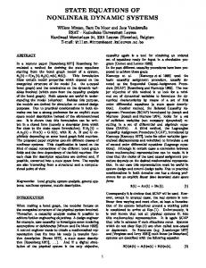
The score generated by an excerpt of music created using the Lorenz equations can be found in Figure 8. As one can see, there are general patterns which are almost repeated in the melody – that is, they are similar, but not exact replicas. In addition, even where a pattern is repeated (for instance, in line 10, the pattern d4. e 8 d4. e 8 is repeated twice), the chord changes, providing a different feel to the same notes. The score generated by an excerpt of music created using the Henon equations can be found in Figure 7. As one can see, the Henon map jumps around in different octaves. This is indicative of the erratic behavior of the Henon map in that, if one were to look at the actual data used to recreate the attractor (Figure 3a) as well as to create the music, one would see very erratic movement between positive and negative, high decimals to low decimals, etc. This is very plainly seen and heard in the musical score and the music respectively. The score generated by an excerpt of music created using the Chua circuit can be found in Figure 6. As one can see, the Chua circuit suddenly jumps from one loop to the other as visualized in the attractor (Figure 4) and in the first line of the score. There are many more switches as can be seen by looking for changes or jumps in the octave. This happens many, many times throughout the piece and can easily be heard, which is another testament to the utility of music in interpreting chaotic behavior in a nonlinear dynamic system such as the Chua circuit.
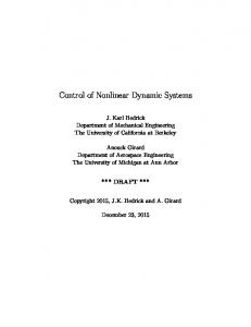
Figure 1: Bifurcation Diagram of the Henon map
5
Discussion
The fact that chaos can be audibly rendered means that one can catch slight differences between two attractors – even if one cannot see the difference. In addition, it is easier to listen 10
Figure 2: Chua’s circuit
(a) Henon map attractor
(b) Logistic map attractor
Figure 3: Attractors
11
Figure 4: Chua’s Attractor
Figure 5: The Chua circuit built at the Naval Sea Systems Command in Philadelphia
12
Chua circuit composition excerpt Last 23 lines
3
� �
� � ����
Chiraag Nataraj
� � � ��� �
3
� � �
� �� �
3
� ����
� �� � � � ��� �
��
� � � � � � � ��� �� ������ ���
� � � � ���� ���� ° ° ���� �
���� �
����� �� �� ���� �� �� � � � � � � � � � � � � � � � � ��� �� �� �� ��� ���� ���� ���� ° ���� �� �� �� � � � �
� � � � � � �
���� �� ������ ��
� � � � � ��� � � �� ° �� �� ���� �� ° � � � � � �� � �� � � � � � � � ���� ���� ���� � �
� � �� � �� � �� � � � �
��
� � � � �� �� ° �� � �� �� �� �� ���� ��� ��� �� � � � � � � � � � �
������ �� ������ �� � � 3 � � � �� �� �� � � �� �� � ��� � ���� �� ��� ��� ���� � ��� � � � � � � � � � �� � �� � � � �� � � � � � �
3 � � � � � � � � � ��� ��� � ° �� ��� ° ���� ° � � ���� ���� � � ° �� � �� � � ����
Figure 6: The score from an excerpt of the music generated by Chua’s circuit
13
Henon map composition excerpt First 20 lines
©
H H � �
H
H
H
Chiraag Nataraj
� H H H �
H
H
H
H
H
�
HH � �� �� HHHH HH � � � � H H H H H � H H � H � H H � H H H � HHHH HHHH HHHH HHHH � ���� � � ���
� � � H H H H H H H H � H � H � H H � H � H H H � � ����
©
� � � ���� �
H
� ���� �
H
H
� H H H
�
� ����
H
� � ����
H
H
H
� H
� ����
�
�
H H H H H
H
H H H H H
����
H � H H
�
H
� H
H
H
� H
H �
�
� H
HH HH
H
HHHH �
H
H HHH � ���� �
H H
�
HHHH ���� � H
H H
HHH �� H �� �
HHHH �
14
H
H H H H
H H
H
H � H H
����
H� H
� H
H
� � H
H
�
�
H
HHHH � � H �
HHHH HHHH
� �H H � H � HHHH �
H� H HHHH � �H
H
H H HHH �
2
H � � � � ���� H � © � � �� ���
H � �� � ���
H
H
H
�
�
H H H H
H
H
� H
H
H
H
� H
H
H
H
H
� H
� H
HHHH HHHH ���� �
� H H
HHHH ���� �
� H
HH � �� HH �� �
H
H
H
H
H
H
H H H
� H
H � �
�
H
� H
�
H H H
� � � H
H
HHHH �
HHHH �
H HHHH �
Figure 7: The score from an excerpt of the music generated by the Henon equations
15
Lorenz equations composition excerpt Last 31 lines
� �� �
Ú
Chiraag Nataraj
=
� � � ���� Ú
�
�
�
� � �� ���
� � �
����
�
�
�
� �� ��
� � � � � ����
� � �
� �
Ú
�
� � � ����
� � � � � �� ���
�
�
� �
=
����
����
� �� �
� �
=
� �� �
=
� � � ���� ���� � �� �
=
�
� � �
� �
�� �� �
���� ���� � �
�
��
��
�
�
16
�
� � �
� ��� �
=
�� �
�
=
� �
�
�
� � � � �
� ���
�� �� �
� � � �
� ���
���� �
�
���� ���� �
� � �
��� �
� � �
�
� � � � � � �
��� �
� � �� � � � � � � � �
�
�
���� ���� ���� �
���� ���� � � ���� �
�
� � �
�
�� �
� � � �
=
=
����
���� �
�� �� �
�� �� �
� � �
2
� � � � � ���� Ú
� � � � ����
Ú
�
� ��� �
�
� � � � �� ��� �
�
Ú
� ���� �
� ����
� � � � �
�
�
�
=
�
� �� � �
� � �
� �
�
� �
� � � �� ��
� � �
� �
� �
�� �
=
� �
��� �
=
� � � � � � ��� � �
�
�
�
�
�
�
�
�
=
�
�
�
� �
�
�
�
�� � ��� � �
=
� �
���� ���� �
�� � � � �
�� � �� �� �� � � � �
=
�
=
�� �
� �
� � �
� �
���� � �
� � ��� �
�
�� �
����
� �� ��
�
� �� �� �� �� � �
� � � �
� �
�
�
����
�
�
�
��� � �
� ����
���� ���� �
� �
����
�
� � � ���� � �
��� � � ��� � � �
���� � ���� �
Figure 8: The score from an excerpt of the music generated by the Lorenz equations
17
for a difference while, say, operating machinery, than it is to look for a change. The current work is very different from the work of the other people who have worked on this in that this work has brought the element of jazz and chord progressions into the music, which no one else has done. It has also brought in the idea of chord progressions, which, until now, had not been done. The few people who have done this sort of work have not done anything to do with jazz, scales, chords, etc. These features bring in a lot more variability and richness into the music; moreover, it brings in added complexity that is absolutely necessary to interpret the complex behavior of nonlinear dynamic systems.
6
Conclusion and Future Plans
In conclusion, this project provides an excellent means of understanding nonlinear dynamic systems through music. After extensive review of previous work in this area, it was found that the nonlinearity of a system was used either to modify existing music, not providing a window into the complex dynamics of the system, or to generate simplistic music, again, not completely representing the dynamics of the system. On the other hand, this project enabled better interpretation of the underlying nonlinear mechanics of the system through the creation of new music that was significantly more sophisticated than the previous work, thus providing more details about the intricate dynamics. Data acquisition from a Chua circuit was implemented using LabView software and the data collected was parsed using Java. The created music also consisted of more advanced concepts such as chord progressions and modes which are representative of the location of points on the strange attractor, a pattern along which the data points in the chaotic system will fall. The chord progression changes help immensely with interpreting chaos, as one can hear the dissonance. Also, the music is created from a musician’s perspective in that the chord progressions are modeled after a jazz concept, where musicians navigate in and out of a scale during the course of a rendition. A couple of questions still remain. • Can one truly represent all of the intricacies of chaos using music? Significant work needs to be done in order to answer this burning question. • Could this also be an effective means of creating sophisticated, beautiful, and versatile music autonomously? This project tried to partially accomplish this by staying within a scale (C Major), but it is not sufficient just to stay within the scale because there can be durational or octaval issues. Notes jumping too quickly jar the nerves, while really slow music can bore the listener. This project also tried to ensure that there were not too many fast or slow notes by keeping the longest duration a quarter dotted note. However, this is still programming in what humans believe sounds good, whereas the question is whether the computer can tell what sounds good and only play or otherwise output only that music. • Is it possible to explore application to Indian classical music which has been a passion for me (both vocal and tabla)? Indian classical music emphasizes melody (raaga) and rhythm as opposed to chords; my suspicion is that this would represent quite a challenge. 18
A possible future goal for this project could be improving the aesthetic quality of the music by adding a rhythm to make it even more musical while also giving the song a much stronger beat. Also, more complex musical elements such as multiple melodies, staccato, legato, tempo, etc could be implemented in order to facilitate interpretation of multiple linked mutually dependent systems. If I were to start this project today, I would spend more time planning the feature set and prioritizing them better.
19
References [1] Eleonora Bilotta, Stefania Gervasi, and Pietro Pantano. Reading Complexity In Chua’s Oscillator Through Music. Part I: A New Way Of Understanding Chaos. International Journal of Bifurcation and Chaos, 15(2):253–382, 2005. [2] Diana S. Dabby. Musical variations from a chaotic mapping. Chaos, 6(2):95–107, 1996. [3] David Little. Composing with chaos; applications of a new science for music. Interface, 22:23–51, 1993.
20