Complexity issues on Newton sums of polynomials ´ Alin Bostan, STIX, Ecole polytechnique 91128 Palaiseau, France
[email protected] Laureano Gonzalez-Vega, Universidad de Cantabria 39005 Santander, Spain
[email protected] Herv´e Perdry, Universidad de Cantabria 39005 Santander, Spain
[email protected] ´ ´ Eric Schost, STIX, Ecole polytechnique 91128 Palaiseau, France
[email protected] Abstract We consider the following problem: given the first d Newton sums of a degree d polynomial P , recover the coefficients of P . We propose fast algorithms to perform this conversion for polynomials over the p-adic ring Zp . As an application, we deduce a new algorithm to compute the composed product of polynomials over the finite field Fp , whose bit-complexity improves the known results by a factor of log d in many cases.
1
Introduction
Univariate polynomials are usually represented by their coefficients in the monomial basis. An useful alternative representation is provided by the power sums (or Newton sums) of their roots. For instance, this representation was used for algorithmic purposes by [9] to speed-up the computation of a special kind of bivariate resultants, the composed products. For us, this is a typical example of an operation on univariate polynomials for which the Newton sums provide the appropriate data structure of the input polynomials. Other applications of Newton sums concern the computation of characteristic or minimal polynomials [19, 28, 31], the manipulations of symmetric functions in the context of algebraic elimination [18, 32, 11, 14, 12, 13, 25, 6], polynomial factorization [33], etc. Let k be a field and let P be a polynomial of degree D in k[X]. The coefficients of P are uniquely determined by the first D power sums of its roots, at least if k has characteristic zero or larger than D. If k has positive characteristic p, the one-to-one correspondence between Newton sums and coefficients is no longer valid. However, under the stronger hypothesis that the multiplicities of all the roots of P are less then p, the first 2D power sums of P suffice to uniquely determine its coefficients. From the computational point of view, one is interested to perform efficiently the conversions between the two representations. Newton formulas, which relate coefficients to power sums of
1
roots, provide a straightforward algorithm to make these conversions, which has quadratic complexity in the degree D. Fortunately, faster conversion methods exist. As far as we know, Sch¨ onhage [27] was the first to propose such a method, in the context of devising numerical root-finders for univariate polynomials. Over fields of characteristic zero, his algorithms extend to an exact setting as well, see [21, Appendix A] and [1, Problem 4.8]. Moreover, Schnhage’s algorithm for translating a polynomial to its Newton representation remains valid over fields of any characteristic, while his algorithm for the converse direction works over fields of characteristic large enough. The question of converting power sums of roots to coefficients for polynomials over fields of small characteristic is more delicate and many efforts have been done to bypass its difficulty. Historically, two kinds of approaches were proposed: on the one hand, the techniques of recursive triangulation originated by [16], on the other hand, those using fundamental sets of power sums of [28, 1, 22, 24]. The best currently known solution is that of [24]. In this paper, we restrict to a class of fields of positive characteristic, including the finite field Fp . We consider the following kind of situation: one is given some polynomials in Fp [X] and wants to perform an operation on them whose result also lies in Fp [X]. We suppose moreover that for this operation the representation by Newton sums is appropriate, that is, it has a simple interpretation on the coordinates of the input polynomials in the new representation.
2
Notation
Arithmetic complexity. To give complexity estimates over a ring R, we introduce a function M : N → N such that M(d) denotes the complexity of degree d polynomial multiplication in R[X], in terms of number of operations (+, −, ×) in R. We suppose that the multiplication time function M verifies the inequality M(d1 ) + M(d2 ) ≤ M(d1 + d2 ) for all positive integers d1 and d2 ; in particular, the inequality M(d/2) ≤ 1/2 M(d) holds for all d ≥ 1. We also make the hypothesis that M(cd) is in O(M(d)), for all c > 0. The basic examples we have in mind are classical multiplication, for which M(n) ∈ O(n2 ), but also fast multiplication algorithms like Karatsuba’s [17] with M(n) ∈ O(n1.59 ). Better, using Fast Fourier Transform (FFT) algorithms, we have M(n) ∈ O(n log n) if the base ring has enough primitive roots of unity, and M(n) ∈ O(n log n log log n) unconditionally [29, 26, 8]. Our references for matters related to polynomial arithmetic are the books [1, 7, 10]. Bit complexity. Let next Mint : N → N denote the complexity of integer multiplication, such that two numbers of bit-size b can be multiplied in Mint (b) bit operations. Using FFT algorithms, Mint (b) ∈ O(b log b log log b)). The following lemma gives the main properties used in the sequel. Lemma 1. Let M in N and R = Z/M Z. Then: • All operations (+, −, ×) in R can be performed for Mint (log M ) bit operations. • If a, b are in R and b divides a in R, then one can compute c in R such that a = bc in Mint (log M log log M ) bit operations. Proof. See [10, Corollary 11.10]. Others. Let P be the power series Pb i i=a pi X .
P
i≥0 pi X
i.
2
The notation [P ]ba designates the polynomial
3
Basics on Newton sums
We begin by recalling some useful results concerning Newton sums of polynomials. The next lemma gathers together the most basic facts that will be used in the sequel. These results are classical; for instance, the equalities in (ii) are commonly known as Newton’s formulas and those of (iv) as Waring’s formulas [20], see also [4, Ex. 6, §6, Ch. A IV]. Lemma 2. Let let P = X d + A1 X d−1 + · · · + Ad be a monic polynomial in F [X] P F be a field, and let Si = P (x)=0 xi be its Newton sums, for i ≥ 1. Let P ∗ be the reciprocal polynomial of P . Then: P (i) the power series expansion of (P ∗ )0 /P ∗ in F [[X]] equals − i≥0 Si+1 X i . (ii) for any 1 ≤ i ≤ d, the equality iAi + S1 Ai−1 + · · · + Si = 0 holds. (iii) for any 1 ≤ i ≤ d, the Newton sums of the polynomial X i +A1 X i−1 +· · ·+Ai are S1 , . . . , Si respectively. (iv) for all i ≥ 1, the following formula holds Si = i
X
(−1)µ1 +···+µr
µ1 θ1 + · · · + µr θr = i µ1 > 0, . . . , µr > 0 θr > · · · > θ1 > 0
(µ1 + · · · + µr − 1)! µ1 Aθ1 · · · Aµθrr . µ1 ! · · · µr !
Q Proof. (i) Let x1 , . . . , xd be the roots of P in an algebraic closure of F . Then P ∗ = di=1 (1 − P P xi xi X), so its logarithmic derivative equals di=1 − 1−x = − di=1 (xi + x2i X + x3i X 2 + . . . ). The iX P latter sum is equals − i≥0 Si+1 X i , and this proves the first assertion. i−1 on both hands of the equality (P ∗ )0 = (ii) simply P follows byi equating the coefficients of X ∗ P × (− i≥0 Si+1 X ) in F [[X]].
(iii) is a direct consequence of (ii). (iv) We will show that the generating series of the sequences on both sides of the formula are equal. by formally integrating the equality at point (i), we deduce that thePgenerating seP First, Si i ries i≥1 i X equals −ln(P ∗ ). On the other hand, using the Taylor expansion i≥1 (−1)i X i /i of −ln(1 + X), we see that −ln(P ∗ ) =
X (−1)µ (A1 X + · · · + Ad X d )µ µ
µ
.
Now, the multinomial formula shows that the monomials of degree i that appear in the right-hand of the previous sum are µ ¶ µ1 d µd µ1 +···+µd µ1 + · · · + µd (A1 X) · · · (Ad X ) (−1) µ1 + · · · + µd µ1 , . . . , µd for all d-tuples (µ1 , . . . , µd ) of non-negative integers such that i = µ1 + 2µ2 + · · · + dµd . Up to a convenient renumbering of the indices, this finishes the proof of the last assertion.
3
4
The fundamental inequality
Let p be a prime and Zp the ring of p-adic integers and Qp the field of p-adic numbers, the p-adic valuation being denoted by v( · ). Note that v(xy) = v(x) + v(y) for all x, y ∈ Qp and also that v is non-archimedian, that is, v(x + y) ≥ min{v(x), v(y)}, for all x, y ∈ Qp . Let us also define w : N>0 → N by w(i) = blogp (i)c; in other words, w(i) is characterized by the inequalities pw(i) ≤ i < pw(i)+1 . Note that for i ≥ 1 we have that v(i) ≤ w(i); note also that w is increasing and verifies the inequality w(x) + w(y) ≤ w(xy), for all x, y ≥ 1. We state now the crucial inequality on which are based all the results of this paper. Intuitively, it asserts, in its simpler form (see Corollary 1 below), that two polynomials over Zp whose Newton sums are close with respect to the p-adic topology, also have their coefficients almost as close. In the sequel, we will actually need the stronger version that we state now. Theorem 1. Let P and Q in Qp [X] be two monic polynomials of degree d, with P = X d + A1 X d−1 + · · · + Ad ,
Q = X d + B1 X d−1 + · · · + Bd .
Let (Si )i≥1 and (Ti )i≥1 be the Newton sums of P and Q: X X xi . xi , Ti = Si = Q(x)=0
P (x)=0
Let 1 ≤ i ≤ d and α ∈ N be such that • v(Si − Ti ) ≥ α; • for all 1 ≤ j < i, Aj and Bj are in Zp and v(Aj − Bj ) ≥ α − w(j). Then the inequality v(Ai − Bi ) ≥ α − w(i) holds. Proof. We start by a lemma; by convention, the empty product equals 1. Lemma 3. Let r ≥ 0, let X1 , . . . , Xr and Y1 , . . . , Yr be indeterminates over P Z. For any r-uple µ1 µr µ1 µr r (µ1 , . . . , µr ) in N , the polynomial X1 · · · Xr − Y1 · · · Yr can be written ri=1 ∆i (Xi − Yi ), with ∆i ∈ Z[X1 , . . . , Xr , Y1 , . . . , Yr ] for i = 1, . . . , r. Proof. We proceed by induction on r, the case r = 0 being obvious. Suppose now that the result holds for some r ≥ 0; we prove it for r + 1. Let us then consider a product of the form µr+1 µr+1 X1µ1 · · · Xr+1 − Y1µ1 · · · Yr+1 . We rewrite it as µ
µ
µ
r+1 r+1 r+1 X1µ1 · · · Xrµr (Xr+1 − Yr+1 ) + Yr+1 (X1µ1 · · · Xrµr − Y1µ1 · · · Yrµr ).
µ
µ
r+1 r+1 To deal with the first term, we rewrite (Xr+1 −Yr+1 ) as (Xr+1 −Yr+1 ) The second term is dealt with using the induction hypothesis.
Pµr+1 −1 i=0
µ
i Y r+1 Xr+1 r+1
−i−1
.
Applying the last part of Lemma 2 for both polynomials P and Q, we obtain by subtraction Si − Ti = i
X µ1 θ1 + · · · + µr θr = i µ1 > 0, . . . , µr > 0 θr > · · · > θ1 > 0
(−1)µ1 +···+µr
(µ1 + · · · + µr − 1)! µ1 (Aθ1 · · · Aµθrr − Bθµ11 · · · Bθµrr ). µ1 ! · · · µr !
4
In this sum, the term corresponding to r = 1, θr = i, µr = 1 equals −(Ai − Bi ). Rewriting the formula to isolate this term shows that Ai − Bi is given by Ti − Si + i
X
(−1)µ1 +···+µr
µ1 θ1 + · · · + µr θr = i µ1 > 0, . . . , µr > 0 i > θr > · · · > θ1 > 0
(µ1 + · · · + µr − 1)! µ1 (Aθ1 · · · Aµθrr − Bθµ11 · · · Bθµrr ). (1) µ1 ! · · · µr !
Now, using Lemma 3, and the fact that the coefficients A1 , . . . , Ai−1 and B1 , . . . , Bi−1 are in Zp , we remark that any term of the form Aµθ11 · · · Aµθrr −Bθµ11 · · · Bθµrr belongs to Zp [Aθ1 −Bθ1 , . . . , Aθr − Bθr ]. Thus, the sum in Formula (1) can be written X ¢ (µ1 + · · · + µr − 1)! ¡ (θ,A,B) (−1)µ1 +···+µr c1 (Aθ1 − Bθ1 ) + · · · + c(θ,A,B) (Aθr − Bθr ) , r µ1 ! · · · µr !
(2)
θ,µ
(θ,A,B)
for some coefficients ci ∈ Zp , and where θ = (θ1 , . . . , θr ) and µ = (µ1 , . . . , µr ) satisfy the same conditions as in Formula (1). Regrouping terms, we deduce an equality of the form Ai − Bi =
X Ti − Si + γj (Aj − Bj ), i
(3)
1≤j 0 for 1 ≤ k ≤ r and µ1 θ1 + · · · + µr θr = i, be such that θk = j for some 1 ≤ k ≤ r. The corresponding coefficient µk then satisfies the inequality jµk = θk µk ≤ i. The inequality w(x) + w(y) ≤ w(xy), valid for all x, y ≥ 1, shows that w(j) + w(µk ) ≤ w(jµk ). Since w is increasing, we deduce that w(µk ) is bounded from above by w(i) − w(j), which implies that v(µk ) admits the same upper bound. Now, the corresponding term in Formula (2) is (up to sign) (µ1 + · · · + µr − 1)! (θ,A,B) ck (Aj − Bj ), µ1 ! · · · µr ! which we rewrite as µ
¶ µ1 + · · · + µr − 1 (θ,A,B) Aj − Bj (µ,θ,A,B) Aj − Bj = δk , ck µ1 , . . . , µk − 1, . . . , µd µk µk
(µ,θ,A,B)
where δk belongs to Zp . Due to our previous upper bound on v(µk ), the valuation of the above term admits the lower bound v(Aj −Bj )−w(i)+w(j); by our assumptions, this is bounded from below by α − w(i). Summing all such contributions, and using that v is non-archimedian, we deduce that the valuation of γj (Aj − Bj ) admits the same lower bound. i Next, recall that by assumption, v( Ti −S i ) = v(Ti − Si ) − v(i) ≥ α − v(i); since v(i) ≤ w(i), Ti −Si we obtain the inequality v( i ) ≥ α − w(i). Finally, we can deduce from Equation (3) and the above discussion the inequality v(Ai − Bi ) ≥ α − w(i). This concludes the proof. A straightforward consequence of Theorem 1 is the following corollary which will not be used in the sequel, but which merits however to be stated. Intuitively, it asserts that two polynomials over Zp whose Newton sums are close with respect to the p-adic topology, also have their coefficients almost as close. 5
Corollary 1. Let P and Q in Zp [X] two monic polynomials of degree d, with P = X d + A1 X d−1 + · · · + Ad ,
Q = X d + B1 X d−1 + · · · + Bd .
Let (Si )i≥1 and (Ti )1≤i≤d be the Newton sums of P and Q and let α ∈ N be such that v(Si − Ti ) ≥ α,
for all 1 ≤ i ≤ d.
Then the inequality v(Ai − Bi ) ≥ α − w(i) holds for all i ≥ 1.
5
Algorithms
Let P be in Zp [X], with P = X d + A1 X d−1 + · · · + Ad , let (Si )i≥1 be its Newton sums. The aim of this section is to propose efficient algorithms which, given the Newton sums of P truncated at a certain precision α > 0, recover the coefficients of P at some smaller, but still positive precision. An immediate algorithm allows to do this via Newton’s formulas, provided that we work at initial precision α = O(d). Indeed, the ith Newton formula (see Lemma 2, ii ) involves a division by i, so that after using it to compute Ai , a precision v(i) is potentially lost. Since Pd i=1 v(i) = v(d!) ≈ d/(p − 1), it may thus appear that an initial precision of computations linear in d is needed to ensure that, at the end, all the Ai ’s are recovered at some positive precision. In terms of computational amount of work, this algorithm would require O(d2 ) operations (+, −, ×, ÷) in Z/pα Z, where α = O(d/p), hence a bit-complexity at least of order O(d2 Mint ( dp log p)) after Lemma 1. In this section we propose two faster algorithms. Our first contribution is to show that the algorithm sketched above (and based on Newton’s relations) already works if we compute only at precision O(logp (d)). This is a non-trivial and quite surprising result, based on Theorem 1. As a direct consequence, the resulting algorithm has a smaller bit-complexity, that is, within O(d2 Mint (log d)) bit operations. Our second algorithm relies on the use of a formal Newton operator with quadratic convergence and is designed to be employed in conjunction with the fast multiplication routines. This algorithm also requires to work only in precision O(logp (d)). Its bit-complexity is in O(M(d) Mint (log d)). Thus, if the FFT-based polynomial multiplication is used, it is faster than the first algorithm by an order of magnitude. In what follows we use the following limpid notations: we let α ≥ w(d) be the precision of computations and let R = Zp /pα Zp be the ring of p-adic integers truncated at precision α. Since it is isomorphic to Z/pα Z, we will make no distinction between these two rings. For i ≥ 1, we define si and ai in R by si = Si mod pα and ai = Ai mod pα .
5.1
The quadratic algorithm
The first result proves that the loss of precision during the successive divisions by 1, 2, . . . , d in the algorithm based on Newton formulas does not exceed w(d). This is quite surprising, since it replaces the a priori pessimistic bound v(d!), which is linear in d/p, by a bound which is linear in logp (d). From the computational view-point, this enables to save precision and thus to improve the bit-complexity of the algorithm based on Newton formulas. Theorem 2. Let 1 ≤ k < d and let a1 , . . . , ak be in R such that the equality iai + s1 ai−1 + · · · + si = 0 holds for i = 1, . . . , k. Then: (i) There exists ak+1 in R such that (k + 1)ak+1 + s1 ak + · · · + sk+1 = 0. (ii) Any such ak+1 satisfies the equality ak+1 = ak+1 mod pα−w(k+1) . 6
Proof. Let A1 , . . . , Ak be arbitrary lifts of a1 , . . . , ak in Zp , and let Ak+1 ∈ Qp be defined by the relation (k + 1)Ak+1 + S1 Ak + · · · + Sk+1 = 0. To prove point (i), we show that Ak+1 is in Zp ; this will be done by proving the stronger assertion that Ak+1 satisfies the inequality v(Ak+1 − Ak+1 ) ≥ α − w(k + 1). To this effect, we introduce two polynomials Pk and Q, and consider their Newton sums: • Let first Pk be the polynomial X k+1 + A1 X k + · · · + Ak+1 ; by Lemma 2, the first k + 1 Newton sums of Pk are S1 , . . . , Sk+1 . • Let next Q ∈ Qp [X] be the polynomial X k+1 + A1 X k + · · · + Ak+1 and let T1 , . . . , Tk+1 be its first k + 1 Newton sums. Then, for i = 1, . . . , k + 1 we have simultaneously v(iAi + S1 Ai−1 + · · · + Si ) ≥ α
and iAi + T1 Ai−1 + · · · + Ti = 0.
Since Ai is in Zp for i = 1, . . . , k, we deduce by successive subtractions that v(Si − Ti ) ≥ α for i = 1, . . . , k + 1. Applying inductively Theorem 1 to Pk and Q for all indices i = 1, . . . , k + 1, we obtain the inequalities v(Ai − Ai ) ≥ α − w(i). In particular, since α ≥ w(k + 1), we deduce that Ak+1 is in Zp . Let then ak+1 = Ak+1 mod pα : we see that (k + 1)ak+1 + s1 ak + · · · + sk+1 = 0, proving point (i), and that furthermore ak+1 = ak+1 mod pα−w(k+1) . We now prove point (ii). Let then ak+1 be any element of R such that (k + 1)ak+1 + s1 ak + · · · + sk+1 = 0. By subtraction, we deduce that (k + 1)(ak+1 − ak+1 ) = 0. This implies that pv(k+1) (ak+1 − ak+1 ) = 0; since v(k + 1) ≤ w(k + 1), we deduce that pw(k+1) (ak+1 − ak+1 ) = 0. In other words, ak+1 = ak+1 mod pα−w(k+1) ; since we also have ak+1 = ak+1 mod pα−w(k+1) , we obtain ak+1 = ak+1 mod pα−w(k+1) , concluding the proof. Corollary 2. Let f ∈ Zp [X] be a monic polynomial of degree d. Knowing the first d Newton sums of f at precision α = blogp (d)c + 1, its coefficients can be computed at precision 1 using ¡ ¢ O d2 Mint (log d) bit operations. Proof. By Theorem 2, the algorithm described in Figure 1 is correct and requires O(d2 ) operations (+, −, ×) in Z/pα Z and d exact divisions. Lemma 1 finishes the proof.
5.2
The fast algorithm
We present now a fast algorithm to perform the conversion between Newton sums and coefficients. It is based on the classical fact that this conversion mainly amounts to exponentiate the primitive of the generating series of the Newton sums (as can be seen from point (ii) of Lemma 2). Now, nearly optimal algorithms to compute exponentials of power series have been given by [5] (and already used in [27] for this purpose). They use a formal version of Newton’s operator, whose quadratic convergence ensures the good complexity behaviour. Thus, in principle, a fast version of our algorithm is possible, the only problem concerns the divisions occurring during the algorithm. More specifically, each iteration of Newton’s operator involves a primitive computation. Thus, in order to control the loss of precision, we must deal with these divisions. The following theorem shows that, as in the case of the quadratic algorithm, a precision of at most w(d), that is, logarithmic in d, is lost during the Newton’s iterations. This result allows to obtain a faster (in terms of bit-operations) algorithm than the algorithm described in Section 5.1. 7
Recovering a monic polynomial from its Newton series Input: the Newton sums s1 , . . . , sd of f in R = Zp /pα Zp Output: the coefficients of f in Fp = Zp /pZp . a1 ← −s1 for k from 1 to d¡ − 1 do ¢ 1 ak+1 ← − k+1 s1 ak + · · · + sk a1 + sk+1 P return the image of F = X d + di=1 ai X d−i in Fp [X]
Figure 1: Recovering a monic polynomial from its Newton sums in small characteristic using Newton’s formulas Theorem 3. Let k ≥ 1 and let a1 , . . . , ak be in R such that ai = ai mod pα−w(i) for 1 ≤ i ≤ k. Let K = min(2k + 1, d) and let g and δ in R[X] be the polynomials k
g = 1 + a1 X + · · · + ak X ,
δ=−
K−1 X i=k
· 0 ¸K−1 g si+1 X − . g k i
Then: (i) There exists h ∈ R[X] such that h0 = δ. (ii) Let h be such that h0 = δ and h(0) = 0, and let f = g(1 + h) mod X K+1 in R[X]. Then f has the form 1 + a1 X + · · · + aK X K , and ai satisfies the equality ai = ai mod pα−w(i) for 1 ≤ i ≤ K. Proof. First, we prove the existence of h in R[X] which simultaneously satisfies the conditions of points (i) and (ii). To this effect, let G be a lift of g in Zp [X] of the form 1 + A1 X + · · · + Ak X k , and let · 0 ¸K−1 K−1 X G i ∆=− Si+1 X − ∈ Zp [X]; G k i=k
note that δ = ∆ mod pα . Let now H ∈ Qp [X] be such that H 0 = ∆ and H(0) = 0; let also F = G(1 + H) mod X K+1 ∈ Qp [X], and note that F has the form 1 + A1 X + · · · + AK X K . To establish our claim, it suffices to prove that: • H and F are in Zp [X]; • v(Ai − Ai ) ≥ α − w(i) for i = 1, . . . , K. Indeed, the polynomials h = H mod pα and f = F mod pα are then seen to satisfy the conditions of point (ii). Let us consider the logarithmic derivative of F in Qp [[X]]: first, the definition F = G(1 + H) mod X K+1 yields the equality F0 G0 H0 = + F G 1+H 8
mod X K .
Since H 0 = ∆ and H has valuation at least k + 1, this implies G0 F0 = + ∆ mod X K ; F G in particular, considering the coefficients of degrees k, . . . , K − 1 shows that · 0 ¸K−1 K−1 X F =− Si+1 X i . F k
(4)
i=k
We now define two polynomials F ∗ and Pk , and study their Newton sums: • Let first PK be the polynomial X K +A1 X K−1 +· · ·+AK ; by Lemma 2, the first K Newton sums of PK are S1 , . . . , SK . • Let next F ∗ = X K + A1 X K−1 + · · · + AK be the reciprocal polynomial of F and let T1 , . . . , TK be its first K Newton sums. In view of Equation (4), we deduce from Lemma 2 that Ti = Si for i = k + 1, . . . , K. Thus, the Newton sums of PK of indices k + 1, . . . , K coincide with those of F ∗ . On the other hand, our assumption on a1 , . . . , ak shows that v(Ai − Ai ) ≥ α − w(i) for i = 1, . . . , k. We then apply inductively Theorem 1 to F ∗ and PK , for i = k + 1, . . . , K: for any such i, this yields the inequality v(Ai − Ai ) ≥ α − w(i), and thus that Ai is in Zp , since α ≥ w(i). Thus, F is in Zp [X]. Since G is invertible in Zp [[X]], we deduce that H is in Zp [X] as well. Letting h = H mod pα , we see that h satisfies the conditions of points (i) and (ii). Let us now complete the proof, by establishing point (ii). Let thus h be any polynomial in 0 R[X] such that h(0) = 0 and h = δ, and let f = g(1 + h) mod X K+1 , so that the difference f − f equals g(h − h) mod X K+1 . P i The polynomial λ = h − h satisfies λ0 = 0 in R[X]; writing λ = K i=k+1 λi X , this means w(i) λ = 0 as well since v(i) ≤ w(i). that λi satisfies pv(i) λP i = 0 for i = k + 1, . . . , K, and thus p i K i Let us write f − f = i=k+1 Λi X ; since f − f = g(h − h) mod X K+1 and w is increasing, we see by expanding the product that pw(i) Λi = 0 for i = k + 1, . . . , K. This finishes the proof of the theorem. Corollary 3. Let f ∈ Zp [X] be a monic polynomial of degree d. Knowing the first d Newton sums of f at precision α = blogp (d)c + 1, its coefficients can be computed at precision 1 using ¡ ¢ O M(d) Mint (log d) bit operations. Proof. Theorem 3 shows that the algorithm described in Figure 2 is correct and that it requires Plog2 (d) O(M(2i )) = O(M(d)) operations (+, −, ×) and O(d) exact divisions in Z/pα Z. The i=1 result follows from Lemma 1. Remark. Without using Theorem 3, we are able to prove only a weaker version of Corollary 3. That version is not sufficient to our purposes, since it would require as input the first d Newton 2 0 sums of f at precision of α = O(log d) and would have a bit-complexity ¡ α = O(log 2d) instead ¢ upper bounded by O M(d) Mint (log d) . Indeed, an immediate count of the divisions performed by the fast algorithm in Figure 2 shows that at the ith iteration, only divisions by 1, 2, . . . , 2i occur, so a precisionPof at most w(2i ) could be lost. ¡ 2Thus, an a ¢priori bound of the total needed i precision would be i≤log d w(2 ), which is in O log d/ logp (d) . As in the case of the quadratic algorithm, these bounds are pessimistic compared to those provided by the more refined results in Corollary 3. 9
Recovering a monic polynomial from its Newton series Input: the Newton sums s1 , . . . , sd of f in R = Zp /pα Zp Output: the coefficients of f in Fp = Zp /pZp S ← s1 + s2 T + · · · + sd T d−1 g←1 prec ← 1 while prec ≤ d − 1 do h 0 iMin(prec,d−1) δ ← − gg + S prec/2 P i h ← i≥1 Coeff(δ, i − 1) Ti g ← dg(1 + h)e2×prec prec ← 2 × prec f ← rev(g) return the image of F in Fp [X]
Figure 2: Recovering a monic polynomial from its Newton sums in small characteristic using Newton’s iteration
5.3
Previous work
Let us compare the complexity of our second algorithm to the other results existing in the literature. The previous fastest known algorithm for recovering a polynomial from its Newton sums in small characteristic is due to Sch¨ onhage and Pan [28, 22, 23, 24]. As input, this algorithm requires the first 2d Newton sums of f ; it works under the assumption that all roots of f have multiplicities less than p. This algorithm decomposes in two steps: the first one is quite similar to the fast exponentiation algorithm of [5, 27], which is also the base of our algorithm; the second step consists in p − 1 Pad´e approximant computations in degrees (d/p, d/p). Thus, its arithmetic complexity is O(M(d) + p M(d/p) log(d/p)) operations in Fp , and its bit-complexity is within ³ ¡ ¢´ O M(d) + p M(d/p) log(d/p) Mint (log p). To simplify the comparison, let us suppose that the FFT is used and that M(d) = O(d log d). Thus, the cost of our algorithm is within O(d log2 d log log d) bit operations, while that of Sch¨onhage-Pan’s algorithm is of O(d log2 (d/p) log p log log p) bit-operations. Let p = dβ , with 0 < β < 1. Then the ratio between the two costs equals d(1 − β)2 log2 (d)β log d log(β log d) ≈ β(1 − β)2 log d. d log2 d log log d This estimate shows that is β varies in a fixed range 0 < β0 ≤ β ≤ β1 < 1, our algorithm is faster roughly by a factor of log d. On the other hand, for β ' 0, that is, for constant p, the bit complexity of Sch¨onhage-Pan’s algorithm is within O(M(d) log d), which is better than ours by a log log d factor. Similarly, for β ' 1, that is, when the ratio d/p is constant, the bit 10
complexity of Sch¨onhage-Pan’s algorithm is within O(M(d)Mint (log d)), which is in the same complexity class as our estimates. One should keep in mind that the input of the two algorithms differ. The next section will compare the behavious of the two algorithms for a classical application, composed products.
6
Application: composed products
Let k be a field and let f and g be monic polynomials in k[T ], of degrees m and n respectively. We are interested in computing efficiently their composed product f ⊗ g. This is the polynomial of degree D = mn defined by Y f ⊗g = (T − αβ), α,β
the product running over all the roots α of f and β of g, counted with multiplicities, in an algebraic closure k of k. The algorithm of Figure 3 was initially proposed by Dvornicich and Traverso in characteristic zero; its arithmetic complexity is O(M(D)) operations in k. Composed product Input: f and g in k[T ] Output: f ⊗ g D ← deg(f ) deg(g) S ← [Newtoni (f ) : i ≤ D] T ← [Newtoni (g) : i ≤ D] U ← [Si Ti : i ≤ D] Recover f ⊗ g from its first D Newton sums U Figure 3: Computing a composed product If k has positive characteristic, then the first D Newton sums of f ⊗ g are not enough to recover it. In [2], it is proposed to use Sch¨ onhage-Pan’s algorithm, which requires to compute the first 2D Newton sums of f ⊗ g, and the assumption that the multiplicities of the roots of f ⊗ g are less than the characteristic of k. The arithmetic complexity of this algorithm is dominated by this last part, that is,within O(M(D) + pM(D/p) log(D/p)) operations in k. If ¡ ¢ k = Fp , then the bit complexity is in O(M(D) + p M(D/p) log(D/p) Mint (log p). Now, our algorithm can be used as well in the case k = Fp . The algorithm is a straightforward consequence of the previous considerations; an important difference is that we now have to compute the Newton sums of (arbitrary lifts of) f and g in Z/pα Z[T ] instead of Fp [T ]. As for the Sch¨ onhage-Pan’s approach, the predominant part ¡in the complexity estimate is the last ¢ step; thus, the whole bit-complexity of this approach is O(M(D)Mint (log D) bit operations. In particular, the expected ratio of O(log D) = O(log d) obtained in the previous section when p = dβ and β varies in [β0 , β1 ] carries over to this situation. Experimental results We have implemented our fast algorithm for conversion between Newton sums and coefficients and applied it to the computation of the composed product of polynomials and compared it to the strategy using Sch¨ onhage-Pan’s algorithm.
11
Composed product Input: f and g in Fp [T ] = Z/pZ[T ] Output: f ⊗ g in Fp [T ] = Z/pZ[T ] α ← blogp (d)c + 1 R ← Zp /pα Zp = Z/pα Z Lift f and g to R[T ] D ← deg(f ) deg(g) S ← [Newtoni (f ) : i ≤ D] T ← [Newtoni (g) : i ≤ D] U ← [Si Ti : i ≤ D] Recover f ⊗ g from its first D Newton sums U using Algorithm of Figure 2, and reduce it mod p. Figure 4: Computing a composed product in small characteristic We used the NTL C++ package [30]. The computations are done over base rings of type Z/mZ, where m is a prime power; over such rings, NTL implements polynomial arithmetic using classical, Karatsuba and FFT multiplications. Both algorithms share (up to minor modifications) a common exponentiation step based on a Newton iteration; this step uses the middle product techniques introduced in [15], for which we relied on the implementation presented in [3]. Sch¨ onhage-Pan’s algorithm also requires Pad´e approximant computations; we used NTL’s built-in fast extended GCD routines for this purposes. For the tests presented in Figure 5, the input is formed by two polynomials of equal degree d, whose coefficients are randomly picked in Fp , where p is chosen to be the smaller prime greater than d. Note that the output f ⊗ g has degree D = d2 . We let d vary from 10 to 200, so that D varies from 100 to 40000. All tests were performed on a 500 MB, 2GHz 32 bit Intel processor.
References [1] D. Bini and V. Y. Pan. Polynomial and matrix computations. Vol. 1. Birkh¨auser Boston Inc., Boston, MA, 1994. ´ Schost. Fast computation with two algebraic [2] A. Bostan, Ph. Flajolet, B. Salvy, and E. numbers. Research Report 4579, Institut National de Recherche en Informatique et en Automatique, October 2002. 20 pages. ´ Schost. Tellegen’s principle into practice. In ISSAC’03, pages [3] A. Bostan, G. Lecerf, and E. 37–44. ACM Press, 2003. ´ ements de math´ematique. Masson, Paris, 1981. Alg`ebre. Chapitres 4 `a 7. [4] N. Bourbaki. El´ [5] R. P. Brent. Multiple-precision zero-finding methods and the complexity of elementary function evaluation. In Analytic computational complexity (Proc. Sympos., Carnegie-Mellon Univ., Pittsburgh, Pa., 1975), pages 151–176. Academic Press, New York, 1976. [6] E. Briand and L. Gonz´alez-Vega. Multivariate Newton sums: identities and generating functions. Communications in Algebra, 30(9):4527–4547, 2002. 12
14 Schoenhage-Pan Bostan et al.
12 10 8 6 4 2 0 0
20
40
60
80
100 120 140 160 180 200
Figure 5: Composed product of polynomials over fields of small characteristic. (Input degree on the horizontal axis and time in seconds on the vertical axis.) [7] P. B¨ urgisser, M. Clausen, and M. A. Shokrollahi. Algebraic complexity theory, volume 315 of Grundlehren Math. Wiss. Springer–Verlag, 1997. [8] D. G. Cantor and E. Kaltofen. On fast multiplication of polynomials over arbitrary algebras. Acta Inform., 28(7):693–701, 1991. [9] R. Dvornicich and C. Traverso. Newton symmetric functions and the arithmetic of algebraically closed fields. In AAECC-5 (Menorca, 1987), volume 356 of LNCS, pages 216–224. Springer, Berlin, 1989. [10] J. von zur Gathen and J. Gerhard. Modern computer algebra. Cambridge University Press, 1999. [11] M. Giusti, D. Lazard, and A. Valibouze. Algebraic transformations of polynomial equations, symmetric polynomials and elimination. In P. Gianni, editor, Proceedings of ISSAC’88, volume 358 of LNCS, pages 309–314. Springer Verlag, 1989. [12] M.-J. Gonz´alez-L´opez and L. Gonz´alez-Vega. Newton identities in the multivariate case: Pham systems. In Gr¨ obner bases and applications (Linz, 1998), volume 251 of London Math. Soc. Lecture Note Ser., pages 351–366. Cambridge Univ. Press, Cambridge, 1998. [13] L. Gonz´alez-Vega and G. Trujillo. Implicitization of parametric curves and surfaces by using symmetric functions. In Proceedings of ISSAC’95, pages 180–186. ACM Press, 1995. [14] L. Gonz´alez-Vega and G. Trujillo. Using symmetric functions to describe the solution set of a zero-dimensional ideal. In AAECC-11 (Paris, 1995), volume 948 of LNCS, pages 232–247. Springer, Berlin, 1995. [15] G. Hanrot, M. Quercia, and P. Zimmermann. The Middle Product Algorithm, I. Appl. Algebra Engrg. Comm. Comput., 14(6):415–438, 2004.
13
[16] E. Kaltofen and V. Y. Pan. Parallel solution of Toeplitz and Toeplitz-like linear systems over fields of small positive characteristic. In First International Symposium on Parallel Symbolic Computation—PASCO ’94 (Hagenberg/Linz, 1994), volume 5 of Lecture Notes Ser. Comput., pages 225–233. World Sci. Publishing, River Edge, NJ, 1994. [17] A. Karatsuba and Y. Ofman. Multiplication of multidigit numbers on automata. Soviet Math. Dokl., 7:595–596, 1963. [18] A. Lascoux. La r´esultante de deux polynˆomes. In S´eminaire d’alg`ebre Paul Dubreil et Marie-Paule Malliavin, 37`eme ann´ee (Paris, 1985), volume 1220 of Lecture Notes in Math., pages 56–72. Springer, Berlin, 1986. [19] U. J. J. Le Verrier. Sur les variations s´eculaires des ´el´ements elliptiques des sept plan`etes principales : Mercure, Venus, La Terre, Mars, Jupiter, Saturne et Uranus. J. Math. Pures Appli., 4:220–254, 1840. [20] M. P. Macmahon. Combinatory analysis. Reprinted by Chelsea Publ. Company, 1960. [21] V. Y. Pan. Parallel least-squares solution of general and Toeplitz-like linear systems. In Proc. 2nd Ann. ACM Symp. on Parallel Algorithms and Architecture, pages 244–253. ACM Press, 1990. [22] V. Y. Pan. Parallel computation of polynomial GCD and some related parallel computations over abstract fields. Theoretical Computer Science, 162(2):173–223, 1996. [23] V. Y. Pan. Faster solution of the key equation for decoding BCH error-corecting codes. In Proceedings STOC’97, pages 168–175. ACM Press, 1997. [24] V. Y. Pan. New techniques for the computation of linear recurrence coefficients. Finite Fields and their Applications, 6(1):93–118, 2000. [25] F. Rouillier. Solving zero-dimensional systems through the Rational Univariate Representation. Applicable Algebra in Engineering, Communication and Computing, 9(5):433–461, 1999. [26] A. Sch¨onhage. Schnelle Multiplikation von Polynomen u ¨ber K¨orpern der Charakteristik 2. Acta Inform., 7:395–398, 1977. [27] A. Sch¨onhage. The fundamental theorem of algebra in terms of computational complexity. Technical report, Univ. T¨ ubingen, 1982. 73 pages. [28] A. Sch¨ onhage. Fast parallel computation of characteristic polynomials by Leverrier’s power sum method adapted to fields of finite characteristic. In Automata, languages and programming (Lund, 1993), volume 700 of LNCS, pages 410–417. Springer, Berlin, 1993. [29] A. Sch¨onhage and V. Strassen. Schnelle Multiplikation großer Zahlen. Computing, 7:281– 292, 1971. [30] V. Shoup. NTL: A library for doing number theory. http://www.shoup.net, 1996–2003. [31] J.-A. Thiong Ly. Note for computing the minimum polynomial of elements in large finite fields. In Coding theory and applications (Toulon, 1988), volume 388 of LNCS, pages 185–192. Springer, New York, 1989.
14
[32] A. Valibouze. Fonctions sym´etriques et changements de bases. In Proc. EUROCAL–87, volume 378 of LNCS, pages 323–332, 1989. [33] M. van Hoeij. Factoring polynomials and the knapsack problem. Journal of Number Theory, 95(2):167–189, 2002.
15