1
Complexity of Frictional Interfaces: A Complex Network Perspective
2
H. O. Ghaffari1
3
Department of Civil Engineering and Lassonde Institute, University of Toronto, Canada
4
M. Sharifzadeh
5
Faculty of Engineering, Kyushu University, Hakozaki, Japan
6
E. Evgin
7
Department of Civil Engineering, University of Ottawa, Ontario, Canada
8
Abstract: The shear strength and stick-slip behavior of a rough rock joint are analyzed using the
9
complex network approach. We develop a network approach on correlation patterns of void
10
spaces of an evolvable rough fracture (crack type II). Correlation among networks properties
11
with the hydro -mechanical attributes (obtained from experimental tests) of fracture before and
12
after slip is the direct result of the revealed non-contacts networks. Joint distribution of locally
13
and globally filtered correlation gives a close relation to the contact zones attachment-
14
detachment sequences through the evolution of shear strength of the rock joint. Especially spread
15
of node’s degree rate to spread of clustering coefficient rate yielded possible stick and slip
16
sequences during the displacements. Our method can be developed to investigate the complexity
1
[email protected];
[email protected] Dept. Civil Engineering, U of T, MB108‐170 College Street‐Toronto‐ON‐Canada
1
17
of stick-slip behavior of faults as well as energy /stress localization on crumpled shells/sheets in
18
which ridge networks are controlling the energy distribution.
19
Key words: Frictional interface; Rock joint, Shear strength, Stick-slip, Complex networks,
20
Correlation, Contact areas
21
1. Introduction
22
During the last decade, complex networks have been used increasingly in different fields
23
of science and technology [1-3]. Initial applications of complex networks in geosciences were
24
mostly related to earthquakes [4-6].
25
complexity of such recursive events has been the main objective of the related research [7-13].
26
Understanding of spatio-temporal topological complexity of events based on field
27
measurements can disclose some other facets of these intra/extra woven events.
Characterization of spatial and temporal structural
28
Studies pertaining to the topological complexity and its application in some geoscience
29
fields reveals that acquisition and gathering of direct information (especially in temporal scale) is
30
difficult and in many cases are (were) impossible (at least with current technologies). In addition
31
to complex earthquake networks, recently the analysis of climate networks, volcanic networks,
32
river networks and highway networks, as the large scale measurements, have been taken into
33
account [9-13].
34
geoscience fields such as the gradation of soil particles, fracture networks, aperture of fractures,
35
and granular materials [14-20]. The initial step refers to organizational step which tries to find
36
out possible dominant well-known structures within the system. Next step in the most of the
37
mentioned works is to provide a suitable and simple method to yield a similar structure. Such
38
algorithm may support the evolution of structure in spatial or/and temporal cases [21].
In small scales, topological complexity has been evaluated in relation to
2
39
May be the most important structural complexity in geological fields is related to fracture
40
networks. Fracture networks with dilatancy [22], joint networks in excavation damaged zones,
41
cracking in pavements (or other natural/man-made structures) and fault networks in large scale
42
have been recognized [23-25]. In the analysis of these networks, the characterization of fractures
43
in a proper space such as friction-displacement space is an essential step. Furthermore, with
44
taking the direct relationship between void spaces and contact areas in to account, one may
45
interest in considering the induced topological complexity of the opening elements (non-
46
frictional contacts) into the fracture behavior. Using linear elastic fracture mechanics, we know
47
aperture or aspect ratio is generally the index to available energy in growth of rupture. Crack
48
like behavior of rupture in frictional interfaces also support the role of contact areas and
49
equivalently apertures. In addition, the variations of fluid flow features (such as permeability
50
and tortuosity) directly are controlled with aperture spaces. In order to characterize the main
51
attributes of the fractured systems, e.g. mechanical and hydraulic properties, several methods
52
have been suggested in the literature [26-30]. Recently, the authors have proposed the
53
implementation of a complex network analysis for the evolution of micro-scale apertures in a
54
rough rock fracture [18-19]. Based on a Euclidean measure, the results confirmed the
55
dependency of hydro-mechanical properties to the attributes of characterized aperture networks.
56
The present study is also related to the complex aperture networks. However, the current study
57
presents the analysis of frictional forces during shearing based on the correlation of apertures in
58
a rock joint. The analysis is associated with set up a network on an attribute (such as aperture
59
distribution) in an area. The aforementioned method has also been employed in the analysis of
60
the coupled partial differential equations which was related to two-phase flow [31].
3
61
With respect to avalanche-like behavior of collective motion of the ensemble discrete
62
contacts (in the vicinity of a phase transition step), we try to characterize the collective behavior
63
of aperture strings using networks. In this paper we will answer the following three questions: 1)
64
Is there any (hidden) complex structure in the experimentally observed apertures? 2) What is the
65
effect of specific structural complexity of apertures on mechanical response of a fracture? 3)
66
How do apertures regulate with each other to show well-known slip-friction curve? In other
67
words, can we relate the topological complexity of apertures to the evolution path of the
68
fracture?
69
The organization of the paper is as follows: Section 2 includes a brief description of
70
networks and their characterization. In addition, the construction procedure of aperture networks
71
is explained. Section 3 covers a summary of the experimental procedure. The last section
72
presents the evaluation of the pre- and post-peak (stick-slip) behavior of a rock joint which is
73
followed by the analysis of the constructed network.
74 75
2. Network of Evolving Apertures
76 77
In this section we describe a general method of setting up a network on a fracture surface
78
while the surface property is a superposition of very narrow profiles (ribbons) of one attribute of
79
the system. In other words, one attribute of the system is “granulated “over strings (profiles or
80
ribbons). The relationship between the discrete strings –inferred from long range correlation or
81
elastic forces- results an interwoven network, i.e., topological complexity of interactions. The
82
frictional behavior including the stick-slip response of a joint is related to the sum of real contact
83
areas, which fluctuates with the changes in apertures. It also occurs based on the collective
4
84
motion and spatially coupled of contact zones. It is shown that the structural complexity of the
85
dynamic aperture changes is controlling and regulating the joint behavior and its unstable
86
response. In order to explain the details of our work, we need to characterize the topological
87
complexity.
88
A network consists of nodes and edges connecting the [32]. To set up a nondirected
89
network, we considered each string of measured aperture as a node. Each aperture string has N
90
pixels where each pixel shows the void size of that cell. Depending on the direction of strings,
91
the length of the profiles varies. The maximum numbers of strings (in our cases) are in the
92
perpendicular direction to the shear, while the minimum one is in the parallel direction. To make
93
an edge between two nodes, a correlation measurement ( Cij ) over the aperture profiles was
94
used. The main point in the selection of each space is to explore the explicit or implicit hidden
95
relations among different distributed elements of a system. For each pair of signals (profiles) Vi
96
and Vj , containing N elements (pixels) the correlation coefficient can be written as [33]: N
97
Cij =
∑ [V (k )− ≺ V ]. ⎡⎣V (k )− ≺ V k =1
i
i
N
j
j
N
∑ [V (k )− ≺ V ] . ∑ ⎡⎣V (k )− ≺ V k =1
2
i
i
⎤⎦
k =1
j
j
(1) ⎤⎦
2
N
98 99 100
where ≺ V i =
∑ V (k ) k =1
i
. Obviously, It should be noted that
N
Cij is restricted to −1 ≤ Cij ≤ 1, where
Cij=1, 0, and -1 are related to perfect correlations, no correlations and perfect anti-correlations, respectively.
101
Selection of a threshold ( ξ ) to make an edge, can be seen from different views.
102
Choosing a constant value may be associated with the current accuracy of accumulated data
5
103
where after a maximum threshold the system loses its dominant order. In fact, there is not any
104
unique way in the selection of a constant value, however, preservation of the general pattern of
105
evolution must be considered while the hidden patterns can be related to the several characters of
106
the network. These characters can express different facets of the relations, connectivity,
107
assortivity (hubness), centrality, grouping and other properties of nodes and/or edges [34-36].
108
Generally, it seems obtaining stable patterns of evolution (not absolute) over a variation of ξ can
109
give a suitable and reasonably formed network [33]. Also, different approaches have been used
110
such as density of links, the dominant correlation among nodes, c-k space and distribution of
111
edges or clusters. In this study, we set Cij ≥ ξ = 0.2Cij . Considering with this definition, we are
112
filtering uncorrelated profiles over the metric space. In the previous study, the sensitivity of the
113
observed patterns (associated with the Euclidean distance of profiles)
114
[18].
max
has been distinguished
115
The clustering coefficient describes the degree to which k neighbors of a particular node
116
are connected to each other. What we mean by neighbors is the connected nodes to a particular
117
node. The clustering coefficient shows the collaboration between the connected nodes. Assume
118
that the i th node to have k i neighboring nodes. There can exist at most k i (k i −1) / 2 edges
119
between the neighbors. We define
120
ci =
number
of
edges
between the neighbors k i ( k i − 1) / 2
Then, the clustering coefficient is given by the average of
121 122
actual
ci as the ratio
network [21]: 6
of
the
i th
node
(2)
ci over all the nodes in the
C =
123
1 N
N
∑c . i =1
(3)
i
124
For k i ≤ 1 we define C ≡ 0 . The closer C is to one the larger is the interconnectedness
125
of the network. The connectivity distribution (or degree distribution), P ( k ) , is the probability of
126
finding nodes with k edges in a network. In large networks, there will always be some
127
fluctuations in the degree distribution. The large fluctuations from the average value ( < k > )
128
refers to the highly heterogeneous networks while homogeneous networks display low
129
fluctuations [21]. From another perspective, clustering in networks is closely related to degree
130
correlations. Vertex degree correlations are the measures of the statistical dependence of the
131
degrees of neighbouring nodes in a network [35]. Two-point correlation is the criterion in
132
complex networks as it can be related to network assortativity.
133
The concept of two-point correlation can be included within the conditional probability
134
distribution P(k ' | k ) that a node of degree k is connected to a node of degree k ' . In other words,
135
the degrees of neighbouring nodes are not independent. The meaning of degree correlation can
136
also be defined by the average degree of nearest neighbours ( ≺ knn
137
k high degree nodes (hubs) tend to make a link to high degree nodes, otherwise, if
138
≺ knn
139
(disassortative ) [34-36]. From the point of view of fractal complex networks [37-38], the degree
140
correlation may be used as a tool to distinguish the self-similarity of network structures. In fact,
141
in fractal networks large degree nodes (hubs) tend to connect to small degree nodes and not to
142
each other (fractality and disassortativity). Also, the clustering nature of a network can be drawn
143
as the average over all nodes of degree k giving a clustering distribution (or spectrum). In many
k
). If ≺ knn
k
increases with
decreases with k, high degree nodes (hubs) tend to make a link with low degree nodes
7
k
144
real-world networks such as the internet the clustering spectrum is a decreasing function of
145
degree which may be interpreted as the hierarchical structures in a network. In contrast, some
146
other networks such social networks and scientific collaborations (and also we will see complex
147
aperture networks) are showing assortative behaviour [35]. It will be shown that spreading of
148
crack like behaviour due to shearing a fracture, can be followed with the patterns of proper
149
spectrum. Similarly, by using the degree correlation, one may define the virtual weight of an
150
edge as an average number of edges connected to the nodes [39].
151
The average (characteristic) path length L is the mean length of the shortest paths
152
connecting any two nodes on the graph. The shortest path between a pair (i, j) of nodes in a
153
network can be assumed as their geodesic distance, gij , with a mean geodesic distance L given as
154
below [2, 21]:
L=
155
2 ∑ gij , N ( N −1) i< j
(4)
156
where gij is the geodesic distance (shortest distance) between node i and j, and N is the number
157
of nodes. We will use a well known algorithm in finding the shortest paths presented by Dijkstra
158
[40]. Based on the mentioned characteristics of networks two lower and upper bounds of
159
networks can be recognized: regular networks and random networks (or Erdős–Rényi networks
160
[41]). Regular networks have a high clustering coefficient (C ≈ 3/4) and a long average path
161
length. Random networks (construction based on random connection of nodes) have a low
162
clustering coefficient and the shortest possible average path length. However Watts and Strogatz
163
[42] introduced a new type of networks with high clustering coefficient and small (much smaller
164
than the regular ones) average path length. This is called small world property. 8
165
3. Summary of Laboratory Tests
166
To study the small world properties of rock joints, the results of several laboratory tests
167
were used. The joint geometery consisting of two joint surfaces and the aperture between these
168
two surfaces were measured. The shear and flow tests were performed later on. The rock was
169
granite with a unit weight of 25.9 kN/m3 and uniaxial compressive strength of 172 MPa. An
170
artificial rock joint was made at mid height of the specimen by splitting and using special joint
171
creating apparatus, which has two horizontal jacks and a vertical jack [43-44]. The sides of the
172
joint are cut down after creating the joint. The final size of the sample is 180 mm in length, 100
173
mm in width and 80 mm in height. Using special mechanical units, various mechanical
174
parameters of this sample were measured. A virtual mesh having a square element size of 0.2
175
mm was spread on each surface and the height at each position was measured by a laser scanner.
176
The details of the procedure can be found in [45-46]. Different cases of the normal stress (1,
177
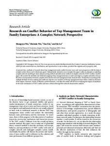
3and 5 MPa) were used while the variation of surfaces were recorded. Figure1 shows the shear
178
strength evolution under different normal loads. In this study, we focus on the patterns, obtained
179
from the test with a 3 MPa normal stress.
180
4. Implementation and Analysis of Complex Aperture Networks
181
In this section we set up the designated complex network over the aperture profiles,
182
which are perpendicular to the shear direction. By using the correlation measure, the distribution
183
of correlation values along profiles and during the successive shear displacements were obtained
184
(Fig.2). Plotting the correlation distribution shows the transition from a near Poisson distribution
185
to a Gaussian distribution. The change in the type of distribution is followed by the phenomena
186
of the tailing, which is inducing the homogeneity of the correlation values towards high and anti-
9
187
correlation values. In other words, tailing procedure is tied with the quasi-stable (residual part)
188
states of the joint. Thus, this can be described by reducing the entropy of the system where the
189
clusters of information over correlation space are formed. From another point of view, with
190
considering the correlation patterns, it can be inferred that throughout the shear procedure, there
191
is a relatively high correlation between each profile and the profiles at a certain neighborhood
192
radius. This radius of correlation is increasing non-uniformly (anisotropic development) during
193
shear displacement (Fig.3).
194
By using the method described in the previous section, a complex aperture network is
195
developed from the correlation patterns (Fig.4). As it can be seen in this figure, the formation of
196
highly correlated nodes (clusters) is distinguishable near the peak point. It can be estimated that
197
the controlling factor in the evolution path of the system is related to the formation of cliques
198
(communities). We will show locality properties of the clusters (intera structures) are much
199
more discriminated at last displacements rather than initial time steps while global variations of
200
the structures are more sensitive to reduction in the shear stress. In fact, forming hubs in the
201
constructed networks may give the key element of synchronization of aperture profiles (or
202
collective motion of discrete contact zones) along the shear process. In other words, reaching to
203
one or multiple attractors and the rate of this reaching after peak point are organized by the
204
spreading and stabilizing the clusters. Unfortunately, due to a low rate of data sampling, the
205
exact evolution of patterns before peak-point is not possible. However, during the discussion on
206
the joint degree correlations, a general concept will be proposed.
207
The three well-known characteristics of the constructed networks, namely total degree of
208
nodes, clustering coefficient and mean shortest path length are depicted as a function of shear
209
displacement in Figure 5.As it can be followed there is a nearly monotonic growth/decay of the 10
210
parameters. A considerable sharp change in transition from shear displacement 1 to 2 mm is
211
observed for all three illustrated parameters. This transition is assumed as state transition from
212
the pre-peak to post peak state, while with taking into account the rate of the variation of the
213
parameters the transformation step is discriminated. Also, despite of clustering coefficient trend
214
which show a fully-growth shape the number of edges and mean short length after a shear
215
displacement of 12 mm roughly exhibiting a quasi-stable trend. These results provide the
216
necessary information for the classification of the aperture networks in our rock joint. The high
217
clustering coefficient and low average (characteristic) path length clearly show that our aperture
218
networks have small-world properties.
219
The development of shear stress over the networks is much faster after the peak point
220
than the pre-peak states. This feature can be explained by understanding the concept of the net-
221
contact areas [59]. At interlocking of asperities step-before maximum static friction- the two-
222
point correlation shows a relatively more uniform shape rather than former and later cases. Also,
223
the current configuration implies that the homogeneity of the revealed network where the nodes
224
with high degree are tending to absorb nodes with low edges. This indicates the property of self-
225
similarity within the network structures. The shear displacements immediately after or near peak
226
(Figure 6) point destroy the homogeneity of the network and spreading slow fronts and dropping
227
of the frictional coefficient is accompanied with a trial to make stable cliques, inducing the
228
heterogeneity to the network structures. Using a microscopic analysis, it can be proven that, for
229
homogenous topologies, many small clusters spread over the network and merge together to
230
form a giant synchronized cluster [54-56]. This event is predicted before reaching to the peak
231
threshold. In heterogeneous graphs, however, one or more central cores (hubs) are driving the
232
evolutionary path and are figuring out the synchronization patterns by absorbing the small 11
233
clusters. As can be seen in Figure 6 and Figure 7, two giant groups are recognizable after 14 mm
234
displacement. This shows the attractors states in a dynamic system. However, two discriminated
235
clusters are not showing the self-similarity structures within the proper networks, i.e., hubs with
236
high degree nodes are separated from the hubs with low degree nodes. In general, one may
237
overestimate the self-similarity of internal structures of the networks, which means that in the
238
entire steps at least a small branch of fractility can be followed.
239
The attributed weight distribution, associated with the two-point correlation concept
240
(Fig.7) shows as if the virtual heaviness of edges are increasing, simultaneously, the joint degree
241
distribution is also growing, which indicates the networks are assortative. The distribution of the
242
weights from unveiled hubs also clearly can be followed in Figure 7 while two general
243
discriminated patterns are recognizable. On the contrary, if the patterns of correlation of
244
clustering coefficients are drawn (Fig.8), the eruption of local synchronization is generally closed
245
out after (or at least near) peak point while again during and after dropping shear strength, the
246
variation of local clusters will continue. Especially, at the point near to critical step, the local
247
clusters present much more uniform percolation rather than the other states while at final steps
248
the stable state (or quasi-stable) regime of regional structures is not clear. It is worth stressing the
249
rate of variation of local joint clustering patterns at apparently quasi-steps are much higher than
250
the global patterns, i.e., joint degree distribution. Also, it must be noticed that before peak point
251
the structures of joint triangles density is approximately unchangeable. Then as a conclusion,
252
burst of much dense local hubs is scaled with disclosing of slow fronts spreading.
253
Following the spectrum of the networks in a collective view (Fig.9) shows a nearly
254
uniform growing trend where a third degree polynomial may be fitted. However, with respect to
255
individual analysis (local analysis) of ci − k i , a negative trend can be pursued. The spectrum of 12
256
the networks can be related to three-point correlation concept which expresses the probability of
257
selecting a node with a certain degree, so that it is connected to other two nodes with the definite
258
degrees. The evolution of spectrum of aperture networks in a Euclidean space and using a
259
clustering analysis on the accumulated objects has come out the details of the fracture evolution,
260
either in the mechanical or hydro-mechanical analysis [18-19]. But, in our case, detecting such
261
explicit scaling is difficult. Let us transfer all of the calculated network properties in a variation
262
(rate) space (Fig.10). Depicting the clustering coefficient and mean degree rates, shows a similar
263
trend with the evolution of shear strength, however, after 8 mm displacement the variation of
264
edges and clustering coefficient unravels the different fluctuations.
The negative scaling (for large anisotropy) in
265
dci dki − space can be expressed by dt dt
266
dki dc ≅ −800 i + 20 . As it can be followed in Figure 10, the congestion of objects makes a dt dt
267
general elliptic which approximately covers all of points where the details of the correlation
268
among two components presents how the expansion and contraction of patterns fall into the final
269
attractors (Fig.10). Thus, such emerged patterns related to the two-point correlation of variation
270
rate of edges and rate of clustering coefficient are proposing a certain core in each time step so
271
that the absorbing of objects within a “black hole” at residual part is much more obvious rather
σ(
d≺k ) dt
272
than other states. With definition of anisotropy by S =
273
deviation), the rate changes of profiles in a new space and with reference to the pre and post peak
274
behaviours are obtained (Fig.11). Transferring from interlocking step to Coulomb threshold level
275
is accompanying with the maximum anisotropy (Fig.11b) and immediate dropping and then
13
dC ( σ is standard σ( ) dt
276
starting to fluctuate until reaching to a uniform decline. The fluctuation of anisotropy from 2mm
277
to 13 mm may be associated with the stick-slip behaviour of the rock joint as the main reason of
278
shallow earthquakes [57-58]. It should be noticed that the results of the later new space is
279
completely matching with the analysis of joint degree and joint clustering distribution. In Figure
280
11.a, we have illustrated a new variable with regard to durability and entropy of the system,
281
dC d ≺ k × dt dt
282
while initiating the post stick-slip behavior is scaled with the minus or zero variation of the
283
parameter. In [59-61], we analyzed the sub-graph structures and frequencies over parallel and
284
perpendicular aperture networks. Also, a directed network based on contact strings and
285
preferentiality of possible energy flow in rupture tips has been introduced. We also, inspected the
286
synchronization of strings using a Kuromoto model [59].
. In fact with definition of such parameter the fluctuation in anisotropy is filtered
5. Conclusions
287 288
In this study, we presented a special type of complex aperture network based on
289
correlation measures. The main purpose of the study was to make a connection between the
290
apparent mechanical behavior of a rock joint and the characterized network. The incorporation of
291
the correlation of apertures and the evaluation of continuously changing contact areas (i.e.
292
growth of aperture) within the networks showed the effects of structural complexity on the
293
evolution path of a rock joint. Our results showed that the main characteristics of aperture
294
networks are related to the shear strength behavior of a rock joint. The residual shear strength
295
corresponded to the formation of giant groups of nodes in the networks. In addition, based on the
296
joint correlation upon edges and triangles, the pre-peak and post peak behaviour of a rock joint
297
under shear were analyzed. Our results may be used as an approach to insert the complex 14
298
aperture networks into the surface growth methods or general understanding of the conditions for
299
a sudden movement (shock) in a fault.
300 301
References
302 303 304 305 306 307 308 309 310 311 312 313 314 315 316 317
1. Newman M. E. J. The structure and function of complex networks, SIAM Review 2003; 45(2): 167- 256.
318 319 320 321 322 323 324 325 326 327 328 329 330
6. Baiesi M, Paczuski M. 2004.Scale free networks of earthquakes and aftershocks. Physical review E 2004; 69 (2): 066106.1-066106.8
331 332 333 334 335 336
10. Xie F, Levinson D. Topological evolution of surface transportation networks. Computers, Environment and Urban Systems 33 (2009) 211–223
2. Dorogovetev S.N., Goltsev A.V.2008.Critical phenomena in complex networks .Review Modern Physics.Vol.80.Oct-Dec.2008 3. Boccaletti S.,Latora V., Moreno Y.,Chavez M.,Hwang D-U.2006.Complex Networks : Structure and Dynamics. Physics Reports 424,175-308 4. Abe S, Suzuki N.2006. Geophys;13:145-150
Complex network description of seismicity. Nonlin process
5. Jim´enez A, Tiampo K.F., Posadas A.M., Luz´on F., and Donner R. Analysis of complex networks associated to seismic clusters near the Itoiz reservoir dam. Eur. Phys. J. Special Topics 2009; 174, 181–195.
7. Doering R.C.1991.Modeling Complex Systems: Stochastic processes, Stochastic Differential Equations, and Fokker-Planck Equations; 1990 Lectures in complex systems, SFI Studies in the science of complexity. 8. Ghaffari H.O., Sharifzadeh M Shahriar , K. & Pedrycz W. Application of soft granulation theory to permeability analysis , International Journal of Rock Mechanics and Mining Sciences, Volume 46, Issue 3, 2009, Pages 577-589 9. Tsonis, A. A., and P. J. Roebber. 2003. The architecture of the climate network. Physica, 333A, 497–504.
11. Tsonis, A.A. and Swanson, K. L.2008. Topology and Predictability of El Nin˜o and La Nin˜a Networks. Physical Review Letters 100, 228502 (2008)
15
337 338 339 340
12. Bartolo1 S.D, Dell’Accio F, and Veltri M.2009. Approximations on the Peano river network: Application of the Horton-Strahler hierarchy to the case of low connections, Phys. Rev. E 79, 026108 (2009).
341 342 343
13. Latora V., Marchiori M. 2002, Is the Boston subway a small-world network? Physica A, 314, 109-113.
344 345 346 347 348 349 350 351 352 353 354 355 356 357 358 359 360 361 362
14. Mooney S.J, Dean K. Using complex networks to model 2-D and 3-D soil porous architecture. Soil Sci Soc Am J 73:1094-1100 (2009)
363 364 365
20. Walker D.M, Tordesillas A. Topological evolution in dense granular materials: a complex networks perspective. International Journal of Solids and Structures 47, 2010, 624-639.
366 367 368
21. Albert R., Barabasi A.-L. Statistical mechanics of complex networks. Review of Modern Physics; 74,2002, 47–97.
369 370 371 372 373 374 375 376 377
22. Alkan H. Percolation model for dilatancy-induced permeability of the excavation damaged zone in rock salt, International Journal of Rock Mechanics and Mining Sciences, 46(4), 2009, Pages 716-724.
15. Perez-Reche F, Taraskin S.N, Neri F.M, Gilligan C.A.2009.Biological invasion in soil :complex network analysis . Proceedings of the 16th international conference on Digital Signal Processing, Santorin, Greece .2009. 16. Karabacak T, Guclu H, Yuksel M. Network behaviour in thin film growth dynamics. Phys. Rev. B 79, 195418 (2009) – Published May 15, 2009 17. Valentini L Perugini D, Poli G. The small-world topology of rock fracture networks. Physica A 2007; 377:323–328. 18. Ghaffari H.O., Sharifzadeh M. & Fall M. Analysis of Aperture Evolution in a Rock Joint Using a Complex Network Approach; International Journal of Rock Mechanics and Mining Sciences, Volume 47, Issue 1, January 2010, Pages 17-29. 19. Ghaffari H.O., Sharifzadeh M. http://aps.arxiv.org/abs/0901.4413
.,Evgin
E;
Complex
Aperture
Networks.
23. Adler MP and Thovert JF. Fractures and fracture networks. Kluwer Academic; 1999. 24. Alava M. J , Nukala P.K. V. V.; Zapperi S, Statistical models of fracture , Advances in Physics, Volume 55, Issue 3 , 2006 , pages 349 – 476.
16
378 379 380
25. Knopoff, L. The organization of seismicity on fault networks, PNAS April 30, 1996 vol. 93 no. 9 3830-3837.
381 382 383
26. R.W. Zimmerman, D.W. Chen and N.G.W. Cook, The effect of contact area on the permeability of fractures, J Hydrol 139 (1992), pp. 79–96.
384 385 386 387 388 389 390 391 392 393 394 395 396 397 398
27. Lanaro F.A. Random field model for surface roughness and aperture of rock fractures. Int J Rock Mech Min Sci, 2000, 37:1195-1210.
399
32. Wilson RJ. Introduction to Graph Theory. Fourth Edition: Prentice Hall, Harlow, 1996.
400 401 402 403 404 405 406 407
33. Gao Z. and Jin N. Flow-pattern identification and nonlinear dynamics of gas-liquid twophase flow in complex networks; 2009.Physical Review E 79, 066303.
408 409 410
36. Colizza, V., Flammini, A., Serrano, M.A., Vespignani, A. Detecting rich-club ordering in complex networks, Nature Physics 2, Issue 2, 2006, Pages 110-115 .
411 412 413
37. Song C, Havlin S, Makse HA., Origins of fractality in the growth of complex networks, Nature Physics 2, 275 - 281 (2006), pages 275-281.
414 415 416
38. Kim JS, Goh KI, Salvi G, Oh E, Kahng B, Kim D, Fractality in complex networks: Critical and supercritical skeletons, Phys. Rev. E 75, 016110 (2007).
28. Brown SR, Kranz RL , Bonner BP. Correlation between the surfaces of natural rock joints, Geophys Res Lett, 1986; 13(13):1430-1433. 29. Hakami E, Einstein H H,Genitier S , Iwano M. Characterization of fracture aperturesmethods and parameters. In: Proc of the 8th Int Congr on Rock Mech, Tokyo, 1995: 751-754. 30. Lanaro F, Stephansson O.A. Unified model for characterization and mechanical behavior of rock fractures. Pure Appl Geophys,2003;160:989-998 31. Ghaffari H. O, Complexity Analysis of Unsaturated Flow in Heterogeneous Media Using a Complex Network Approach, http://arxiv.org/ftp/arxiv/papers/0912/0912.4991.pdf
34. Newman M.E.J. Assortative mixing in networks. Phys. Rev. Lett. 89, 208701 (2002). 35. R. Xulvi-Brunet and I.M. Sokolov. Changing correlations in networks: assortativity and dissortativity. Acta Phys. Pol. B, 36, 1431 (2005).
17
417 418 419 420
39. Korniss G, Synchronization in weighted uncorrelated complex networks in a noisy environment: Optimization and connections with transport efficiency, Phys. Rev. E 75, 051121 (2007).
421 422 423
40. Dijkstra EW, A note on two problems in connexion with graphs, Numerische mathematik, 1959 ,pp. 269-271.Springer
424 425 426
41. Newman M., Barabasi A-L., Watts D.J.The Structure and Dynamics of Networks.2006. Princeton University Press
427 428 429
42. Watts DJ, Strogatz SH. Collective dynamics of small-world networks. Nature ,1998; 393:440-442
430 431 432 433
43. Mitani, Y., Esaki, T., Zhou, G., Nakashima, Y. Experiments and simulation of Shear – Flow Coupling properties of rock joint. In: Proc., 39th Rock mechanics conference: Glückauf, Essen, (2003), 1459–1464.
434 435 436 437
44. Mitani, Y., Esaki, T., Sharifzadeh, M., Vallier, F. Shear – Flow coupling properties of rock joint and its modeling Geographical Information System (GIS). In: Proc., 10th ISRM Conference, South African Institute of Mining and Metallurgy, (2003), 829–832.
438 439 440 441 442 443 444
45. Sharifzadeh M. Experimental and theoretical research on hydro-mechanical coupling properties of rock joint. Ph.D. thesis, Kyushu University, Japan; 2005.
445 446 447 448 449
47. L. Valentini, D. Perugini and G. Poli, The ‘small-world’ nature of fracture/conduit networks:next term Possible implications for disequilibrium transport of magmas beneath mid-ocean ridges, Journal of Volcanology and Geothermal Research 159 (2007), pp. 355– 365.
450 451
48. Gnecco, Enrico; Meyer, Ernst, Fundamentals of Friction and Wear, 2007, Springer, 714 p.
452 453 454
49. Rubinstein, S., Cohen, G. & Fineberg, J. Contact area measurements reveal loading-history dependence of static friction. Phys. Rev. Lett. 96, 256103 (2006)
46. Sharifzadeh M, Mitani Y, Esaki T .Rock joint surfaces measurement and analysis of aperture distribution under different normal and shear loading using GIS, Rock Mechanics and Rock Engineering, Volume 41, Number 2 / April, 2008, Pages 299-323.
18
455 456 457
50. Xia, K., Rosakis, A. J. & Kanamori, H. Laboratory earthquakes: the sub-Raleigh-tosupershear rupture transition. Science 303, 1859–1861 (2004)
458 459 460
51. Rubinstein, S. M., Cohen, G. & Fineberg, J. Detachment fronts and the onset of dynamic friction. Nature 430, 1005–1009 (2004)
461 462 463 464
52. S. M. Rubinstein, G. Cohen, and J. Fineberg, Visualizing Stick-Slip: Experimental observations of processes governing the nucleation of frictional sliding, J. Phys. D: Appl. Phys. 42 214016, (2009).
465 466 467
53. Sornette D, Critical Phenomena in Natural Sciences, Springer-Verlag Berlin Heidelberg, 2006.
468 469 470
54. Arenas A., Diaz-Guilera A., Kurths J., Moreno Y., Zhou C. Synchronization in complex networks .Physics Reports ,2008, 469,93-153.
471 472 473 474 475
55. Strogatz,S.H. Exploring complex networks, Nature. 2001; Vol .410:268-276.
476 477 478
57. Brace WF, Byerlee JD, Stick-slip as a mechanism for earthquakes, Science, Volume 153, Issue 3739, pp. 990-992.
479 480
58. Scholz CH, Earthquakes and friction laws, Nature, 391, 37-42 (1998).
481 482
59. H.O.Ghaffari and R.P.Young, ArXive-prints (2011) http://arxiv.org/abs/1105.4265.
483 484
60. H.O.Ghaffari, A.Nabovati, M. Sharifzadeh, and R.P.Young, http://arxiv.org/abs/1103.1124.
485 486
61. H.O.Ghaffari and R.P.Young, Motifs of Networks from Shear Fractures; submitted to Journal
56. Barahona M, and Pecora L. M. Synchronization in Small-World Systems, Phys. Rev. Lett. 89, 054101 (2002)
487 488 489 19
490 491 492 493 494 495 496 497
Figures
498
499
20
case1 case3 case5 case6
8 7
SS(MPa)
6 5 4 3 2 1 0 0
500
2
4
6
8
10
12
14
16
18
20
SD(mm)
501
FIGURE 1. Variation of shear strength for different cases (normal stresses for
502
case1:1mpa, case3: 3 MPa, case5: 5 MPa and case6: 3 MPa (without control of upper
503
shear box) [46].
504 505 506 507 508
21
509 510
FIGURE 2. Evolution of correlation values of aperture profiles at shear displacement s:
511
0,2,10 and 20 mm.
512
22
900 800
SD=0
800 700
700
600
600
600
500
500
500
400
400
400
300
300
300
200
200
200 100
800
200
300
400
500
600
700
800
900
1
SD=4
0.8 0.6
100 100
0.4 0.2
100 100
200
300
400
500
600
700
800
100
200
300
400
500
600
700
800
0
800
SD=5
800
700
SD=10
700
-0.2
SD=20
700
600
600
-0.4
600
500
500
500
400
200 100
200
513
400
600
-0.6
400
400
300
514
800
SD=2
700
300
300
200
200
100
100
-0.8 -1
800
200
400
600
800
200
400
600
800
FIGURE 3. Correlation patterns throughout the shear displacements 900 800
800
SD=0
800
SD=2
700
700
700
600
600
600
500
500
500
400
400
400
300
300
300
200
200
200
100
100
100
200
400
600
0.9
100
800
1
SD=5
200
300
400
500
600
700
800
0.8 0.7 0.6 100
200
300
400
500
600
700
800
0.5 800
800 700
800
SD=10
700
600
515 516
SD=15
700
500
500
500
400
400
400
300
300
300
200
200
200
100
100
100
200
300
400
500
600
700
800
0.3
600
600
100
0.2 0.1
0 100
200
300
400
500
600
700
800
100
200
FIGURE 4. Visualization of adjacency matrix for the achieved networks 23
0.4
SD=20
300
400
500
600
700
800
0
K
C
0.7
11
a)
0.65
4
x 10
2.25
b)
10
c)
2.2 2.15
9
0.6
mean geodesic distance
2.1 8
K
C
0.55
7
0.5
6
2.05 2 1.95 1.9
0.45
5
1.85 0.4
0.35
517
4
0
2
4
6
8
10 SD(mm)
12
14
16
18
3
20
1.8 1.75 0
2
4
6
8
10 SD(mm)
12
14
16
18
20
0
2
4
6
8
10 SD(mm)
12
14
518
FIGURE 5. a) Clustering coefficient-Shear Displacement (SD), b) Number of edges-SD
519
and c) Average path length-SD ρ ( ki , k j ) SD=0mm
SD=1mm 250
20 18
250
16
200
12
150
150
12
10
16
150
12 10
10
100
8
100
8
6
6
200
16
150
12
50
4
50
4
150
12
10
10 100
8
100
8
200
6
50
4
50
4
50
6 50
4 2
2
Number of Bins(kj)
14
12
100
8
2 2
4
6
8
10
12
14
16
18
20
2
2
0
2
4
6
8
10
12
14
16
18
0
20
2
4
6
8
SD=8mm
SD=7mm 250
20
10
12
14
16
18
0
20
2 2
4
6
8
10
12
14
16
18
0
20
5
SD=9
250
20
250
20
200
16
200
16
150
12
150
12
150
10
10 100
8
100
8
6
100
8
14 12
10 SD=14mm
15
20
0 SD=15mm 10
5 250
15
20
0
5
10 SD=16mm
250
20
15
20
100
8
50
4
4
6
8
10
12
14
16
18
20
250
20
200
16
200
16
18
150
12
150
12
14
250
20
100
8 6
50
4
50
4
5
10
15
20
0
2
4
6
8
10
12
14
16
18
20
0
250
200
10 SD=18mm
15
6
18
10 SD=19mm
15
0
20
10
15
0
20
SD=20mm 250
20
200
16
18 200
16
14 150
5
250
20 18
200
150
12
50
14 150
12
10
100
2
5 250
50
4
0
20
100
8
10 100
8
100
8
10 100
8
100
6
6 6
6
6
15
20
50
2 5
0
5
10
15
20
0
50
4
2
2 10
4
50
4
5
50
4
50
2
10
15
20
0
2
5
10
15
20
0 2
4
6
8
10
12
14
16
18
20
0
Number of Bins(ki)
521
FIGURE 6. Joint degree distribution from SD=0 to SD=20 mm (Top left-first row is
522
SD=0 and Top right -first row is 6mm shear slip )
24
150
150
50
2
150
8
4
2
2
SD=13mm
10 100
4
12
100
8 6
12
6
5
10
0
20
14 150
8
14
12
10
15
18 200
16
50
4
16
150
12 100
8
10
250
20
200
16 14
10
10
8
20
18 200
16 14
14
20
12
0
SD=17
18
18
18
10
2
2
0
16
100
2
2 5
14
14 150
150
12
2
20
12
16
6
50
4
10
20
6
50
4
8
18 200
10
6
6 50
4
6
SD=12mm 250
16
10 10
4
5
18
14
12
2
0
20
200
16
14
14
14
15
2
0
250
18
200
16
10 SD=11mm
20
SD=10mm 20
18
18
18
2
520
200
16
150
6
4
250
18
16
50
4
250
20
200
14
10 100
8 6
6
250
20 18
14
100
8
SD=6mm
SD=5mm
250
20 18
200
14
14
12
10
200
16
14 150
250
20 18
18
16
14
250
20
18
SD=4mm
SD=3mm
SD=2mm
20
200
0
16
18
20
ρ (ki + k j / 2) SD=1mm
SD=0mm
SD=2mm
350
500
SD=3mm
450
450
700
400
300
600
400
350 250
350
500 300
300
200
400
250
250 200
150
300
200 150
100
150
200 100
100 50
0
100
50
50
0
50
100
150
200
250
0 20
40
60
80
100
SD=4mm
140
160
180
200
220
0
0
50
100
SD=10mm
700
1400
600
1200
500
1000
400
150
200
250
0
0
50
100
SD=15mm
150
200
250
300
300
350
400
SD=20mm
1200
1200
1000
1000
800
800
600
600
400
400
800
300
600
200
400
100
200
0 50
120
100
150
200
250
300
0 100
200
150
200
250
300
350
0 100
200
150
200
250
300
350
400
0 100
150
200
250
(ki)+(ki)/2
523 524
FIGURE 7. Attributed weight distribution of links related to joint degree distribution
525
(for SD=0-4,10,15 and 20 mm)
25
ρ (ci , c j )
500
SD=0mm
SD=1mm
SD=4mm
SD=3mm
SD=2mm
SD=5mm
20
20
20
20
20
20
18
18
18
18
18
18
18
16
16
16
16
16
16
14
14
14
14
14
14
12
12
12
12
12
10
10
10
10
10
8
8
8
8
6
6
6
6
4
4
4
4
2
2
2
2
16 14 12 10
450
SD=6mm
20
8 6 4 2 2
4
6
8
10
12
14
16
18
20
2
600
4
6
8
10
12
14
16
18
20
2
4
6
8
10
12
14
16
18
20
2
4
6
8
10
12
14
16
18
12 10
8
8
6
6
4
4 2 2
20
4
6
8
10
12
14
16
18
2
20
2
600
700
600
700
4
6
8
10
12
14
16
18
20
2
800
4
6
8
10
12
14
16
18
20
900
400
600
500
500
500 500
400
400
400
300
300
200
200
700
600
500
400
400
300 300
800
600
700
500
600
400
500
300 200 200
400
300 200
350
100
100
0 0.2
0.25
0.3
0.35
0.4
0.45
0.5
0.55
0.6
0 0.2
0.65
0.25
0.3
0.35
0.4
0.45
0.5
0.55
0.6
300
200
100
100
200
100
100
0.65
0 0.25
0.3
0.35
0.4
0.45
0.5
0.55
0.6
0.65
100
0
0.35
0.4
0.45
0.5
0.55
0.6
0.65
0.7
0 0.35
0.4
0.45
0.5
0.55
0.6
0.65
0.7
0.75 0 0.4
0.45
0.5
0.55
0.6
0.65
0.7
0.75
0 0.4
SD=7mm SD=8mm
20 20
18
300
12 10 8 6
250
10
12
14
16
18
18
16
16
16
14
14
14
12
12
10
10
8
8
6
6
4
4
2
2
10
8
8
8
6
6
6
4
4
2
2
2
4
6
8
10
12
14
16
18
12 10
900
700
800
6
8
10
12
14
16
18
20
2
1000
4
6
8
10
12
14
16
18
1200
600
14
16
18
8 6 4
20
2
4
6
8
10
12
14
16
18
2
20
2
1200
300
0.45
0.5
0.55
800
800
600
600
400
400
0.6
0.65
0.7
0.75
0.5
0.55
0.6
200
200
0.65
0.7
0.75
0.8
SD=15mm
0.5
0.55
0.6
0.65
0.7
0.75
0.8
0 0.4
0.45
0.5
0.55
0.6
0.65
0.7
0.75
300
0.5
0.55
0.6
0.65
0.7
0 0.45
0.75
0.5
0.55
0.6
0.65
SD=18mm
0.7
0.75
0 0.45
0.8
SD=19mm
16
16
14
14
12
12
10
10
10
8 6 4 2 2
4
6
8
10
12
14
16
18
20
20
18
18
18
0.55
0.6
16
16
16
14
14
14
12
12
12
12
10
10
10
10
8
8
8
6
6
6
6
6
6
4
4
4
4
4
2
2
2
2
2
2
4
6
8
10 12 SD=15mm
14
16
18
20
2000
1800
1800
1600
6
8
10
12
14
16
18
20
2
4
6
8
10
12
14
16
18
20
2
1600
1200
1400
1600
600
0.65
0.7
0.75
0.8
0.85
0.9
12
14
16
18
20
4 2 2
1400
1400
1200
1200
4
6
8
10
12
14
16
18
20
2
4
6
8
10
12
14
16
18
20
0.85
0.9
0.95
1800 1600
1000
1000
800
800
1000
600
600
800
400
400
200
200
1200
600
600
600
400
0.6
10
800
800 800
0.55
8
1000
1000 1000
400
400
400
200
200
200
0 0.45
6
1400
1200 1200
200
4
1200
800
600
0.8
1400
1400
1000
0.75
14
8
4
0.7
16
8
2
0.65
18
8
20
1400
0 0.5
0.5
20
20
18
12
20
SD=20mm
20
14
18
200
0 0.45
0.8
SD=17mm
18
16
16
100
0 0.45
20
18
14
400
SD=16mm
20
12
500
400
100
SD=14mm
10
700 600
200
0 0.45
8
800
200 100
6
1000
600
400
200
4
1000
800
500
300
0 0.4
526
12
1000
200
0
10
1000
400 300
100
50
8
700
400
0.75
900
500
100
6
1200
600
150
4
900
500
0.7
10
20
1400
700
200
0.65
12
2
4
800 600
0.6
SD=13mm
14
20
2 800
0.55
16
12
20
0.5
18
14
2
8
18
10
4
6
18
12
2 4
20
14
4
2
20
20
16
16
14
0.45
SD=12mm
20
18
18
16
SD=11mm
SD=10mm
20
400
0.5
0.55
0.6
0.65
0.7
0.75
0.8
0.85
0.9
0 0.4
0.45
0.5
0.55
0.6
0.65
0.7
0.75
0.8
0 0.4
0.45
0.5
0.55
0.6
0.65
0.7
0.75
0.8
0.85
0.9
0 0.45
0.5
0.55
0.6
0.65
0.7
0.75
0.8
0.85
0 0.9 0.5
200
0.55
0.6
0.65
0.7
0.75
0.8
0.85
0 0.90.5
0.55
0.6
0.65
0.7
0.75
0.8
527
FIGURE 8. Joint clustering coefficient distribution plus attributed weight histograms
528
based on averages of triangles connected to a link (sequence of figures are as well as
529
figure 6).
530 531
26
140
≺ K
data1
-0.1
10
data2
a)
3
data3 data4
120
2
y = - 5.2e+003*x + 7.6e+003*x - 3.3e+003*x + 4.9e+002 data fit
data5 -0.2
b)
data6
10
data7 data8
100
data9 data10
-0.3
10
data11
1/N*
ci
data12 ci
data13 data14
-0.4
10
data15
80
data16 data17
60
data18 -0.5
10
data19 data20
40
-0.6
10
ki
-0.7
10
532
1
20 0.35
2
10
C 0.4
0.45
0.5
10 ki
0.55
0.6
0.65
3
10
533
FIGURE 9. a) Spectrum of complex aperture networks ( ci - ki )and b) Evolution of mean
534
degree of node against clustering coefficient and fitness of a polynomial function
535 536
120
100
80
dki dt
data1 data2 data3 data4 data5 data6 data7 data8 data9 data10 data11 data12 data13 data14 data15 data16 data17 data18 data19 data20
60
i
dk /dt
40
20
0
-20
-40
-60
-80 -0.15
-0.1
-0.05
0
0.05 dc i/dt
537
0.1
dci dt
0.2
dki dci − space with respect to shear displacements dt dt
538
FIGURE 10. Data accumulation in
539
(data1to data 20 are related to shear displacements from 0 to20 mm ).
27
0.15
0.7
540
dC d ≺ k × dt dt
S=
0.9
σ(
d≺k dt
)
σ(
560
a)
0.8
dC ) dt
b)
540 0.7
520 0.6
STD(dk/dt)/STD(dc/dt)
500
d < k > /d t*d c /d t
0.5
0.4
0.3
480
460
440 0.2
420 0.1
400 0
-0.1
380 0
1
2
3
4
5
6
7
8
9
10 SD(mm)
11
12
13
14
15
16
17
18
19
20
0
sd (m m )
541
2
3
4
5
6
7
8
9
10 11 SD(mm)
12
13
14
15
16
17
sd (m m )
dC d < k > × with shear displacements and b) Anisotropy dt dt
542
FIGURE 11.a) Variation of
543
evolution at the rate of spectrum (networks) space
544
28
1
18
19
20