Component Specification for Parallel Coupling Infrastructure

Component Specification for Parallel Coupling Infrastructure J. Walter Larson1,2 and Boyana Norris1 1

Mathematics and Computer Science Division, Argonne National Laboratory, Argonne, IL 60439, USA {larson,norris}@mcs.anl.gov 2 ANU Supercomputer Facility, The Australian National University, Canberra ACT 0200 Australia

Abstract. Coupled systems comprise multiple mutually interacting subsystems, and are an increasingly common computational science application, most notably as multiscale and multiphysics models. Parallel computing, and in particular message-passing programming have spurred the development of these models, but also present a parallel coupling problem (PCP) in the form of intermodel data dependencies. The PCP complicates model coupling through requirements for the description, transfer, and transformation of the distributed data that models in a parallel coupled system exchange. Component-based software engineering has been proposed as one means of conquering software complexity in scientific applications, and given the compound nature of coupled models, it is a natural approach to addressing the parallel coupling problem. We define a software component specification for solving the parallel coupling problem. This design draws from the already successful Common Component Architecture (CCA). We abstract the parallel coupling problem’s elements and map them onto a set of CCA components, defining a parallel coupling infrastructure toolkit. We discuss a reference implementation based on the Model Coupling Toolkit. We demonstrate how these components might be deployed to solve a relevant coupling problems in climate modeling.

1

Introduction

Multiphysics and multiscale models share one salient algorithmic feature: They involve interactions between distinct models for different physical phenomena. Multiphysics systems entail coupling of distinct interacting natural phenomena; a classic example is a coupled climate model, involving interactions between the Earth’s atmosphere, ocean, cryosphere, and biosphere. Multiscale systems bridge distinct and interacting spatiotemporal scales; a good example can be found in numerical weather prediction, where models typically solve the atmosphere’s primitive equations on multiple nested and interacting spatial domains. These systems are more generally labeled as coupled systems, and the set of interactions between their constituent parts are called couplings. O. Gervasi and M. Gavrilova (Eds.): ICCSA 2007, LNCS 4707, Part III, pp. 55–68, 2007. c Springer-Verlag Berlin Heidelberg 2007

56

J.W. Larson and B. Norris

Though the first coupled climate model was created over 30 years ago [1], their proliferation has been dramatic in the past decade as a result of increased computing power. On a computer platform with a single address space, coupling introduces algorithmic complexity by requiring data transformation such as integrid interpolation or time accumulation through averaging of state variables or integration of interfacial fluxes. On a distributed-memory platform, however, the lack of a global address space adds further algorithmic complexity. Since distributed data are exchanged between the coupled model’s constituent subsystems, their description must include a domain decomposition. If domain decompositions differ for data on source and target subsystems, the data traffic between them involves a communication schedule to route the data from source to destination. Furthermore, all data processing associated with data transformation will in principle involve explicit parallelism. The resultant situation is called the parallel coupling problem (PCP) [2, 3]. Myriad application-specific solutions to the PCP have been developed [4, 5, 6, 7,8,9,10]. Some packages address portions of the PCP (e.g., the M×N problem— see [11]). Fewer attempts have been made to devise a flexible and more comprehensive solution [2,12]. We propose here the development of a parallel coupling infrastructure toolkit, PCI-Tk, based on the component-based software engineering strategy defined by the Common Component Architecture Forum. We present a component specification for coupling, an implementation based on the Model Coupling Toolkit [2, 13, 14], and climate modeling as an example application.

2

The Parallel Coupling Problem

We begin with an overview of the PCP. For a full discussion readers should consult Refs. [2, 3]. 2.1

Coupled Systems

A coupled system M comprises a set of N subsystem models called constituents {C1 , . . . , CN }. Each constituent Ci solves its equations of evolution for a set of state variables φi , using a set of input variables αi , and producing a set of output variables βi . Each constituent Ci has a spatial domain Γi ; its boundary ∂Γi is the portion Γi exposed to other models for coupling. The state Ui of Ci is the Cartesian product of the set of state variables φi and the domain Γi , that is, Ui ≡ φi × Γi . The state Ui of Ci is computed from its current value and a set of coupling inputs Vi ≡ αi × ∂Γi from one or more other constituents in {C1 , . . . , CN }. Coupling outputs Wi ≡ βi × ∂Γi are computed by Ci for use by one or more other constituents in {C1 , . . . , CN }. Coupling between between constituents Ci and Cj occurs if the following conditions hold: 1. Their computational domains overlap, that is, the coupling overlap domain Ωij ≡ Γi ∩ Γj = ∅. 2. They coincide in time.

Component Specification for Parallel Coupling Infrastructure

57

3. Outputs from one constituent serve as inputs to the other, specifically (a) Wj ∩Vi = ∅ and/or Vj ∩Wi = ∅ or (b) the inputs Vi (Vj ) can be computed from the outputs Wj (Wi ). In practice, the constituents are numerical models, and both Γi and ∂Γi are ˆ i (·), resulting in meshes D ˆ i (Γi ) and discretized1 by the discretization operator D ˆ i (∂Γi ), respectively. Discretization of the domains Γi leads to definitions of D ˆ i of state, input, and output vectors for each constituent Ci : The state vector U Ci is the Cartesian product of the state variables φi and the discretization of ˆ i ≡ φi × D ˆ i (Γi ). The input and output vectors of Ci are defined as Γi ; that is, U ˆ ˆ ˆ i ≡ βi × D ˆ i (∂Γi ), respectively. Vi ≡ αi × Di (∂Γi ) and W The types of couplings in M can be classified as diagnostic or prognostic, explicit or implict. Consider coupling between Ci and Cj in which Ci receives among its inputs data from outputs of Cj . Diagnostic coupling occurs if the outputs Wj used as input to Ci are computed a posteriori from the state Uj . Prognostic coupling occurs if the outputs Wj used as input to Ci are computed as a forecast based on the state Uj . Explicit coupling occurs if there is no overlap in space and time between the states Ui and Uj . Implicit coupling occurs if there is overlap in space and time between Ui and Uj , requiring a simultaneous, self-consistent solution for Ui and Uj . Consider explicit coupling in which Ci receives input from Cj . The input state ˆ i is computed from a coupling transformation Tji : W ˆj → V ˆ i . The vector V coupling transformation Tji is a composition of two transformations: a mesh ˆ j (Ωij ) → D ˆ i (Ωij ) and a field variable transformation transformation Gji : D Fji : βj → αi . Intergrid interpolation, often cast as a linear transformation, is a simple example of Gji , but Gji can be more general, such as a spectral transformation or a transformation betweeen Eulerian and Lagrangian representations. The variable transformation Fji is application-specific, defined by the natural law relationships between βj and αi . In general, Gji ◦ Fji = Fji ◦ Gji ; that is, the choice of operation order Gji ◦ Fji versus Fji ◦ Gji is up to the coupled model developer and is a source of coupled model uncertainty. A coupled model M can be represented as a directed graph G in which the constituents are nodes and their data dependencies are directed edges. The connectivity of M is expressible in terms of the nonzero elements of the adjacency matrix A of G. For a constituent’s associated node, the number of incoming and outgoing edges corresponds to the number of couplings. If a node has only incoming (outgoing) edges, it is a sink (source) on G, and this model may in principle be run off-line, using (providing) time history output (input) from (to) the rest of the coupled system. In some cases, a node may have two or more incoming edges, which may require merging of multiple outputs for use as input data. For a constituent Ci with incoming edges directed from Cj and Ck , merging ˆ i if the following conditions hold: of data will be required to create V 1

We will use the terms “mesh,” “grid,” “mesh points,” and “grid points” interchangeably with the term “spatial discretization.”

58


1. The constituents Ci , Cj , and Ck coincide in time. 2. The coupling domains Ωij and Ωik overlap, resulting in a merge domain Ωijk ≡ Ωij ∩ Ωik = ∅. 3. Shared variables exist among the fields delivered from Cj and Ck to Ci , namely, (βj ∩ αi ) ∩ (βk ∩ αi ) = ∅. The time evolution of the coupled system is marked by coupling events, which either can occur predictibly following a schedule or can be threshhold-triggered based on some condition satisfied by the constituents’ states. In some cases, the set of coupling events fall into a repeatable periodic schedule called a coupling cycle. For explicit coupling in which Ci depends on Cj for input, the time sampling ˆ j or as of the output from Cj can come in the form of instantaneous values of W ˆ a time integral of Wj , the latter used in some coupled climate models [15, 6]. 2.2

Consequences of Distributed-Memory Parallelism

The discussion of coupling thus far is equally applicable to a single global address space or a distributed-memory parallel system. Developers of parallel coupled models confront numerous parallel programming challenges within the PCP. These challenges fall into two categories. Coupled model architecture encompasses the layout and allocation of the coupled model’s resources and execution scheduling of its constituents. Parallel data processing is the set of operations necessary to accomplish data interplay between the constituents. On distributed-memory platforms, the coupled-model developer faces a strategic decision regarding the mapping of the constituents to processors and the scheduling of their execution. Two main strategies exist—serial and parallel composition [16]. In a serial composition, all of the processors available are kept in a single pool, and the system’s constituents each execute in turn using all of the processors available. In a parallel composition the set of available processors is divided into N disjoint groups called cohorts, and the constituents execute simultaneously, each on its own cohort. Serial composition has a simple conceptual design but can be a poor choice if the constituents do not have roughly the same parallel scalability; moreover, it restricts the model implementation to a single executable. Parallel composition offers the developer the option of sizing the cohorts based on their respective constituents’ scalability; moreover, it enables the coupled model to be implemented as multiple executables. The chief disadvantage is that the concurrently executing constituents may be forced to wait for input data, causing cascading, hard-to-predict, and hard-to-control execution delays, which can complicate the coupled model’s load balance. A third strategy, called hybrid composition, involves nesting one within the other to one or more levels (e.g., serial within parallel or vice versa). A fourth strategy, called overlapping composition, involves dividing the processor pool such that the constituents share some of the processors in their respective cohorts; this approach may be useful in implementing implicit coupling.


59

In a single global address space, description and transfer of coupling data are straightforward, and exchanges can be as simple as passing arguments through function interfaces. Standards for field data description (i.e., the αi and βi ) and mesh description for the coupling overlap domains Ωij (i.e., their discretizations ˆ i (Ωij )) are sufficient. Distributed memory requires additional data descripD tion in the form of a domain decomposition Pi (·), which splits the coupling ˆ i and ˆ i (Ωij ) and associated input and output vectors V overlap domain mesh D ˆ i into their respective local components across the processes {p1 , p2 , . . . , pKi }, W where Ki is the number of processors in the cohort associated with Ci . That ˆ i ) = {V ˆ 1, . . . , V ˆ Ki }, Pi (W ˆ i ) = {W ˆ 1, . . . , W ˆ Ki }, and Pi (D ˆ i (Ωij )) = is, Pi (V i i i i K ˆ i (Ωij )}. ˆ 1 (Ωij ), . . . , D {D i i Consider a coupling in which Ci receives input from Cj . The transformation Tji becomes a distributed-memory parallel operation, which in addition to its grid transformation Gji and field transformation Fji includes a third operation— data transfer Hji . The order of composition of Fji , Gji , and Hji is up to the model developer, and again the order of operations will affect the result. The data transfer Hji will have less of an impact on uncertainties in the ordering of Fji and Gji , its main effect appearing in roundoff-level differences caused by reordering of arithmetic operations if computation is interleaved with the execution of Hji . In addition, the model developer has a choice in the placement of operations, that is, on which constituent’s cohort the variable and mesh transformations should be performed—the source, Cj , the destination, Ci , on a subset of the union of their cohorts, or someplace else (i.e., delegated to another constituent—called a coupler [4]—with a separate set of processes). 2.3

PCI Requirements

The abstraction of the PCP described above yields two observations: (1) the architectural aspects of the problem form a large decision space; and (2) the parallel data processing aspects of the problem are highly amenable to a generic software solution. Based on these observations, a parallel component infrastructure (PCI) must be modular, enabling coupled model developers to choose appropriate components for their particular PCP’s. The PCI must provide decomposition descriptors capable of encapsulating each constituent’s discretized ˆ i (∂Γi )), its inputs Pi (V ˆ i ), and its outputs Pi (W ˆ i ). The domain boundary Pi (D PCI must provide communications scheduling for parallel data transfers and transposes needed to implement the Hij operations for each model coupling interaction. Data transformation for coupling is an open-ended problem: Support for variable transformations Fij will remain application-specific. The PCI should provide generic infrastructure for spatial mesh transformations Gij , perhaps cast as a parallel linear transformation. Other desirable features of a PCI include spatial integrals for diagnosis of flux conservation under mesh transformations, time integration registers for time averaging of state data and time accumulation of flux data for implementing loose coupling, and a facility to merge output from multiple sources for input to a target constituent.

60

3


Software Components and the Common Component Architecture

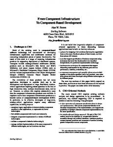
Component-based software engineering (CBSE) [17, 18] is widespread in enterprise computing. A component is an atomic unit of software encapsulating some useful functionality, interacting with the outside world through well-defined interfaces often specified in an interface definition language. Components are composed into applications, which are executed in a runtime framework. CBSE enables software reuse, empowers application developers to switch between subsystem implementations for which multiple components exist, and can dramatically reduce application development time. Examples of commercial CBSE approaches include COM, DCOM, JavaBeans, Rails, and CORBA. Alas, they are not suitable for scientific applications for two reasons: unreasonably high performance cost, especially in massively parallel applications, and inability to describe scientific data adequately (e.g., they do not support complex numbers). The Common Component Architecture (CCA) [19, 20] is a CBSE approach targeting high-performance scientific computing. CCA’s approach is based on explicit descriptions of software dependencies (i.e., caller/callee relationships). CCA component interfaces are known as ports: provides ports are the interfaces implemented, or provided, by a component, while uses ports are external interfaces whose methods are called, or used, by a component. Component interactions follow a peer component model through a connection between a uses ports and a provides port of the same type to establish a caller/callee relationship (Figure 1 (a)). The CCA specification also defines some special ports (e.g., GoPort, essentially a “start button” for a CCA application). CCA interfaces as well as port and component definitions are described in a SIDL (scientific interface definition language) file, which is subsequently processed by a language interoperability tool such as Babel [21] to create the necessary interlanguage glue code. CCA meets performance criteria associated with high-performance computing, and typical latency times for intercomponent calls between components executing on the same parallel machine are on the order of a virtual function call between same-language components; times for interlanguage component interactions are slightly more, but within 1–2 orders of magnitude of typical MPI latency times. The port connection and mediation of calls is handled by a CCA-compliant framework. Each component implements a SetServices() method where the component’s uses and provides ports are registered with the framework. At runtime, uses ports are connected to provides ports, and a component can access the methods of a port through a getPort() method. A typical port connection diagram for a simple application (which will be discussed in greater detail in Section 6) is shown in Figure 1 (b). CCA technology has been applied successfully in many application areas including combustion, computational chemistry, and Earth sciences. CCA’s language interoperability approach has been leveraged to create multilingual bindings for the Model Coupling Toolkit (MCT) [22], the coupling middleware used by


61

Fig. 1. Sample CCA component wiring diagrams: (a) generic port connection for two components; (b) a simple application composed from multiple components.

the Community Climate System Model (CCSM), and a Python implementation of the CCSM coupler. The work reported here will eventually be part of the CCA Toolkit.

4

PCI Component Toolkit

Our PCI specification is designed to address the majority of the requirements stated in Section 2.3. Emphasis is on the parallel data processing part of the PCP, with a middleware layer immediately above MPI that models can invoke to perform parallel coupling operations. A highly modular approach that separates concerns at this low level maximizes flexibility, and this bottom-up design allows support for serial and parallel compositions and multiple executables. We have defined a standard API for distributed data description and constituent processor layout. These standards form a foundation for an API for parallel data transfer and transformation. Below we outline the PCI API and the component and port definitions for PCI-Tk. 4.1

Data Model for Coupling

ˆ i (Γi ) In our specification, the objects for data description are the SpatialGrid (D ˆ ˆ ˆ and Di (∂Γi )), the FieldData (the input and output vectors Vi and Wi ) and the GlobalIndMap (the domain decomposition Pi ). This approach assumes a 1-1 mapping between the elements of the spatial discretization and the physical locations in the field data definition. The domain decomposition applies equally to both. For example, a constituent Ci spread across a cohort of Ki processors, each ˆ ki (∂Γi ), and processor (say, the kth) will have its own SpatialGrid to describe D ˆ k, ˆ k and W FieldData instantiations to describe its local inputs and outputs V i i respectively. In the interest of generality and minimal burden to PCI implementers, we have adopted explicit virtual linearization [11,2,23,24,25,26] as our

62


index and mesh description standard. Virtual linearization supports decomposition description of multidimensional index spaces and meshes, both structured and unstructured. We have adopted an explicit, segmented domain decomposition [2, 11] of the linearized index space. Data transfer within PCI requires a description of the constituents’ cohorts and communications schedules for interconstituent parallel data transfers and intracohort parallel data redistributions. Mapping of constituent processor pools is described by the CohortRegistry interface, which provides MPI processor ID ranks for a constituent’s processors within its own MPI communicator and a union communicator of all model cohorts. The CohortRegistry provides lookup services necessary for interconstituent data transfers. Our PCI data model provides two descriptors for the transfer operation Hji : The TransferSched API is an interface that encapsulates interconstituent parallel data transfer scheduling; that is, it contains all of the information necessary to execute all of the MPI point-to-point communication calls needed to implement the transfer. The data transformation part of the PCI requires data models for linear transformations and for time integration. The LinearTransform encapsulates the whole transformation from storage of transformation coefficients to communications scheduling required to execute the parallel transformation. The TimeIntRegister describes time integration and averaging registers required for loose coupling in which state averages and flux integrals are exchanged periodically for incremental application. In the SIDL PCI API, all of the elements of the data model are defined as interfaces; their implementation as classes or otherwise is at the discretion of the PCI developer. 4.2

PCI-Tk Components

Data Description The Fabricator Component. The Fabricator creates objects used in the interfaces for all the coupling components, along with their associated service methods. It also handles overall MPI communicator management This component has a single provides port, Factory, on which all of the create/destroy, query, and manipulation methods for the coupling data objects reside. Data Transfer. Data under transfer by our PCI interfaces is described by our FieldData specification. The Transporter Component. The Transporter performs one-way parallel data transfers such as the data routing between source and destination constituents, with communications scheduling described by our TransferSched interface. It has one provides port, Transfer, on which methods for both blocking (PCI Send(), PCI Recv()) and nonblocking (PCI ISend(), PCI IRecv()) parallel data transfers are implemented, making it capable of supporting both serial and parallel compositions.


63

The Transposer Component. The Transposer performs two-way parallel data transfers such as data redistribution within a cohort, or two-way data traffic between constituents, with communications scheduling defined by the TransposeSched interface. It has one provides port, Transpose, that implements a data transpose function PCI Transpose(). Data Transformation. The data transformation components in PCI-Tk act on FieldData inputs and, unless otherwise noted, produce outputs described by the FieldData specification. The LinearTransformer Component. The LinearTransformer performs parallel linear transformations using user-defined, precomputed transform coefficients. It has a single provides port, LinearXForm, that implements the transformation method PCI ApplyLinearTransform(). The TimeIntegrator Component. The TimeIntegrator performs temporal integration and averaging of FieldData for a given constituent, storing the ongoing result in a form described by the TimeIntRegister specification. It has a single provides port, TimeInt, that implements methods for time averaging and integration, named PCI TimeIntegral() and PCI TimeAverage(), respectively. Users can retrieve time integrals in FieldData form from a query method associated with the TimeIntRegister interface. The SpatialIntegrator Component. The SpatialIntegrator performs spatial integrals of FieldData on its resident SpatialGrid. It has a single provides port, SpatialInt, that offers methods PCI SpatialIntegral() and PCI SpatialAverage() that perform multifield spatial integrals and averages, respectively. This port also has methods for performing simultaneously paired multifield spatial integrals and averages; here pairing means that calculations for two different sets of FieldData on their respective resident SpatialGrid objects are computed. This functionality enables efficient, scalable diagnosis of conservation of fluxes under transformation from source to target grids. The Merger Component. The Merger merges data from multiple sources that have been transformed onto a common, shared SpatialGrid. It has a single provides port, Merge, on which merging methods reside, including PCI Merge2(), PCI Merge3(), and PCI Merge4() for merging of data from two, three, and four sources, respectively. An additional method PCI MergeIn() supports higherorder and other user-defined merging operations.

5

Reference Implementation

We are using MCT to build a reference implementation of our PCI specification. MCT provides a data model and library support for parallel coupling. Like the specification, MCT uses virtual linearization to describe multidimensional index

64

J.W. Larson and B. Norris Table 1. Correspondence between PCI Data Interfaces and MCT Classes

Functionality ˆ i Γi , D ˆ i (∂Γi ) Mesh Description D ˆ i, V ˆ i, W î Field Data U Domain Decomposition Pi Constituent PE Layouts One-Way Parallel Data Transfer Scheduling Hij Two-Way Parallel Data Transpose Scheduling Hij Linear Transformation Gij Time Integration Registers

PCI Interface SpatialGrid FieldData GlobalIndMap CohortRegistry TransferSched TransposeSched LinearTransform

MCT Class GeneralGrid AttrVect GlobalSegMap MCTWorld Router Rearranger SparseMatrix SparseMatrixPlus TimeIntRegister Accumulator

Table 2. Correspondence between PCI Ports and MCT Methods Component / Port Fabricator / Factory

MCT Method Create, destroy, query, and manipulation methods for GeneralGrid, AttrVect, GlobalSegMap, MCTWorld, Router, Rearranger, SparseMatrix, SparseMatrixPlus, and Accumulator Transporter / Transfer Transfer Routines MCT Send(), MCT Recv(), MCT ISend(), MCT IRecv(), Transposer / Transpose Rearrange() LinearTransform / LinearXForm SparseMatrix-AttrVect Multiply sMatAvMult() SpatialIntegrator / Spatial Integral SpatialIntegral() and SpatialAverage() TimeIntegrator / TimeIntegral accumulate() Merger / Merge Merge()

spaces and grids. MCT’s Fortran API is described in SIDL, and Babel has been used to generate multilingual bindings [22], with Python and C++ bindings and example codes available from the MCT Web site. The data model from our PCI specification maps readily onto MCT’s classes (see Table 1). The port methods are implemented in some cases through direct use (via glue code) of MCT library routines, and at worst via lightweight wrappers that perform minimal work to convert port method arguments into a form usable by MCT. Table 2 shows in broad terms how the port methods are implemented.

6

Deployment Examples

We present three examples from climate modeling in which PCI-Tk components could be used to implement parallel couplings. the field of coupled climate modeling. In each example, the system contains components for physical subsystems and a coupler. The coupler handles the data transformation, and the models interact via the coupler purely through data transfers—a hub-and-spokes architecture [15].


65

The MCT toy climate coupling example comprises atmosphere and ocean components that interact via a coupler that performs intergrid interpolation, and computes application-specific variable transformations such as computation of interfacial radiative fluxes. It is a single executable application; the atmosphere, ocean, and coupler are procedures invoked by the MAIN driver application. It is a parallel composition; parallel data transfers between the cohorts are required. A CCA wiring diagram of this application using PCI-Tk components is shown in Figure 1 (b). The driver component with the Go port signifies the single executable, and this component has uses ports labeled Atm, Ocn, and Cpl implemented as provides ports on the atmosphere, ocean, and coupler components, respectively. The PCI-Tk data model elements used in the coupling are created and managed by the Fabricator, via method calls on its Factory port. The parallel data transfer traffic between the physical components and the coupler are implemented by the Transporter component via method calls on its Transfer port. A LinearTransform component is present to implement interpolation between the atmosphere and ocean grids; the coupler performs this task via method calls on its LinearXform port. The Parallel Climate Model (PCM) example [6] shown in Figure 2 (a) is a single executable and a serial composition. A driver coordinates execution of the individual model components. Since the models run as a serial composition, coupling data can be passed across interfaces, and transposes performed as needed; thus there is a Transpose component rather than a Transfer component. The coupler in this example performs the full set of transformations found in PCM: intergrid interpolation with the LinearTransform; diagnosis of flux conservation under interpolation with the SpatialIntegrator; time integration of flux and

Fig. 2. CCA wiring diagrams for a two coupled climate model architectures: (a) PCM, with serial composition and single executable; (b) CCSM, with parallel composition and multiple executables

66


averaging of state data using the TimeIntegrator; and merging of data from multiple sources with the Merger. The TimeIntegrator is invoked by both the ocean and coupler components because of the loose coupling between the ocean and the rest of PCM; the atmosphere, sea-ice, and land-surface models interact with the couple hourly, but the ocean interacts with the coupler once per model day. The coupler integrates the hourly data from the atmosphere, land, and sea-ice that will be passed to the ocean. The ocean integrates its data from each timestep over the course of the model day for delivery to the coupler. The CCSM example is a parallel composition. Its coupling strategy is similar to that in PCM in terms of the parallel data transformations and implementation of loose coupling to the ocean. CCSM uses a peer communciation model, however, with each of the physical components communicating in parallel with the coupler. These differences are shown in Figure 2 (b). The atmosphere, ocean, sea-ice, landsurface, and coupler are separate executables and have Go ports on them; and the parallel data transfers are implemented by the Transfer component rather than the Transpose component.

7

Conclusions

Coupling and the PCP are problems of central importance as computational science enters the age of multiphysics and multiscale models. We have described the theoretical underpinnings of the PCP and derived a core set of PCI requirements. From these requirements, we have formulated a PCI component interface specification that is compliant with the CCA, a component approach suitable for high-performance scientific computing—a parallel coupling infrastructure toolkit (PCI-Tk). We have begun a reference implementation based on the Model Coupling Toolkit MCT. Use-case scenarios indicate that this approach is highly promising for climate modeling applications, and we believe the reference implmentation will perform approximately as well as MCT does: the component overhead introduced by CCA has been found to be acceptably low in other application studies [19]; and our own performance studies on our Babel-generated C++ and Python bindings for MCT show minimial performance impact (at most a fraction of a percent versus the native Fortran implementation [22]). Future work includes completing the reference implementation and a thorough performance study; prototyping of applications using the MCT-based PCI-Tk; modifying the specification if necessary; and exploring alternative PCI component implementations (e.g., using mesh and field data management tools from the DOE-supported Interoperable Technologies for Advanced Petascale Simulations (ITAPS) center [27]. Acknowledgements. This work is primarily a product of the Center for Technology for Advanced Scientific Component Software (TASCS), which is supported by the US Department of Energy (DOE) Office of Advanced Scientific Computing Research through the Scientific Discovery through Advanced Computing Program, . Argonne National Laboratory is managed for the DOE by UChicago Argonne LLC under supported by the DOE under contract DE-AC02-06CH11357.


67

The ANU Supercomputer Facility is funded in part by the Australian Department of Education, Science, and Training through the Australian Partnership for Advanced Computing (APAC).

References 1. Manabe, S., Bryan, K.: Climate calculations with a combined ocean-atmosphere model. Journal of the Atmospheric Sciences 26(4), 786–789 (1969) 2. Larson, J., Jacob, R., Ong, E.: The Model Coupling Toolkit: A new Fortran90 toolkit for building multi-physics parallel coupled models. Int. J. High Perf. Comp. App. 19(3), 277–292 (2005) 3. Larson, J.W.: Some organising principles for coupling in multiphysics and multiscale models. Preprint ANL/MCS-P1414-0207, Mathematics and Computer Science Division, Argonne National Laboratory (2006) 4. Bryan, F.O., Kauffman, B.G., Large, W.G., Gent, P.R.: The NCAR CSM flux coupler. NCAR Tech. Note 424, NCAR, Boulder, CO (1996) 5. Jacob, R., Schafer, C., Foster, I., Tobis, M., Anderson, J.: Computational design and performance of the Fast Ocean Atmosphere Model. In: Alexandrov, V.N., Dongarra, J.J., Juliano, B.A., Renner, R.S., Tan, C.J.K. (eds.) ICCS 2001. LNCS, vol. 2073, pp. 175–184. Springer, Heidelberg (2001) 6. Bettge, T., Craig, A., James, R., Wayland, V., Strand, G.: The DOE Parallel Climate Model (PCM): The Computational Highway and Backroads. In: Alexandrov, V.N., Dongarra, J.J., Juliano, B.A., Renner, R.S., Tan, C.J.K. (eds.) ICCS 2001. LNCS, vol. 2073, pp. 148–156. Springer, Heidelberg (2001) 7. Drummond, L.A., Demmel, J., Mechose, C.R., Robinson, H., Sklower, K., Spahr, J.A.: A data broker for distirbuted computing environments. In: Alexandrov, V.N., Dongarra, J.J., Juliano, B.A., Renner, R.S., Tan, C.J.K. (eds.) ICCS 2001. LNCS, vol. 2073, pp. 31–40. Springer, Heidelberg (2001) 8. Valcke, S., Redler, R., Vogelsang, R., Declat, D., Ritzdorf, H., Schoenemeyer, T.: OASIS4 user’s guide. PRISM Report Series 3, CERFACS, Toulouse, France (2004) 9. Hill, C., DeLuca, C., Balaji, V., Suarez, M., da Silva, A.: The ESMF Joint Specification Team: The architecture of the earth system modeling framework. Computing in Science and Engineering 6, 18–28 (2004) 10. Toth, G., Sokolov, I.V., Gombosi, T.I., Chesney, D.R., Clauer, C.R., Zeeuw, D.D., Hansen, K.C., Kane, K.J., Manchester, W.B., Oehmke, R.C., Powell, K.G., Ridley, A.J., Roussev, I.I., Stout, Q.F., Volberg, O., Wolf, R.A., Sazykin, S., Chan, A., Yu, B., Kota, J.: Space weather modeling framework: A new tool for the space science community. Journal of Geophysical Research 110, A12226 (2005) 11. Bertrand, F., Bramley, R., Bernholdt, D.E., Kohl, J.A., Sussman, A., Larson, J.W., Damevski, K.B.: Data redistribution and remote method invocation for coupled components. Journal of Parallel and Distributed Computing 66(7), 931–946 (2006) 12. Joppich, W., Kurschner, M.: MpCCI - a tool for the simulation of coupled applications. Concurrency and Computation: Practice and Experience 18(2), 183–192 (2006) 13. Jacob, R., Larson, J., Ong, E.: M x N communication and parallel interpolation in ccsm3 using the Model Coupling Tookit. Int. J. High Perf. Comp. App. 19(3), 293–308 (2005) 14. The MCT Development Team: Model Coupling Toolkit (MCT) web site (2007), http://www.mcs.anl.gov/mct/

68


15. Craig, A.P., Kaufmann, B., Jacob, R., Bettge, T., Larson, J., Ong, E., Ding, C., He, H.: cpl6: The new extensible high-performance parallel coupler for the community climate system model. Int. J. High Perf. Comp. App. 19(3), 309–327 (2005) 16. Foster, I.: Designing and Building Parallel Programs: Concepts and Tools for Parallel Software Engineering. Addison Wesley, Reading, Massachusetts (1995) 17. Szyperski, C.: Component Software: Beyond Object-Oriented Programming. ACM Press, New York (1999) 18. Heineman, G.T., Council, W.T.: Component Based Software Engineering: Putting the Pieces Together. Addison-Wesley, New York (1999) 19. Bernholdt, D.E., Allan, B.A., Armstrong, R., Bertrand, F., Chiu, K., Dahlgren, T.L., Damevski, K., Elwasif, W.R., Epperly, T.G.W., Govindaraju, M., Katz, D.S., Kohl, J.A., Krishnan, M., Kumfert, G., Larson, J.W., Lefantzi, S., Lewis, M.J., Malony, A.D., Mclnnes, L.C., Nieplocha, J., Norris, B., Parker, S.G., Ray, J., Shende, S., Windus, T.L., Zhou, S.: A component architecture for high-performance scientific computing. Int. J. High Perf. Comp. App. 20(2), 163–202 (2006) 20. CCA Forum: CCA Forum web site (2007), http://cca-forum.org/ 21. Dahlgren, T., Epperly, T., Kumfert, G.: Babel User’s Guide. CASC, Lawrence Livermore National Laboratory. version 0.9.0 edn. (January 2004) 22. Ong, E.T., Larson, J.W., Norris, B., Jacob, R.L., Tobis, M., Steder, M.: Multilingual interfaces for parallel coupling in multiphysics and multiscale systems. In: Shi, Y. (ed.) ICCS 2007. LNCS, vol. 4487, pp. 924–931. Springer, Heidelberg (2007) 23. Lee, J.-Y., Sussman, A.: High performance communication between parallel programs (Appears with the Proceedings of IPDPS 2005). In: Proceedings of 2005 Joint Workshop on High-Performance Grid Computing and High-Level Parallel Programming Models (HIPS-HPGC 2005), Apr 2005, IEEE Computer Society Press, Los Alamitos (2005) 24. Sussman, A.: Building complex coupled physical simulations on the grid with InterComm. Engineering with Computers 22(3–4), 311–323 (2006) 25. Jones, P.W.: A user’s guide for SCRIP: A spherical coordinate remapping and interpolation package. Technical report, Los Alamos National Laboratory, Los Alamos, NM (1998) 26. Jones, P.W.: First and second-order conservative remapping schemes for grids in spherical coordinates. Mon. Wea. Rev. 127, 2204–2210 (1999) 27. Interoperable Technologies for Advanced Petascale Simulation Team: ITAPS web site (2007), http://www.scidac.gov/math/ITAPS.html