Composite Proximal Bundle Method - Optimization Online

Composite Proximal Bundle Method Claudia Sagastiz´abal∗

Abstract We consider minimization of nonsmooth functions which can be represented as the composition of a positively homogeneous convex function and a smooth mapping. This is a sufficiently rich class that includes max-functions, largest eigenvalue functions, and norm-1 regularized functions. The bundle method uses an oracle that is able to compute separately the function and subgradient information for the convex function, and the function and derivatives for the smooth mapping. With this information, it is possible to solve approximately certain proximal linearized subproblems in which the smooth mapping is replaced by its Taylor-series linearization around the current serious step. Our numerical results show the good performance of the Composite Bundle method for a large class of problems.

1

Introduction and motivation

For some years already, nonsmooth optimization research has focused on exploiting structure in the objective function as a way to speed up numerical methods. Indeed, for convex optimization, complexity results establish that oracle based methods have a linear rate of convergence; [NY83]. The U-Lagrangian theory [LS97], [LOS00], and the VU-space decomposition [MS00], can be seen as tools to “extract” smooth structure from general convex functions. The approach was extended to a class of nonconvex functions in [MS04]. Similar ideas for more general nonconvex functions, having a smooth representative on a certain manifold corresponding to the U-subspace, are explored in [Lew02], [Har03]. Another line of work concentrates efforts on identifying classes of functions structured enough to have some type of second-order developments, such as the primal-dual gradient structured functions from [MS00], [MS03], or the composite functions in [Sha03]. Composite functions, that were first considered in [Fle87, Ch. 14], and studied in [BF95], [LW02], have been more recently revisited in [Nes07] and [LW08], in the convex and nonconvex settings, respectively. Most of the work above is conceptual, in the sense that if some algorithmic framework is considered, often it is not implementable. Among the exceptions, we find the convex optimization algorithms in [Ous00], [MS05], [Nes07], and the V-space identification method in [DSS09]. In this paper, we develop an implementable bundle method that exploits structure for certain nonconvex composite optimization problems. More precisely, given a smooth mapping c : 0 such that (13) holds for any µ` > µnoBT . (ii) There cannot be infinitely many consecutive backtracking steps. ˆ ˆ = k(`), ˆ x ˆ and M ˆ = Mˆ denote, respectively, Proof: For convenience, let k ˆ = xk (= xk(`) for all ` ≥ `), k the k-iteration index, prox-center and matrix corresponding to the last serious step. Since c is a C 2 -mapping, a mean-value theorem applies to each component cj , j = 1, . . . , m:

cj (ˆ x + d` ) − cj (ˆ x) − ∇cj (ˆ x)> d` =

1 2 ∇ cj (ξj )(d` , d` ) 2

for some ξj ∈ [ˆ x, x ˆ + d` ] .

Recall that | · | is the Euclidean matrix norm. By assumption, {ˆ x + d` } is bounded so |Γ` | ≤ L for all ` ` and some constant L. Similarly, boundedness of {d } implies that |∇2 cj (ξj )| ≤ D for all j = 1, . . . , m, for some constant D. By Cauchy-Schwarz inequality, √ m LD|d` |2 . Γ` > [c(ˆ x + d` ) − c(ˆ x) − Dkˆ d` ] ≤ 2 Using the rightmost inequality in (17)(b), we obtain δ` ≥

1 `2 1 ˆ ) + µ` )|d` |2 . |d |k,` (λmin (M ˆ ≥ 2 2

In the notation used in this proof, c(xk + d` ) = c(ˆ x + d` ) and ck (d` ) = c(ˆ x) + Dkˆ d` . Suppose that (13) is not satisfied and multiply by −1 the corresponding inequality: m2 δ` < −Γ` > [ck (d` ) − c(xk + d` )] = Γ` > [c(ˆ x + d` ) − c(ˆ x) − Dkˆ d` ] . Using the bounds above we see that √ 1 m ˆ ) + µ` )|d` |2 ≤ m2 δ` < Γ` > [c(ˆ m2 (λmin (M x + d` ) − c(ˆ x) − Dkˆ d` ] ≤ LD|d` |2 . 2 2 √ ˆ ). Item (i) follows, by taking Therefore, nonsatisfaction of (13) implies µ` < mLD/m2 − λmin (M √ µnoBT ≥ mLD/m2 − λmin (Mk ). The claim in item (ii) is shown by contradiction, assuming that (13) does not hold, with ` → ∞ due to backtracking. An infinite backtracking loop drives µ` to infinity, as well as the minimum eigenvalue ˆ + µ` I. Since there are only backtracking steps, the bundle does of the matrix Mkˆ` , because Mkˆ` = M ˇ ` (cˆ (·)) is a fixed function, say ϕ. Hence, by [HUL93, Prop. not change, and the composite model h k XV.4.1.5], the minimand in (9) converges to ϕ(d) for all d ∈ G k (iii) If, in addition, the sequence {xk } is bounded, then it has at least one accumulation point that is critical for (1). (iv) If, instead of (18), the stronger condition the sequence {µ`k + λmax (Mk )} is bounded above,

(18’)

then all accumulation points are critical for (1). Proof: By (13), since Γ`k ∈ ∂h(c(xk + d`k )), we have that h(c(xk ) + Dk d`k ) ≥ h(c(xk + d`k )) − m2 δ`k = (h ◦ c)(xk+1 ) − m2 δ`k .

(19)

Together with satisfaction of (12), this means that (h ◦ c)(xk+1 ) ≤ (h ◦ c)(xk ) − (m1 − m2 )δ`k . The telescopic sum yields that either (h ◦ c)(xk ) & −∞ or 0 ≤ δ`k → 0, because m1 − m2 > 0. The first assertion in item (ii) follows from (11). The rightmost inequality in (17)(a), together with our assumption (18) gives the second result. ˆ `k kk,` → 0 and extract a further subseTo show item (iii), consider a k-subsequence such that kDk> G k quence of serious steps with accumulation point xacc . By boundedness of {xk } and local Lipschitzianity ˆ ` } with accumulation point G ˆ acc . Passing to the limit in (16) of h, there is an associated subsequence {G acc acc ˆ ∈ ∂h(C ) for C acc = c(xacc ). By smoothness and using that eˆ`k → 0, we obtain in the limit that G > ˆ acc ∈ ∂(h ◦ c)(xacc ). The result follows from item (ii). of c, Dk → Dacc = Dc(xacc ), and by (2), Dacc G Item (iv) is similar to item (iii), noticing that if L > 0 denotes an upper bound for {µ`k + λmax (Mk )}, ˆ `k | → 0 as k → ∞ (for the whole then the relation 2(µ` +λ1max (Mk ) ≥ 1/2L in (17)(b) gives that |Dk> G k

u t

sequence). The remaining case refers to an infinite null-step loop and makes use of the aggregate linearization ˇ agg (ck (d)) = h ˇ ` (ck (d` )) + G ˆ ` > Dk (d − d` ) , h ` the associated strongly convex function ˇ agg (ck (d)) + H` (d) = h `

1 2 |d|k,` , 2

(20)

and the result [HUL93, Lem. XV.4.3.3]: 1 |d − d`−1 |2k,`−1 . (21) 2 Finally, and similar to [CL93, Sec. 4], note that Step 4 in Algorithm 1 updates the bundle of information in a way ensuring that not only H`−1 (d) = H`−1 (d`−1 ) +

if iteration ` − 1 was declared a null step, then

ˇ agg (ck (d)) ≤ h ˇ ` (ck (d)) , h `−1

(22)

if iteration ` − 1 was declared a null step, then for all d ∈ < .

ˇ ` (ck (d)) ≥ G`−1 > ck (d) h

(23)

but also n

10

ˆ Algorithm 1 makes a Lemma 2 (Finitely many serious steps) Suppose that, after some iteration `, last serious step x ˆ=x ˆk(`) and thereafter generates an infinite number of null steps, possibly nonconsecutive, due to intermediate backtracking steps. The following holds: (i) The sequence {d` }`>`ˆ is bounded and there is an iteration `0 > `ˆ such that only null steps are done for all ` ≥ `0 . (ii) If m1 < 1, then δ` → 0 and eˆ` → 0. ˆ =M ˆ. (iii) If, in addition, for the (fixed) matrix M k(`) the series

X µ`−1 + λmin (M ˆ) is divergent, ˆ (µ` + λmax (M ))2 `≥`0

(24)

ˆ ` | = 0, x then lim inf |Dc(ˆ x)> G ˆ + d` → x ˆ for some `-subsequence, and x ˆ is critical for (1). ˆ ˆ = k(`), ˆ x ˆ and M ˆ = Mˆ denote, respectively, Proof: For convenience, let k ˆ = xk (= xk(`) for all ` ≥ `), k the k-iteration index, prox-center and matrix corresponding to the last serious step. ˆ +µ` I and {µ` } is nondecreasing at null and backtracking Consider ` > `ˆ and recall that, since Mk` = M steps, 1 1 2 |d|ˆ ≤ |d|2k,` ˆ . 2 k,`−1 2 The sum of this inequality and (22), together with (20) written with ` replaced ` − 1, results in the relation ˇ ` (cˆ (d)) + 1 |d|2ˆ . H`−1 (d) ≤ h k 2 k,` ` ` ` ˇ ` (cˆ (d` )) = h ˇ agg (cˆ (d` )). In particular, for d = d , we obtain that H`−1 (d ) ≤ H` (d ) from (20), because h ` k k ` Together with (21), written at d = d , we see that

H`−1 (d`−1 ) ≤ H`−1 (d`−1 ) +

1 ` |d − d`−1 |2k,`−1 = H`−1 (d` ) ≤ H` (d` ) . ˆ 2

(25)

ˇ agg and H` , the optimal value in (9) equals H` (d` ). Hence, (25) implies that the By the definitions of h ` ˇ ` (ck (0)) = h ˇ ` (c(ˆ sequence of optimal values in (9) is strictly increasing, with H` (d` ) ≤ h x)). Since, by ˇ ` ≤ h, then (15), h H` (d` ) ≤ (h ◦ c)(ˆ x) . (26) → 0 as ` → ∞, by (25). But µ` ≥ µ`ˆ So {H` (d` )} ↑ H∞ for some H∞ ≤ (h ◦ c)(ˆ x), with |d` − d`−1 |2k,`−1 ˆ (at null and backtracking steps prox-parameters are nondecreasing), so the left relation in (8) implies that d` − d`−1 → 0 . (27) agg agg ˇ ˇ Using (20) with d = 0, we see that H` (0) = h` (ckˆ (0)). Together with the definition of h` , the left inequality in the second line in (10), and the definition of ck (d` ), this implies that that H` (0) = ˇ ` (cˆ (d` )) − G ˆ ` > D ˆ d` = G ˆ ` > c(ˆ ˆ ` ∈ conv{Gi : i ∈ B` }, using (5) and (3) we obtain that h x). Since G k k H` (0) ≤ (h ◦ c)(ˆ x). Therefore, writing (21) with ` − 1 replaced by ` at d = 0 yields the relations ˆ 1 `2 ` `+1 |d |k,` x) − H`+1 ), ˆ (d ˆ = H` (0) − H` (d ) ≤ (h ◦ c)(ˆ 2

ˆ Using once more the left relation in because the sequence {H` (d` )} is increasing, by (25), since ` > `. (8) we conclude that the sequence {d` } is bounded, and item (i) follows from Proposition 1(i). To show item (ii), consider iteration indices ` − 1, ` ≥ `0 , giving two consecutive null steps, and set C ` = c(ˆ x) + Dc(ˆ x)d` and C `−1 = c(ˆ x) + Dc(ˆ x)d`−1 . Since δ` ≥ 0, we substract the inequality δ` ≤ ` ˇ (h ◦ c)(ˆ x) − h` (C ), obtained from (11), from nonsatisfaction of (12), both with xk = x ˆ, to see that ˇ ` (C ` ) . 0 ≤ (1 − m1 )δ` ≤ h(C ` ) − h By (3), h(C `−1 ) = G`−1 > C `−1 ,

11

(28)

and by (23), ˇ ` (cˆ (d` )) = h ˇ ` (C ` ) ≥ G`−1 > C ` . h k Since {d` } is bounded, any Lipschitz constant L for h gives an upper bound for {|G` |}; as a result, ˇ ` (C ` ) h(C ` ) − h

=

ˇ ` (C ` ) h(C ` ) − h(C `−1 ) + h(C `−1 ) − h

≤

L|C ` − C `−1 | + G`−1 > (C `−1 − C ` )

≤

2L|Dc(ˆ x)||d` − d`−1 | .

(29)

From (28) and (27) it follows that δ` → 0, and by the right hand side expression in (11), eˆ` → 0, as stated. ˇ agg and H` Finally, to see item (iii), the left hand side expression in (11) of δ` and the definitions of h ` ` give the identity δ` = (h ◦ c)(ˆ x) − H` (d ). Therefore, by the right inequality in (25), (22) with d = d` , and the left relation in (8), δ`−1

≥ ≥

1 ` |d − d`−1 |2k,`−1 ˆ 2 ˆ ) + µ`−1 ` λmin (M δ` + |d − d`−1 |2 . 2 δ` +

From (29) and (28), we obtain that δ` ≤ δ`−1 − δ` ≥

2L|Dc(ˆ x)| ` |d 1−m1

− d`−1 |, so

ˆ ) + µ`−1  1 − m1 2 2 λmin (M δ` . 2 2L|Dc(ˆ x)|

  ˆ Letting K := (1 − m1 )2 / 8|Dc(ˆ x)|2 L2 , and summing over ` > `, K

X ˆ ) + µ`−1 )δ`2 ≤ δ ˆ < +∞ . (λmin (M ` `>`ˆ

Furthermore, using (17)(a), the series X µ`−1 + λmin (M ˆ) ˆ ` |4 |Dc(ˆ x)> G ˆ (µ + λ ( M ))2 max ` ˆ `>`

ˆ ` |4 = 0. Consider indices ` in converges too. With our assumption (24), this implies that lim inf |Dc(ˆ x)> G ` ˆ ` |2 = a corresponding convergent subsequence of {d }. Since from the expression for d` in (10), |Dc(ˆ x)> G ` ` 2 2 ` 2 ` ˆ |Mk d | ≥ (λmin (M )+µ`ˆ) |d | , we see that the subsequence fo {d } converges to zero and, hence, x ˆ+d` → x ˆ on this subsequence. Finally, by boundedness of {C ` = c(ˆ x) + Dc(ˆ x)d` }, all outer subgradients are ˆ acc = 0. ˆ ` } has some accumulation point G ˆ acc such that Dc(ˆ bounded and, hence, the subsequence {G x)> G acc ˆ The result follows from passing to the limit in (16) to give G ∈ ∂h(c(ˆ x)), and using the chain rule (2). u t Remark 2 (The trivial composite case, suite and end.) In the setting of Remark 1, when h is not positively homogeneous but merely convex, and c is the identity, the cutting-planes model has the form (6) and (23) states that if iteration ` − 1 was declared a null step, then

ˇ ` (ck (d)) ≥ h(xk ) − ∆k`−1 + G`−1 > ck (d) , h

which is consistent with the fact that h(xk ) = ∆k`−1 when h is positively homogenous, by (5) and (3). In fact, when Mk ≡ 0 for all k, as considered in the trivial structure, Lemmas 1 and 2 boil down to [HUL93, pp.309 and 311, vol.II, Thms.XV.3.2.2 and XV.3.2.4]. Putting together Proposition 1 and Lemmas 1 and 2, we can show convergence for objective functions that are inf-compact, i.e., functions having some level set that is nonempty and compact (sometimes also referred to as level-bounded functions). In this case, by lower semicontinuity, h ◦ c always attains its minimum and the sequence of serious steps is bounded.

12

Theorem 1 (Synthesis) Consider solving problem (1) with Algorithm 1 and suppose that in (1) the objective function h ◦ c is inf-compact. If 0 < m2 < m1 < 1, tolstop = 0, with both (18) and (24) being satisfied, the following holds. (i) Either the sequence of serious steps is infinite and bounded, and at least one of its accumulation points is critical for (1). (ii) Or the last serious step x ˆ is critical for (1), with {ˆ x + d` } → x ˆ for some `-subsequence. If, instead of (18), the stronger condition (18’) holds, item (i) can be replaced by (i’) Either the sequence of serious steps is infinite and bounded, and all its accumulation points are critical for (1). u t Our conditions (18) and (24), on the variable prox-metric, are fairly general and not difficult to enforce. For (18) to hold, it is enough to take matrices Mk` that are uniformly bounded from above at serious steps (when ` = `k ). As for null steps, choosing µ`+1 ∈ [µ` , µmax ] for some finite bound ˆ ), rule (14) ensures satisfaction of (24). Depending on the particular problem, the µmax > −λmin (M more general condition (24) may help in preventing bad choices (too small) for the bound µmax . We finish our analysis by supposing the stopping tolerance is positive. In this case, if (18’) and (24) ˆ ` go to 0, hold, by Lemmas 1 and 2, the nominal decrease goes to 0. Then, by (11), both eˆ` and G and eventually the stopping test will be triggered. For such an iteration index, say `best, (16) gives the following approximate optimality condition for the last serious step xbest = xk(`best) :   ˆ `best > c(x) − c(xbest ) − eˆ`best ∀x ∈ Dc(xbest )(x − xbest ) + o(|x − xbest |) − eˆ`best ≥ (h ◦ c)(xbest ) − G ≥

6

(h ◦ c)(xbest ) − tolstop |x − xbest | − tolstop + o(|x − xbest |) .

Numerical experience

In order to assess from a practical point of view the Composite Bundle method, we coded Algorithm 1 in matlab and ran it on several collections of functions described in Sec. 2, using a computer with one 3GHz processor and 1.49GB RAM.

6.1

Solvers in the benchmark

We compared the performance of the Composite Bundle method with the Matlab HANSO package, implementing a “Hybrid Algorithm for NSO”, and downloadable from http://cs.nyu.edu/overton/ software/index.html. As explained in [LO08], for nonsmooth optimization problems, BFGS may fail theoretically. However, the HANSO package can provide good benchmarks for the purpose of comparison, helping to shed some light on important NSO issues, as shown in our results below. The package is organized in two phases: – A first phase runs a BFGS method for smooth unconstrained optimization, with a linesearch capable of handling kinks explained in [LO08], and with multiple starting points. If the termination test is not satisfied at the best point found by BFGS, HANSO continues to the next phase. – The second phase executes up to three runs of the Gradient Sampling method in [BLO02], starting from the lowest point found by BFGS, and with decreasing sampling radii. As initial information, the Gradient Sampling uses BFGS final bundle, corresponding to the last min[100, 2n, n + 10] generated points and their (bb) information. For locally Lipschitz functions, the method converges to Clarke critical points in a probabilistic sense; [BLO02]. We also created another hybrid algorithm, the Hybrid Composite Bundle, that after the BFGS phase switches to the Composite Bundle method, starting like Hanso from BFGS’s final bundle. Therefore, the benchmark considers the four solvers below: – CBun, the Composite Bundle method, – BFGS, the first phase in the HANSO package, – Hanso, the hybrid variant combining BFGS and Gradient Sampling methods; and – HyCB, the hybrid variant combining BFGS and CBun.

13

6.2

Parameters for the different solvers

Letting n be the problem dimension, the maximum number of iterations and calls to the oracle were set to maxit = 150 min(n, 20) and maxsim = 300 min(n, 20), respectively. We set the stopping tolerance √ tolstop = 10−5 if n < 50 and multiply it by n when n ≥ 50.

6.2.1

Parameters for CBun and HyCB

The two Armijo and Wolfe-like parameters are m1 = 0.9 and m2 = 0.55, respectively. The minimum and maximum positive thresholds are µmin = 10−6 and µmax = 108 . In all of our runs, only strongly active bundle elements are kept at each iteration, but, when there are more than |B max | = 50 strongly active elements, the bundle is compressed. If no second-order information is available for the inner mapping, in the variable prox-metric we take Mk = 0. Otherwise, we use Newton-type matrices Mk =

m X

ˆ `k ∇2 cj (xk ) , G j

(30)

j=1

exploiting sparsity patterns, if they exist. To update the prox-parameter, we use an estimate for λmin (Mk ), obtained by a modified Cholesky factorization. The prox-parameter was started at µ0 =

5|γ(x0 )|2 10−fact . 1 + |(h ◦ c)(x0 )|

The parameter fact is 0 if the function is convex, and 3 otherwise (a large value for this parameter constrains the search of the next iterate in a region close to x0 , which makes sense for a nonconvex function). At later iterations, every time a serious step is declared, the update is done as follows:   max(µmin , µ` , −1.01λmin (Mk )) if λmin (Mk ) < 0 µ`+1 = min(µ, µmax ) for µ = max(µmin , µqN if λmin (Mk ) = 0 ` )  max(0, λmin (Mk ) − µn1cv2 ) if λmin (Mk ) > 0. ` In these relations, µqN ` is computed using the reversal quasi-Newton scalar update in [BGLS03, § 9.3.3]: µqN ` := min

n

|γ k − γ k−1 |2 , for (γ k − γ k−1 )> (xk − xk−1 )

o > `k ˆ `k γ k ∈ {Dc> k G , Dck G } , `k−1 k−1 > ˆ `k−1 > } γ ∈ {Dck G , Dck G

recalling that `k and `k−1 denote the last two iterations declaring a serious step (xk and xk−1 , respectively). Backtracking steps multiply the current prox-parameter by a factor of two. At consecutive null steps, p the prox-parameter is defined as µ`+1 = max(µ` , (µ` + λmin (Mk ))nul), for nul a counter of null steps. This update satisfies the convergence condition (24). In all cases, if λmin (Mk ) < 0, µ`+1 ≥ −1.1λmin (Mk ), and µ`+1 ∈ [µmin , µmax ].

6.2.2

Parameters for BFGS and Hanso

√ Both tolerances normtol and evaldist are set to tolstop . In the linesearch, Armijo’s and Wolfe’s parameters were taken equal to 0.01 and 0.5, respectively. The option for a Strong Wolfe’s criterion is not activated, and the method quits when the linesearch fails. As for the quasi-Newton updates, they are of the full memory type, with scaling of the initial Hessian. Finally, the final bundle keeps min[100, 2n, n + 10] past gradients.

6.3

Benchmark rules

In an effort to make comparisons fair, we adopted the following rules: – All solvers use the same black-boxes.

14

– Each solver has a different computational effort per iteration, which depends not only on the solver, but also on how many times the black-box is called per iteration. The number of iterations is not a meaningful measure for comparison, and the number of (bb) calls is different for each solver. While each iteration of Hanso calls (bbc ) and (bbh ), the Composite Bundle calls (bbh ) at Step 2, and can call (bbc ) and (bbh ) at Step 3. Moreover, Hanso always uses gradient values, but the Composite Bundle method requires additional first order information for the inner mapping only at a serious step, to define a new inner model. Striving for fairness, we defined the counters below: -For Hanso, one call to both (bbc ) and (bbh ) counted as 1. -For the Composite Bundle method, we kept separate counters for the number of c, Dc, and h/G evaluations: nc, nDc, nf, respectively. To each counter corresponds a number of scalars needed for the corresponding calculation: m, mn, and 1 + m, respectively. This gives the number of scalars required for a single evaluation of h ◦ c and a subgradient (as in Hanso): OneEval = m(1 + n) + 1 + m . Accordingly, the number of (bb) calls in the Composite Bundle method was defined as ncm + nDcmn + nf(1 + m) . OneEval At this point a potential advantage of CBun becomes clear: when for a given function the method makes many consecutive null steps, this is not expensive in terms of (bb) calls (only (bbh ) is needed). – We also computed total CPU time for each solver to reach its stopping test. This information should mostly be taken as a complement to the counter of (bb) calls. The reason is that CPU times can be misleading, because for almost all the tested functions the (bb) calls take a negligible time, a feature that is rare in real-life problems. For example, for the nuclear generation planning problems in [ES10, Sec. 7], 95% of the total CPU time is spent in producing the black-box information. By contrast, in all of ours runs and for all but one instance, (bb) calls represent less than 10% of the total CPU times (taking up to 40% for one test-function, written in Fortran and requiring a mex-interface). – All solvers use the same quadratic programming packages, for which there are two possibilities: a Fortran library with a mex-interface, or a special Matlab solver. Quadratic programs like (9) can be solved by quadprog, the built-in matlab QP solver, but we prefer the method in [Kiw86], and made a mex-interface for the Fortran code developed by the author. This method is specially tailored for quadratic minimization over a simplex, as it is the case for the problem dual to (9) and, hence, often outperforms quadprog, which is a general solver. Hanso also has a special QP solver, written in Matlab. Since Hanso QP problems amount to setting Mk` ≡ 0 in 0 ∈ conv{Gi : i ∈ B` } + Mk` d` ,

–

–

–

–

which is the optimality condition for (9), we could modify Hanso QP solver to handle (9). Reciprocally, it is possible to use the Fortran QP solver in [Kiw86] to solve Hanso QP problems. For large-scale instances, Hanso offers a limited memory BFGS method explained in [Ska10]. However, since for the prox-variable metric the calculation of Mk corresponds to a Newton method, the limitedmemory option was not activated in the comparisons. Each solver has specific stopping tests, and since BFGS uses a smooth method, the triggers terminating the runs are only heuristical. For each solver we declare a run a success when: -For BFGS and Hanso, when the tolerance on the smallest vector in the convex hull of certain subgradients is met (for BFGS, these are the subgradients in its final bundle). -For CBun and HyCB, when the stopping test in Step 2 is reached. All non-successful runs are declared failures, with a special counter for when a solver reached the maximum number of iterations or calls to the black-box (maxit or maxsim, denoted by max in the tables). Possible reasons for failures are detection of unboundedness in x or in the function values, errors in the QP solver, and, for BFGS, a nondescent direction, or a problem in the linesearch. The hybrid variants are not initiated if BFGS detected unboundedness. They are started when BFGS succeeds, reaches maxit, cannot descend from the generated direction, or if the linesearch or the QP solver failed.

15

– Both BFGS and the Composite Bundle use the same starting points, each function was run for 10 different starting points. Unless otherwise specified, the starting points have all components randomly drawn in [−1, 1]. – To measure the accuracy reached by each solver, we only considered test-functions with known optimal value f¯, or such that all the solvers converged to the same final value within a tolerance of 10−5 . In this case, the optimal value f¯ is given by the smallest value function found by all the solvers. Letting f best denote the function value of the analyzed case, then ! best − f¯ −16 f RA := − log10 max 10 , 1 + |f¯| measures the number of digits of accuracy achieved by the solver. – We exclude from the tables with results those nonconvex cases for which different solvers found different critical points, see Table 10 in the appendix for details. – Since full tables are large, for the reader’s convenience in this section we only reproduce the overall results of each full table in the Appendix.

6.4

Battery of convex test problems

We first consider typical functions for convex NSO benchmarking, described in Table 1.

f¯ Name n Reference Maxquad 10 -0.84140833459641 [BGLS03, p. 131] BadGuy 10 -2048 [HUL93, p. 277, vol.II Ex.XV.1.1.2] TR48 48 -638565 [HUL93, p. 21, vol.II, Ex.IX.2.2.6] TSP problems in [HUL93, p. 22, vol.II, Ex.IX.2.2.7], data from TSPLIB95 TSP 29 -9015 bayg29 TSP 442 -50500 pcb442 TSP 1173 -56349 pcb1173 TSP 3038 -136601 pcb3038 Convex Ury problems, low dimension Ex. 5 with cubic=0 Ury-cvx 10 500 Ury-cvx 20 911.833349450300716 Ury-cvx 30 1118.219919518173128 Table 1: Convex problems in Group 1 The composite structure h ◦ c for functions Maxquad, Ury is the one described in the respective examples. Both TR48 and TSP are the piecewise maximum of affine functions, so the inner mapping is affine. However, our Fortran (bb) code for TSP was too involved to identify the c-components (corresponding to the minimal 1-trees in the underlying graph), so we just took the trivial composite case for TSP, as in Remark 1. Similarly for BadGuy, because it does not have a positively homogeneous outer mapping. Table 2 summarizes the results from Table 8 in the Appendix, obtained for Group 1. In Table 8, each column corresponds to one of the four solvers, CBun, BFGS, Hanso, HyCB, run with the Fortran or Matlab special QP solver (denoted by f and m, respectively). Since for all of our runs we observed that the Matlab QP special solver is systematically less efficient and/or less reliable than the Fortran one, the shorter Table 2 contains the indicators for the Fortran variants only: CBunf, BFGSf, Hansof, HyCBf. To each function and each case in Table 1 corresponds a row in Table 8, reporting the figures obtained with each solver, averaged over ten runs, with random starting points. All solvers used the same starting points, with components in [−1, 1] except for BadGuy, taken in [−512, 512]. Results are displayed in three columns, with the accuracy RA, the mean CPU time in seconds sec, and the average number of black-box calls (bb), respectively. At the end of each function there are two lines. A first line with the mean values mean averaged for all the considered cases (in this line the second column reports between parenthesis

16

the considered number of runs). The second line gives the number of failures and how many of these failures corresponded to having reached the maximum allowed for iterations or simulations (max/fails). Finally, the bottom in Table 8 contains the same indicators, averaged over all the problems in the group, as well of the total number of instances considered for the test. These bottom lines and the average of each function are reproduced in Table 2 as a summary.

(bb) Group 1 (mean over) BadGuy

(10)

MQ

(10)

TR48

(10)

TSP

(40)

Ury

(30)

MEAN max/fails

(100)

RA 8 11 12 8 11 10

CBunf sec (bb) 1.70 135 0.16 40 3.51 48 102.05 1045 1.82 45 22 262 1/1

RA 9 8 13 13 9 10

BFGSf sec 1.92 0.20 32.57 1946.97 2.64 397

(bb) 289 432 2738 8188 1469 2623

3/38

RA 9 8 13 13 11 11

Hansof sec 2.53 0.32 290.53 1986.19 20.03 460

(bb) 377 683 29439 18050 17762 13262

0/38

RA 9 12 15 14 15 13

HyCBf sec 2.00 0.24 33.16 2014.92 2.72 411 0/0

Table 2: Group 1 overall results: problems in Table 1. For Group 1, we observe that all methods are very accurate. When compared to CBun, BFGS exhibits a significant increase both in CPU times and number of (bb) calls; failing to trigger its termination criteria 38% of the times (only thrice the reason was max). For the TSP family, BFGS is 60% more accurate than CBun, but for getting 5 more digits, BFGS spends 8 (20) times more CPU ((bb) calls) than CBun does. We conjecture that endowing TSP with a nontrivial composite structure can improve CBun’s average figures (we observed a significant change for TR48, when comparing CBun performance on TR48 blackboxes with and without composite structure). Hanso is the slowest solver, and uses the most (bb) calls, but it is not the most accurate method: this hybrid variant did not seem to be adequate for this set of problems, probably because they are all convex. By contrast, HyCB eliminated all of BFGS’s failures, with a relatively low additional computational effort: HyCB extra CPU times and (bb) calls represent less than 5% of BFGS totals. With respect to CBun, HyCB gain of 30% in accuracy is obtained at the stake of an increase of almost 2000% and 1000% in CPU times and (bb) calls. For this group of problems, CBun performs better than all the other solvers.

6.5

Convex and nonconvex problems

The two other groups include a mix of convex and nonconvex problems given in Table 3. Group 2 gathers problems with low dimensions (n ≤ 50), while Group 3 contains high dimensional problems (n ∈ {100, 500}). For each instance in Groups 2 and 3, we give the optimal values when known, or the lowest function value found by all solvers, in Table 10 in the Appendix. For the MQ, EucSum, TiltedNorm, and CPS-collections, matrices and vectors were generated randomly. All A-matrices are symmetric positive semidefinite, with condition number equal to range A2 . The B-matrices in CPS are symmetric positive semidefinite and condition number equal to n2 . To make calculations possible in our computer, for all the sparse matrices the density was set to 0.1, 0.01, 0.01, 0.001 for n = 10, 50, 100, 500, respectively. Tables 4 and 5 summarize the results for Group 2 and 3, respectively. In the Appendix, Tables 11 and 12 report the respective full details. For Group 2 the instances excluded because different solvers found different critical points correspond to two variants of the functions NK and LV, namely F8 and T3 in [Ska10]; and GenModRos with starting point in [0, 2] and [−2, 2]. For this group, the overall results show again that CBun performs better in average that the other three solvers. However, BFGS did better for some instances of LV, as well as for GenModRos and ModRos. CBun had difficulties solving the second instance of LV, corresponding to T3 in [Ska10] with n = 10. For the excluded instances of GenModRos, the optimal value (5.337) was found often by BFGS while CBun found only a critical point (with value 9.3283). For the function NesChebRos, nine out of the thirty starting points very difficult to handle by BFGS, but not by CBun, explaining the huge

17

(bb) 301 443 2746 8686 1475 2730

Name CPS cvx MQ cvx EucSum ncv TiltedNorm cvx GenModRos ncv

Parameters n ∈ {10, 50, 100, 500} range A ∈ {0.2, 0.8}n n ∈ {10, 50, 100, 500} range A ∈ {0.2, 0.8}n m = range A + 3 same than MQ, but n ∈ {4, 10, 50, 100}

Reference [Ska10, √ Sec.4.2.2] f (x) = x> Ax + x> Bx Ex. 1,with cj (x) = 12 x> Aj x + b> j x A {Aj } ≥ 0 and {bj }range LI j=1 Ex. 4 with the `1 -norm, mj = 1, J = m, and φj = cj from MQ [Ska10, Sec.4.2.1] f (x) = w|Ax| + (w − 1)e> 1 Ax [Ska10, Sec.4.2.4]   Pn−1 2 2 i i f (x) = i=1 V n |xi+1 − xi /n| + U n (1 − xi )

n ∈ {10, 50, 100, 500} w=4 n = 12 U = 1, V = 10 x0 ∈

n

o [−0.1, −0.1], [−1, 1], [−2, 0], [0, 2], [−2, 2]

ModRos ncv NesChebRos ncv Ferrier

n=2 w ∈ {1, 2, 4, 8} n ∈ {5, 10, 50, 100} x0 ∈ [0, 2] n ∈ {10, 50, 100}

ncv

case ∈ {1, 3}

NK cvx/ncv LV ncv Ury cvx/ncv

n ∈ {10, 50, 100, 500} case ∈ {1, 3, 4, 5, 8, 9} n ∈ {10, 50, 100, 500} case ∈ {3, 4, 5, 6} n =∈ {10, 20, 30, 100} cubic =∈ {0, 0.01} if n = 100, cubic=0.01 otherwise

[LO08, Sec. 5.7] f (x) = w|x2 − x21 | + (1 − x2 )2 [LO08, The nonsmooth variation in Sec. 5.8] Pn−1 2 2 f (x) = i=1 |xi+1 − 2xi + 1| + 0.25(x1 − 1) [HS10] ( P Pn n 2 if case = 1 i=1 |ixi − 2xi + j=1 xj | P f (x) = 2 n maxn |ix − 2x + if case = 3 i i=1 i j=1 xj | Problems Fcase in [Ska10, Sec.5.4.2] see also [HMM04, Sec. 3] Problems Tcase in [Ska10, Sec.5.4.3] see also [LV00] Ex. 5

Table 3: Convex and nonconvex problems in Groups 2 and 3 difference in accuracy obtained by such solvers. For these problems, we observed that BFGS got stuck at a nonoptimal kink and exited having triggered the heuristical stopping test (the projection of zero on its final bundle was smaller than the tolerance). By contrast, the Rosenbrock modifications GenModRos and ModRos put CBun into trouble: these are the only problems for which Cbun systematically makes more (bb) evaluations than BFGS. For these functions, CBun finds a very precise minimizer, after taking many serious steps (very short ones); since for each new serious step the mapping Jacobian Dc(ˆ xk ) is computed, this significantly increases the total (bb) counter. Finally, and as observed for Group 1, HyCB seems to be a better hybrid variant than Hanso.

Group 2

(bb)

(mean over)

CPS EucSum Ferrier GenModRos LV MQ ModRos NK NesChebRos TiltedNorm Ury MEAN max/fails

(60) (50) (40) (30) (60) (40) (40) (100) (30) (30) (30) (510)

RA 10 9 6 10 8 9 6 11 16 11 12 10

CBunf sec (bb) 0.06 10 0.72 17 0.46 21 1.52 839 1.42 334 0.14 11 0.12 130 0.51 28 0.20 71 0.99 62 1.95 58 0.73 143

RA 6 6 4 8 11 7 6 8 1 7 11 7

BFGSf sec (bb) 0.22 348 0.80 574 0.55 777 0.23 472 1.91 1292 3.79 2212 0.03 104 0.73 577 0.70 775 0.12 434 2.67 1444 1.07 819

29/29

9/76

RA 6 6 4 8 11 7 6 8 2 7 11 7

Hansof sec (bb) 0.31 470 2.17 3708 0.93 1775 0.99 1821 8.47 6355 20.00 9611 0.04 124 6.08 6195 8.77 10335 0.35 1132 19.78 19460 6.17 5544 0/60

RA 8 14 7 14 13 9 9 14 2 10 14 10

HyCBf sec (bb) 0.24 352 0.85 578 0.60 783 0.31 514 1.94 1297 3.90 2217 0.17 260 0.86 589 1.15 1021 0.14 439 2.99 1456 1.20 864 23/23

Table 4: Group 2 overall results: problems in Table 3, n ≤ 50. For Group 3 the instances excluded because different solvers found different critical points correspond

18

to four variants of the functions NK and LV, namely F8 and T3, T5, and T6 in [Ska10]; and EucSum with n = 100 and range Aj = 400.

(bb)

Group 3 (mean over)

CPS EucSum Ferrier LV MQ NK NesChebRos TiltedNorm Ury MEAN max/fails

(60) (10) (20) (40) (40) (100) (10) (10) (20) (310)

RA 6 16 4 4 4 9 16 3 0 7

CBunf sec 0.70 0.27 6.54 3.97 1398.41 6.49 0.84 7.84 48.02 163.67

(bb) 7 8 64 65 40 19 19 105 92 47

RA 5 5 10 13 3 10 1 7 12 7

BFGSf sec 83.31 0.78 5.83 101.84 3951.10 85.94 29.63 1.59 61.73 480.19

29/29

21/53

(bb) 1945 433 3203 8856 6646 5189 5247 1372 5770 4295

RA 5 5 10 16 9 10 1 7 12 8

Hansof sec 106.62 1.08 9.41 232.08 20483.63 195.28 112.88 2.04 273.85 2379.65

(bb) 2925 734 10437 29816 33343 21102 44548 2776 45070 21195

RA 7 6 10 13 8 14 1 7 16 9

0/47

Table 5: Group 3 overall results: problems in Table 3, n = 100 and n = 500. As expected, this higher dimensional group is more difficult for all the solvers. The low mean (bb) for CBun indicates that the methods often stalled making many null/backtracking steps, rather than serious steps. However, fthe second instance of Ferrier functions (corresponding to outer function h(·) = max(·) and n = 100) was difficult for CBun, which made many short serious steps, expensive in terms of (bb) calls. Problem MQ with n = 500 and range Aj = 400 was very difficult to solve by all methods. The 100 runs of the NK family did not seem difficult for any solver. CBun exited problem TiltedNorm having reached the maximum number of iterations, while BFGS found a good point and triggered its heuristical stopping test. For Ury, both CBun and BFGS ended by having reached the maximum number of iterations, but BFGS final point is much better than the one found by CBun. For NesChebRos, BFGS fails in the linesearch, stuck at a nonoptimal kink, and none of the hybrid variants succeeds in getting out of the ridge. For this group, and especially for the nonconvex functions, we see a more erratic behaviour of CBun, even though it still has the best indicators in mean.

6.6

Performance Profiles

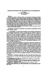
Figures 2(a), 2(b) and 2(c) contain performance profiles over all the 920 runs, excluding cases converging to different critical points, but including failures, like in the tables of results. This choice was done not to handicap BFGS, whose heuristical stopping test may fail to be triggered sometimes. Each line in a performance profile can be interpreted as a cumulative probability distribution of a resource of interest: accuracy, CPU time, (bb) calls. Usually, “smaller” values mean “better performance” of the consider resource. Therefore, for both accuracy and CPU time we plotted the reciprocal of the figures obtained by each solver. In this manner in all the profiles below, the solver with the highest line is the best one for the given indicator of performance. In each profile, we look at the following points: – The leftmost abscissa values, indicating for each solver the percentage of runs for which each solver had the best performance for the given indicator. The highest value corresponds to the best solver. – The abscissa of the intersection between two lines gives the factor that makes the respective solvers comparable. – For an abscissa value θ with ordinate φ(θ), the value 1 − φ(θ) corresponds to the fraction of problems that a solver cannot solve within a factor θ of the best one. The first profile, in Figure 2(a), shows the performance in terms of accuracy. Looking at the highest value for the leftmost abscissa, we conclude that the hybrid variant HyCB is the most precise solver in 72% of the runs. CBun, Hanso, and BFGS are the most accurate solvers in 37%, 36%, 31% runs, respectively. The abscissa values of 2 show that CBun, BFGS and Hanso failed in 34%, 48% and 34% of the runs to achieve half of HyCB’s precision (the respective ordinate values are φ(2) = 0.66, 0.52, 0.66).

19

HyCBf sec 83.64 0.84 5.89 102.08 5350.40 87.44 29.73 1.62 91.74 639.26 15/15

(bb) 1948 435 3207 8860 6657 5193 5251 1374 5836 4307

(a) (reciprocal of) accuracy.

(b) (reciprocal of) CPU time.

(c) (bb) calls.

Figure 2: Performance Profiles.

20

Profile 2(b) measures the performance in terms of CPU time in seconds, and shows that CBun is the fastest solver in 56% of the runs, followed by BFGS, which was fastest in 33% of the runs. At θ = 40, the solvers ordinates are φ(40) = 84, 84, 77, 66. This means that BFGS is as fast as CBun, within a factor of 40, for 84% of the runs, and takes more than 40 times CBun’s CPU time in 16% of the runs. Hanso and HyCB fail to take less than 40 times CBun’s CPU time in 23% and 34% of the runs, respectively. The final profile, in Figure 2(c), measures the performance of the different solvers in terms of (bb) calls, and shows a clear superiority of CBun, which appears as the most economic solver in 80% of the cases. Hanso makes extensive use of (bb) calls, so it should mostly be used for unstructured nonconvex functions that are not too difficult to evaluate (possibly like the matrix problems in [Ska10, Sec. 5.3]). The lines of BFGS and HyCB practically coincide, making both methods indistinguishable in terms of (bb) calls. Since BFGS is faster and HyCB is more precise, the choice between these two solvers should be driven the user’s preference (speed or accuracy), keeping in mind that HyCB is more reliable in terms of stopping test.

6.7

Determining V-dimension

Many composite functions are partly smooth [Lew02], a notion that generalizes to the nonconvex setting the VU-space decomposition for convex functions in [LOS00] and [MS00]. Identification of the VU subspaces can be used to determine directions along which the function behaves smoothly and, hence, identify a region where a Newton-like method is likely to succeed. Such smooth directions lie in the U-subspace; its orthogonal complement, the V-subspace, concentrates all the relevant nonsmoothness of the function, at least locally. Near a critical point x ¯, the V-subpace is spanned ¯ with C ¯ = c(¯ by the subdifferential Dc(¯ x)> ∂h(C), x), and the U-subspace is the orthogonal complement of V. Alternatively, in the wording of [Lew02], the U-subspace is the subspace tanget to the smooth or activity manifold at x ¯, and V = U ⊥ . In [LO08] and [Ska10] it is observed that BFGS can retrieve VU-information by analyzing the eigenvalues of the inverse Hessian used to define a new iterate. For comparison purposes, we consider CBun and BFGS only and estimate the dimension of the respective generated V-subspaces as follows: – For CBun we compute the range of the subspace spanned by the final strongly active gradients in the bundle: n o ˆ ` ) : i ∈ B` with αi` > 0 , dim VCBun := range Dc(xk )> (Gi − G for xk the last generated serious step and ` the iteration triggering the stopping test; recalling that in Step 4 of Algorithm 1 the bundle sizes are kept controlled by a parameter |B max |, – For BFGS we count how many eigenvalues of the final inverse Hessian H cluster near 0:   λi (H) dim VBFGS := card i ≤ n : ≤ , λmax (H) for  a given tolerance.

n dim V CBun BFGS

BadGuy 10 10 10 2.3

10 8 10 8

EucSum 10 10 6 4 8 6 3.8 3.4

10 2 4 2.6

Maxquad 10 3 4 3.2

10 8 8 8

MQ 10 10 6 4 7 4 6.1 5

10 2 3 7

TR48 48 ?? 47 47

Table 6: V dimensions for BadGuy, EucSum, Maxquad, MQ, and TR48. Table 6 reports the obtained results for some of the problems in Group 1 and 2, with low dimension and V-dimensionality depending on the case. The parameters setting were |B max | = 50 and  ∈ {0.1, 0.01} (which gave identical results for this group of runs). Each problem was run 10 times with random starting points. Even though the rules adopted for determining the V-dimensions are rather rough, both CBun and BFGS estimations are reasonable, with a few exceptions. For both solvers the worst results are those obtained for the nonconvex EucSum functions. The extremely low V-dimension estimated by BFGS

21

for BadGuy comes from the fact that it is hard to automatically separate almost null from nonnull, yet small, eigenvalues. An aposteriori (visual) examination of the eigenvalues obtained for each starting point shows a rather erratic behaviour of BFGS for this function over the different starting points, even though BFGS’s heuristic stopping test was always triggered. Such oscillation could be explained by a lack of stability of the Hessian with respect to small perturbations, a common phenomenon for a nonsmooth function near a kink. We made a second group of runs, to determine the impact of smaller or larger V-dimension, with respect to the dimension of the full space. We considered the CPS function, with dimension n ∈ {10, 50, 100} and varying V-dimension. For this example, the V-dimension coincides with the range of the matrix A (taken with sparse density equal to 0.1 for all cases). Table 7 reports the V-dimensions estimated by CBun and BFGS for different parameters. For CBun, the maximum bundle size was set to 50 and 100: we expect results to be worse if |B max | < dim V and the bundle needs to be compressed to an insufficient number of elements. For BFGS, we took two values of , as before. In the table, the parameters appears between parentheses after the name of each solver.

n dim V CBun(50) CBun (100) BFGS10−2 BFGS10−3

10 8 8 8 8 8

10 6 6 6 6.2 6

10 4 4 4 4.4 4

10 2 2 2 2.6 2

50 40 40 40 44 43

50 30 28 30 39.5 37

50 20 20 20 35.5 31

50 10 10 10 35.5 24

50 2 2 2 36 19

CPS 100 90 8 77 95.5 93

100 80 46 78 91 86

100 70 36 70 86.5 81

100 60 44 56 88 80

100 50 44 50 86 75

100 40 30 40 85 71

100 30 29 30 86 67

100 20 20 20 85.5 61

Table 7: V dimensions for CPS. We observe that problems with larger V-subspace are more difficult for both solvers. In general, CBun(100) seems to give a reasonable estimate, but this is not always true, especially when n = 100. We conclude our analysis with Figure 3, with the real and estimated V-dimensions for the 30 different functions, showing that in general BFGS overestimates the size of the V-space. We emphasize that this set of tests determining V-dimensionality is only preliminary, and rather crude. For this reason, the conclusions above should not be taken as an indication of goodness or badness of a solver. The subject of determining VU subspaces is still rather unexplored, with a few exceptions in [LO08], [Ska10], and the MQ functions considered in [DSS09].

Figure 3: True and estimated V-dimensions for the 30 functions.

22

100 10 10 10 86.5 63

100 2 2 2 86 64

Concluding Remarks The composite bundle method presented in this work makes tractable the algorithm ProxDescent in [LW08] for a large class of composite functions, with real-valued, positively homogeneous, and convex outer functions. In particular, the method can be applied to minimize some nonconvex nonsmooth functions, a challenging issue for bundle methods. Our composite cutting-planes model, approximating the conceptual model, avoids typical pitfalls in nonconvex bundle methods (recall Figure 1). The numerical experience reported in this work shows the good performance of the Composite Bundle method for problems of moderate size. For large dimensions, the use of variable prox-metrics may increase the solution times too much, even if there are sparse patterns to exploit. The impact of such increase is problem dependent: for some functions (like CPS and TSP) there is a clear advantage in applying a bundle method (n ≤ 500 in CPS, and n ≤ 3038 in TSP, but Mk ≡ 0). The advantage is less clear for other functions, especially some of the nonconvex ones in Group 3. Since we sometimes also observed that too many short serious steps made CBun stall, we conjecture that a linesearch (replacing or complementing the curved search modifying µ` ) can improve the performance of Algorithm 1 for nonconvex functions, but this is a subject of future research. Although BFGS is accurate and fast (at least for our examples, with blackboxes computationally light), neither BFGS nor Hanso appeared as the best alternatives for many classes of functions considered in our runs. However, conclusions can be different for a different set of test-functions. Also, the usefulness of a solver depends on the specific purpose sought by the user: since BFGS descends fast from a starting point, it could be an interesting alternative if not much accuracy is required, or if the user seeks for a “better” point, without caring if it is the best one. For some problems, we observed that BFGS got stuck at a nonoptimal kink and exited having triggered the heuristical stopping test (the projection of zero on its final bundle was smaller than the tolerance). If reliability is a concern, the output of BFGS can be plugged into a bundle method, as in HyCB, to satisfy a theoretical stopping test. However, if too much accuracy is desired, the hybrid variant is likely to increase the computational bulk of BFGS too much (at least when compared to applying directly CBun). As for Hanso, since it makes extensive use of (bb) calls, we think it should mostly be used for unstructured nonconvex functions that are not too difficult to evaluate (possibly like the matrix problems in [Ska10, Sec. 5.3]). Another important issue to consider for a heavy duty application is that, even in the presence of a composite structure, the resulting smooth mapping may be large, or have no special second order sparse patterns to exploit. In this case, it can be sound to use null or diagonal matrices Mk in Algorithm 1, or apply the limited memory variants in [HMM04] and [Ska10]. We mention the work [KBM10], comparing several NSO general purpose solvers for different type and size of problems, as well as for diferent (bb) available information. Table 3 therein, analizing the efficiency and reliability of the considered solvers, can be useful as a complement of information to the conclusions drawn in our numerical results, keeping in mind that solvers are different and that the test-functions are not exactly the same, although there is some intersection.

Comparison with [NPR08]. The proximity control (nonconvex) bundle algorithm [NPR08] considers models for functions such that several Clarke subgradients at one point can be computed at reasonable cost. The proposed scheme is fairly general and bears some resemblance to our composite approach, which we explain next. Instead of assuming that the objective function enjoys some particular structure, in [NPR08] the authors suppose there is available certain local model, φ(·, xk ), for the objective function f at the current iterate xk . In our notation, f = h ◦ c, and the local model is φ(xk + ·, xk ) = h(ck (·)). As explained in [NPR08, Rems. 2.9 and 6.3], such composite model is both a strong and strict first-order model for f . The local model is approximated by a working model, φk (·, x), which would correspond to our composite ˇ ` (ck (·)). However, in [NPR08, Def. 3.3], the first-order working model satisfies cutting-planes model, h the conditions φk (x, x) = (h ◦ c)(x) and ∂1 φk (x, x) ⊂ ∂1 φ(x, x). For our composite model, this would mean to require that ˇ ` (c(xk )) = (h ◦ c)(xk ) h

and

ˇ ` (c(xk )) = Gi > c(xk )} ⊂ ∂(h ◦ c)(xk ) , conv{Gi for all i ∈ B` : h

which only holds in our case if the outer subgradient information for C = c(xk ) was kept in the bundle.

23

Another related important difference is that when building the working model, in addition to (15), (22), and (23), the method in [NPR08] needs to incorporate certain exact cutting planes. In our setting, an exact cutting plane would correspond to requiring that ∀` ≥ 1, given some γ ∈ ∂(h ◦ c)(xk ),

ˇ ` (ck (·)) . (h ◦ c)(xk ) + γ > · ≤ h

Instead, in (13) we use the outer subgradient Γ` ∈ ∂h(C ` ) for C ` = c(xk +d` ) to detect if the linearization of the inner mapping is not good enough and trigger the backtracking process. But if xk + d` is declared a serious step, the corresponding subgradient Γ` does not enter the bundle (nothing prevents the bundle management step to incorporate this data, though). Like ours, the quadratic programming subproblem in [NPR08] includes a second-order term with a possibly nonpositive definite matrix Mk , augmented by a (positive enough) matrix µ` I. But the acceptance test corresponding to (12) uses a predicted decrease that is different from ours. Namely, instead of δ` in (11), the larger amount δ`0 := δ` + 12 µ` d` > d` is used. As for null steps, the decision on whether or not to increase the parameter µ` is done by checking if, for some parameter m3 ∈ (m1 , 1), h(c(xk ) + Dk d` ) ≤ (h ◦ c)(xk ) − m3 δ`0 (the prox-parameter is left unchanged if the inequality above does not hold). Convergence results for the proximity control bundle method with strong first-order models are similar to ours. The method keeps matrices Mk bounded below and above by ±qI for some 0 < q < +∞, so (18) always holds. The case of infinite null steps is treated in [NPR08, Lem. 4.1], where it is shown that a subsequence of the prox-parameter diverges and, hence, checking satisfaction of our condition (24) is not straightforward. Section 7 in [NPR08], devoted to applications, contains several cases showing the good numerical behaviour of the algorithm. An interesting subject of future research would be to compare both algorithms performance on composite objective functions.

References [BF95]

J. V. Burke and M. C. Ferris, A Gauss-Newton method for convex composite optimization, Mathematical Programming 71 (1995), 179–194.

[BGLS03] J.F. Bonnans, J.Ch. Gilbert, C. Lemar´echal, and C. Sagastiz´ abal, Numerical optimization. theoretical and practical aspects, Universitext, Springer-Verlag, Berlin, 2003, xiv+423 pp. [BLO02]

J.V. Burke, A. Lewis, and M. Overton, Two numerical methods for optimizing matrix stability, Linear Algebra and its Applications 351-352 (2002), 117–145.

[BS00]

J. F. Bonnans and A. Shapiro, Perturbation analysis of optimization problems, Springer Series in Operations Research, Springer-Verlag, New York, 2000.

[CL93]

R. Correa and C. Lemar´echal, Convergence of some algorithms for convex minimization, Math. Program. 62 (1993), no. 2, 261–275.

[DSS09]

Aris Daniilidis, Claudia Sagastiz´ abal, and Mikhail Solodov, Identifying structure of nonsmooth convex functions by the bundle technique, SIAM Journal on Optimization 20 (2009), no. 2, 820–840.

[ES10]

G. Emiel and C. Sagastiz´ abal, Incremental-like bundle methods with application to energy planning, Computational Optimization and Applications 46 (2010), 305–332.

[Fle87]

R. Fletcher, Practical methods of optimization (second edition), John Wiley & Sons, Chichester, 1987.

[Har03]

W.L. Hare, Nonsmoth Optimization with Smooth Substructure, Ph.D. thesis, Department of Mathematics, Simon Fraser University, 2003.

[HMM04] M. Haarala, K. Miettinen, and M. M. Makela, New limited memory bundle method for largescale nonsmooth optimization, Optimization Methods and Software (2004), no. 6, 673–692. [HS10]

Warren Hare and Claudia Sagastiz´ abal, A redistributed proximal bundle method for nonconvex optimization, SIAM Journal on Optimization 20 (2010), no. 5, 2442–2473.

24

[HUL93]

J.-B. Hiriart-Urruty and C. Lemar´echal, Convex analysis and minimization algorithms, Grund. der math. Wiss, no. 305-306, Springer-Verlag, 1993, (two volumes). [HUL01] J.-B. Hiriart-Urruty and C. Lemar´echal, Fundamentals of convex analysis, Grundlehren Text Editions, Springer-Verlag, Berlin, 2001. [KBM10] N. Karmitsa, A. Bagirov, and M. M. Makela, Comparing different nonsmooth minimization methods and software, Optimization Methods and Software (2010). [Kiw86] K.C. Kiwiel, A method for solving certain quadratic programming problems arising in nonsmooth optimization, IMA Journal of Numerical Analysis 6 (1986), 137–152. [Lew02] A.S. Lewis, Active sets, nonsmoothness and sensitivity, SIAM Journal on Optimization 13 (2002), no. 3, 702–725. [LO08] Adrian S. Lewis and Michael L. Overton, Nonsmooth Optimization via BFGS, Avalaible at http://www.optimization-online.org/DB_HTML/2008/12/2172.html., 2008. [LOS00] C. Lemar´echal, F. Oustry, and C. Sagastiz´ abal, The U-Lagrangian of a convex function, Trans. Amer. Math. Soc. 352 (2000), no. 2, 711–729. [LS97] C. Lemar´echal and C. Sagastiz´ abal, Practical aspects of the Moreau-Yosida regularization: theoretical preliminaries, SIAM Journal on Optimization 7 (1997), no. 2, 367–385. [LV00] L. Luksan and J. Vlcek, Test problems for nonsmooth unconstrained and linearly constrained optimization, Tech. Report 798, Institute of Computer Science, Academy of Sciences of the Czech Republic, 2000. [LW02] Chong Li and Xinghua Wang, On convergence of the gauss-newton method for convex composite optimization, Mathematical Programming 91 (2002), 349–356, 10.1007/s101070100249. [LW08] A.S. Lewis and S.J. Wright, A proximal method for composite minimization, Available at http://www.optimization-online.org/DB_HTML/2008/12/2162.html, 2008. [Mif77] R. Mifflin, Semi-smooth and semi-convex functions in constrained optimization, SIAM Journal on Control and Optimization 15 (1977), 959–972. [MS00] R. Mifflin and C. Sagastiz´ abal, On VU-theory for functions with primal-dual gradient structure, SIAM Journal on Optimization 11 (2000), no. 2, 547–571. [MS03] , Primal-Dual Gradient Structured Functions: second-order results; links to epiderivatives and partly smooth functions, SIAM Journal on Optimization 13 (2003), no. 4, 1174–1194. [MS04] , VU-Smoothness and Proximal Point Results for Some Nonconvex Functions, Optimization Methods and Software 19 (2004), no. 5, 463–478. , A VU -algorithm for convex minimization, Math. Program., Ser. A 104 (2005), no. 2– [MS05] 3, 583–608. [Nes07] Y. Nesterov, Gradient methods for minimizing composite objective functions, Discussion paper 2007/76, CORE, 2007, Avalaible at http://www.optimization-online.org/DB_HTML/2007/ 09/1784.html. [NPR08] D. Noll, O. Prot, and A. Rondepierre, A proximity control algorithm to minimize nonsmooth and nonconvex functions, Pac. J. Optim. 4 (2008), no. 3, 569 – 602. [NY83] A. Nemirovsky and D. Yudin, Problem complexity and method efficiency in optimization, A Wiley-Interscience Publication, John Wiley & Sons Inc., New York, 1983. [Ous00] F. Oustry, A second-order bundle method to minimize the maximum eigenvalue function, Math. Program. 89 (2000), no. 1, Ser. A, 1–33. [RW98] R.T. Rockafellar and R.J.-B. Wets, Variational analysis, Grund. der math. Wiss, no. 317, Springer-Verlag, 1998. [Sha03] A. Shapiro, On a class of nonsmooth composite functions, Math. Oper. Res. 28 (2003), no. 4, 677–692. [Ska10] Anders Skajaa, Limited Memory BFGS for Nonsmooth Optimization, Master’s thesis, Courant Institute of Mathematical Science, 2010. Appendix with full tables

25

26 1: problems in Table 1. Table 8: Results for Group

(10)

(10)

mean,

(10)

1-48

1-29

(30)

5-30

3-20

(100)

max/fails

MEAN,

max/fails

mean,

Ury

1-10

max/fails

mean,

TSP

sec,

CBunf (bb) RA, sec,

CBunm (bb) RA,

10/10

0/0

0/0

10,

11, 12, 10, 11,

1/1

1/1

0/0

384 8, 415 13, 285 7, 362 9,

50/50

83, 627 10,

30/30

18 0, 66.20, 39 0,175.27, 77 -1,199.46, 45 -0,146.98,

22, 262 4,

0/0

0.18, 1.08, 4.20, 1.82,

(bb) RA,

(bb) RA,

0/1

0.77, 441 8, 0.77, 441 8,

0/0

1.94, 289 9, 1.94, 289 9,

sec,

BFGSm (bb) RA,

0/0

0.32, 683 8, 0.32, 683 8,

0/0

2.53, 377 9, 2.53, 377 9,

sec,

Hansof (bb) RA,

0/1

1.66, 1451 12, 1.66, 1451 12,

0/0

2.52, 378 9, 2.52, 378 9,

sec,

Hansom (bb) RA, sec,

HyCBm (bb)

0/0

0.24, 443 12, 0.24, 443 12,

0/0

0/0

0.84, 452 0.84, 452

10/10

2.00, 301 9, 22.12, 1793 2.00, 301 9, 22.12, 1793

sec,

HyCBf

0/10

0/10

0/10

0/10

0/0

4/4

32.57, 2738 13, 46.02, 2738 13, 290.53,29439 13, 232.43,20537 15, 33.16, 2746 13, 115.59, 2816 32.57, 2738 13, 46.02, 2738 13, 290.53,29439 13, 232.43,20537 15, 33.16, 2746 13, 115.59, 2816

0/1

0.20, 432 8, 0.20, 432 8,

0/0

1.92, 289 9, 1.92, 289 9,

sec,

BFGSf

3/38

2/6

0/6

0/6

3/46

402, 2646 11,

1/29

0/38

460,13262 11,

0/22

0/46

453,10166 13,

0/29

578 14, 3.40, 823 14, 7.39, 9855 14, 6.60, 3932 16, 1395 13, 10.13, 1395 13, 20.29,19696 13, 25.20, 8770 14, 2433 7, 41.38, 2503 7, 32.42,23734 7, 82.82,18543 16, 1469 11, 18.30, 1574 11, 20.03,17762 11, 38.20,10415 15,

397, 2623 11,

1/21

0.51, 2.12, 5.29, 2.64,

2/6

584 14, 1401 16, 2440 12, 1475 14,

0/0

411, 2730 12,

0/0

0.53, 2.18, 5.44, 2.72,

0/0

961 1430 2635 1675

20/20

438, 3080

6/6

13.20, 14.59, 84.60, 37.46,

0/0

6, 9.68, 608 9, 0.12, 173 9, 0.09, 173 9, 0.20, 319 9, 0.19, 313 9, 0.12, 180 9, 0.10, 180 7, 20.30,1000 16, 60.39, 5145 16, 68.11, 5145 16, 217.17,44446 16, 241.89,44446 16, 66.89, 5660 16, 77.13, 5664 6, 83.85,1363 16, 352.03, 5657 16, 360.70, 5657 16, 352.03, 5657 16, 360.70, 5657 16, 374.85, 6202 16, 391.58, 6216 4,330.90,1092 10,7375.32,21777 10,7352.68,21777 10,7375.33,21777 10,7352.68,21777 16,7617.81,22701 11,7586.84,22592 6,111.18,1016 13,1946.97, 8188 13,1945.40, 8188 13,1986.19,18050 13,1988.87,18048 14,2014.92, 8686 13,2013.91, 8663

10/10

12, 3.51, 48 3,133.67, 196 13, 12, 3.51, 48 3,133.67, 196 13,

0/0

11, 0.16, 40 11, 1.20, 62 8, 11, 0.16, 40 11, 1.20, 62 8,

0/0

8, 1.70, 135 1, 24.32,1501 9, 8, 1.70, 135 1, 24.32,1501 9,

RA,

16, 0.11, 50 2-442 7, 13.38, 996 3-1173 6, 91.09,2044 4-3038 4,303.63,1090 (40) 8,102.05,1045

max/fails

mean,

TR48

max/fails

1-10

MQ

max/fails

mean,

BadGuy 1-10

(bb) #-n

Name CPS cvx MQ cvx EucSum ncv ncv ncv ncv ncv ncv ncv TiltedNorm cvx GenModRos ncv ModRos ncv NesChebRos ncv Ferrier ncv NK ncv cvx/ncv LV ncv ncv ncv ncv ncv ncv ncv Ury ncv ncv ncv cvx ncv

h◦c 0 (opt)

Parameters n ∈ {10, 50, 100, 500} range A ∈ {0.2, 0.8}n n ∈ {10, 50, 100, 500} range A ∈ {0.2, 0.8}n m = range A + 3

0 (opt)

n = 4, range A = 2 n = 10, range A = 8 n = 10, range A = 2 n = 50, range A = 40 n = 50, range A = 10 n = 100, range A = 80 n = 100, range A = 20 n ∈ {10, 50, 100, 500} w=4 n = 12 U = 1, V = 10 n=2 w ∈ {1, 2, 4, 8} n ∈ {5, 10, 50, 100} x0 ∈ [0, 2] n ∈ {10, 50, 100} case ∈ {1, 3}

0.930538450443740 0.465587005455171 0.666424291184390 0.399571129728750 0.002143493387185 excluded 0.333869560359649 0 (opt)

(best) (best) (best) (best) (best) (best)

5.377690121369670 (best) 0 (opt) 0 (opt) 0 (opt)

case = 8 case ∈ {1, 3, 4, 5, 9}

excluded √ {0, − 2(n − 1), 2(n − 1), 2(n − 1), 0} (opt)

case = 3, n ∈ {10, 50, 100, 500} case = 4, n = 10 case = 4, n = 50 case = 4, n = 100 case = 4, n = 500 case ∈ {5, 6}, n ≤ 100 case ∈ {5, 6}, n = 500

excluded 106.059118520625645 (best) 587.997761620671213 (best) 1190.421065495747825 (best) 6009.807496496680869 (best) 0 (best) (excluded)

n = 10, cubic=0.01 n = 20, cubic=0.01 n = 30, cubic=0.01 n = 100, cubic=0 n = 100, cubic=0.01

500 (best) 909.889558838787480 (best) 1114.734712066170232 (best) 1159.869805021747879 (best) 1162.455887489049701 (best)

Table 10: Optimal (opt) or best (best) function values, for problems in Groups 2 and 3.

27

(bb)

#-n 12 12 11 6 6 10 10

CBunf sec 0.07 0.03 0.02 0.07 0.08 0.07 0.06

(bb) 14 14 8 9 9 8 10

RA

7 7 6 5 6 6 6

BFGSf sec 0.07 0.05 0.04 0.51 0.39 0.27 0.22

10 7 16 5 6 9

0.34 0.09 0.01 3.02 0.13 0.72

9 27 6 30 11 17

6 7 5 6 7 6

0.08 0.21 0.02 3.35 0.34 0.80

8 7 5 5 6

0.04 0.02 0.26 1.51 0.46

8 9 13 53 21

4 4 2 4 4

0.11 0.03 1.65 0.39 0.55

9 1.93 1050 6 2.19 1229 16 0.43 237 6= stationary points 6= stationary points 10 1.52 839

7 8 9

8

RA 1-10 2-10

CPS

3-10 4-50 5-50 6-50

mean, max/fails

(60)

0/0 1-4 2-10

EucSum

3-10 4-50 5-50

mean, max/fails

(50)

Ferrier

2-10 3-50 4-50

mean, max/fails

(40)

2-12

GenModRos

3-12 4-12 5-12

mean, max/fails

(30) 1-10 2-10 3-10

LV

4-10 5-50 6-50 7-50 8-50

mean, max/fails

(60)

MQ

3-10 4-50 5-50

mean, max/fails

(40)

ModRos

2-2 3-2 4-2

mean, max/fails

(40)

10-50 11-50 12-50 2-10

NK

3-10 4-10 5-10 6-10 7-50 8-50 9-50

mean, max/fails

(100)

NesChebRos

2-10 3-50

mean, max/fails

(30)

TiltedMax

2-20 3-50

0.12 0.05 1.76 0.46 0.60

1.10 0.83 1.03

2044 1568 1850

16 16 10

0.35 0.32 0.26

547 503 492

0.99

1821

14

0.31

514

0.16 0.11 2.76 0.69 0.93

0.24 0.21 0.24

489 447 480

7 8 9

0.23

472

8

0/0

0/0

0/0

148 147 1874 965 783

0/0

0/0

0/0

1.52 0.29 0.24

2639 479 453

16 6 7

0.18 0.11 0.16

351 209 311

16 16 16 11

5.16 2.07 3.84 1.91

2534 1582 2778 1292

16 16 16 11

42.32 2.33 4.10 8.47

29835 1764 2960 6355

16 16 16 13

5.22 2.11 3.88 1.94

2539 1586 2783 1297

13 10 11 8 11

8 7 4 8 7

0.30 0.04 13.74 1.08 3.79

680 144 5769 2256 2212

9 7 4 8 7

1.66 0.07 76.94 1.31 20.00

3755 205 31841 2642 9611

10 10 8 9 9

0.32 0.05 14.11 1.13 3.90

38 53 150 278 130

6 6 6 5 6

0.02 0.02 0.03 0.06 0.03

37 56 109 214 104

6 6 6 5 6

0.03 0.03 0.03 0.07 0.04

68 80 122 228 124

10 10 9 6 9

0.04 0.06 0.27 0.30 0.17

9 0.10 32 16 0.55 23 6= stationary points 16 0.11 8 16 0.30 82 13 0.05 12 14 0.09 31 6= stationary points 11 0.03 12 8 0.44 22 5 3.01 44 6 0.45 11 11 0.51 28

6 8

0.03 0.06

63 75

6 8

0.07 0.20

126 298

16 11

0.08 0.17

81 79

5 6 6 7

0.04 0.07 0.07 0.02

72 191 199 70

5 7 6 7

0.15 0.17 0.34 0.06

269 408 741 140

10 9 16 16

0.13 0.32 0.09 0.05

76 237 205 77

5 5 16 16 8

0.02 0.09 3.14 3.79 0.73

76 238 2351 2438 577

5 5 16 16 8

0.06 0.18 23.55 36.04 6.08

141 431 29652 29739 6195

16 16 16 16 14

0.06 0.43 3.32 3.98 0.86

88 251 2357 2443 589

188 9 14 71

1 2 1 1

0.16 0.08 1.87 0.70

415 184 1727 775

2 2 1 2

0.58 0.15 25.59 8.77

1886 398 28720 10335

2 2 1 2

0.45 1.09 1.91 1.15

30 46 109

6 7 7

0.05 0.09 0.22

180 358 763

6 7 7

0.13 0.30 0.60

10 10 7 9 9

0.06 0.02 0.44 0.06 0.14

9 7 4 2 6

0.07 0.04 0.13 0.24 0.12

0/10

16 16 16 16

0.36 0.02 0.21 0.20

14 13 6

0.10 0.25 2.63

0/10

7/20

67 100 382 492 260

17/17

0/19

2/3

687 147 5775 2259 2217

0/0

0/0

0/19

28

0/0

0/10

0/0

3/3 1-10

7 9 6 5 7

4 5 2 5 4

43 601 77 1416 754 578

8 5 5

0/0 1-5

254 348 4820 1678 1775

142 141 1865 961 777

0/0

347 206 305

13/13 1-10

0.10 0.25 0.03 3.49 0.36 0.85

0.17 0.09 0.15

0/0 1-2

16 16 5 16 16 14

0/0

(bb) 187 134 98 774 563 352 352

8 5 4

10/10 2-10

65 15622 143 1626 1085 3708

0.12 6.36 0.06 3.79 0.50 2.17

0/0

6= stationary points 4 4.70 1740 16 0.02 8 16 0.03 15 6= stationary points 3 1.89 149 3 1.21 55 5 0.65 34 8 1.42 334

8 9 9 5 10 9 8

HyCBf sec 0.09 0.06 0.05 0.54 0.42 0.29 0.24

6 7 5 6 7 6

0/5

2/2

RA

40 590 75 1411 752 574

7 7 6 5 6 6 6

0/0

0/0 1-12

(bb) 245 196 156 953 741 530 470

RA

0/0

1/1 1-10

Hansof sec 0.11 0.09 0.07 0.65 0.53 0.41 0.31

(bb) 184 131 94 772 560 349 348

1/1

0/2

614 716 1732 1021

5/5

407 15 1043 9 1946 7 Continued

0.07 0.12 0.24 on next

186 365 766 page

(30)

11

Table 11 – continued from previous page CBunf BFGSf Hansof sec (bb) RA sec (bb) RA sec 0.99 62 7 0.12 434 7 0.35

2-10

(30)

16 11 10 12

0.18 1.01 4.66 1.95

(510)

10

0.73

#-n

(bb)

RA

mean, max/fails

0/0

Ury

4-20 6-30

mean, max/fails MEAN, max/fails

0/0

20 42 110 58

7 11 16 11

0.29 1.90 5.81 2.67

143

7

1.07

0/0

RA

10

HyCBf sec 0.14

14847 19606 23928 19460

10 16 16 14

0.30 2.06 6.61 2.99

5544

10

1.20

0/0

399 1305 2627 1444

7 11 16 11

10.16 18.19 30.98 19.78

819

7

6.17

0/19

29/29

(bb) 1132

0/0

0/19

9/76

(bb) 439 405 1316 2649 1456

0/0

0/60

864

23/23

Table 11: Results for Group 2: problems in Table 3, n ≤ 50.

(bb)

#-n RA 10-500 11-500

CPS

12-500 7-100 8-100 9-100

mean, max/fails EucSum mean, max/fails Ferrier mean, max/fails

(60)

7-100

(10)

6-100

(20)

13-500 14-500 15-500 16-500 9-100

(40)

7-100 8-500 9-500

(40)

14-100 15-100 16-100 17-100 18-100 19-500 20-500 21-500 22-500 23-500 24-500

mean, max/fails NesChebRos mean, max/fails TiltedMax mean, max/fails Ury

5 5

0.88 12.20 6.54

(100)

(10)

(10)

8-100

0.78 0.78

Hansof sec 227.11 238.07 160.79 5.95 4.85 2.95 106.62

(bb) 6780 4515 2312 1765 1306 870 2925

RA

3 8 9 5 9 10 7

0/0

433 433

5 5

1.08 1.08

4657 1748 3203

14 5 10

15.64 3.18 9.41

HyCBf sec 106.60 230.25 152.93 5.33 4.34 2.36 83.64

(bb) 2410 4217 2014 1466 1008 572 1948

0/0

734 734

6 6

17958 2916 10437

14 5 10

9.16 2.62 5.89

0/0

0.84 0.84

435 435

0/0

9.07 2.58 5.83

3 0.54 13 3 5.44 113 4 5.65 121 6= stationary points 4 4.25 13 6= stationary points 6= stationary points 6= stationary points 4 3.97 65

16 16 4

22.09 17.69 29.24

4676 3676 5882

16 16 16

112.32 18.38 40.52

43976 3978 10822

16 16 5

22.17 17.81 29.49

4679 3680 5887

16

338.32

21189

16

757.08

60490

16

338.82

21191

13

101.84

8856

16

232.08

29816

13

102.08

8860

0/2

2 16 -0 0 4

90.94 0.15 5023.56 478.97 1398.41

105 9 22 25 40

4 5 0 3 3

16 1.35 23 4 7.81 36 5 0.91 9 12 0.88 21 6= stationary points 10 0.21 8 5 19.78 39 2 11.11 7 6 16.54 18 16 5.44 22 6= stationary points 16 0.83 7 9 6.49 19

5 16 16 8

16 16

0.84 0.84

3 3

7.84 7.84

1 0

70.85 25.19

0/0

1/5

165.89 12.16 14634.68 991.68 3951.10

16 5 0 16 9

0.63 13.09 16.35 0.13

410 4443 4752 83

5 16 16 8

4 4 16 16 8

0.09 30.79 342.25 451.70 2.25

69 902 19620 21468 68

5 10

2.16 85.94

19 19

1 1

29.63 29.63

105 105

7 7

1.59 1.59

94 91

7 16

61.95 61.52

5 6 16 3 8

0.80 58.45 79.97 0.39

711 43744 44052 384

5 16 16 16

0.80 13.41 16.86 0.26

413 4447 4756 86

4 4 16 16 8

0.29 32.57 763.23 1006.16 6.47

370 1204 58920 60769 489

16 16 16 16 11

0.31 39.20 343.85 453.87 3.20

75 920 19621 21470 72

72 5189

5 10

4.41 195.28

373 21102

8 14

2.64 87.44

74 5193

5247 5247

1 1

112.88 112.88

44548 44548

1 1

29.73 29.73

1372 1372

7 7

2.04 2.04

2776 2776

7 7

5854 5685

7 16

269.76 277.93

0/5

0/8

6544 5125 8384 6575 6657

0/0

0/10

0/0

172.30 12.27 20200.74 1016.28 5350.40 2/2

0/8

0/10

29

0/0

42648 6178 42086 42461 33343

6/8

804.07 13.23 75735.20 5382.02 20483.63

4661 1752 3207

0/0

0/4

6536 5122 8352 6572 6646

2/2 7-100

3 5 5 5 5 6 5

0/0

0/0 4-100

RA

14 5 10

0/0 4-100

(bb) 2409 4214 2011 1464 1005 569 1945

14 114 64

6/6 13-100

NK

5 4 4

BFGSf sec 106.27 229.58 152.19 5.27 4.26 2.29 83.31 0/0

6= stationary points 16 0.27 8 16 0.27 8

0/0 6-100

mean, max/fails

3 5 5 5 5 6 5

1/1

12-100

MQ

RA

0/0 5-100

11-100

mean, max/fails

(bb) 7 7 7 7 8 8 7

0/0 6-100

10-100

LV

6 5 5 6 6 6 6

CBunf sec 1.31 1.26 1.25 0.13 0.14 0.14 0.70

5251 5251

0/0

0/0

1.62 1.62

1374 1374

0/0

45155 44986

16 95.00 5897 16 88.49 5774 Continued on next page

(bb)

#-n (20)

0

CBunf sec 48.02

(310)

7

163.67

RA

mean, max/fails MEAN, max/fails

Table 12 – continued from previous page BFGSf Hansof (bb) RA sec (bb) RA sec 92 12 61.73 5770 12 273.85

20/20 29/29

14/20

47

7

480.19 21/53

(bb) 45070

RA

16

HyCBf sec 91.74

21195

9

639.26

0/20

4295

8

2379.65

13/13

0/47

Table 12: Results for Group 3: problems in Table 3, n = 100 and n = 500.

30

(bb) 5836

15/15

4307