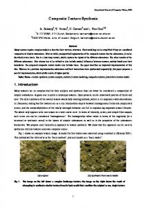
synthesize such âcomposite texturesâ, where the layout of the different subtextures is itself modeled as a texture, which can be generated automatically.
Composite Texture Descriptions Alexey Zalesny1, Vittorio Ferrari1, Geert Caenen2, Dominik Auf der Maur1, and Luc Van Gool1, 2 1 Swiss Federal Institute of Technology Zurich, Switzerland {zalesny, ferrari, aufdermaur, vangool}@vision.ee.ethz.ch http://www.vision.ee.ethz.ch/~zales 2 Catholic University of Leuven, Belgium {Geert.Caenen, Luc.VanGool}@esat.kuleuven.ac.be
Abstract. Textures can often more easily be described as a composition of subtextures than as a single texture. The paper proposes a way to model and synthesize such “composite textures”, where the layout of the different subtextures is itself modeled as a texture, which can be generated automatically. Examples are shown for building materials with an intricate structure and for the automatic creation of landscape textures. First, a model of the composite texture is generated. This procedure comprises manual or unsupervised texture segmentation to learn the spatial layout of the composite texture and the extraction of models for each of the subtextures. Synthesis of a composite texture includes the generation of a layout texture, which is subsequently filled in with the appropriate subtextures. This scheme is refined further by also including interactions between neighboring subtextures.
1
Composite Textures, Divide and Conquer
Natural textures can be of a very high complexity, which renders them difficult to emulate by texture synthesis methods. Many of such textures consist of patches, which in turn contain patterns of their own. Good examples are the textures of building materials like marbles or limestones, or the textures of different landscape types. A countryside texture could, e.g. be a mixture of meadows and forests. We will refer to such textures as composite textures. Whereas the patterns within the patches may already be homogeneous enough to be modeled and synthesized successfully with existing techniques, modeling and synthesizing the mixture directly tends to be less effective. It therefore stands to reason to divide the synthesis of composite textures into several steps: 1. Segment (by hand or otherwise) example image(s) of the composite texture to be modeled, where each class is given its own label. 2. Consider the resulting label map (with labels assigned to all pixels) as a texture and extract a model for it. 3. Also extract models for the textures corresponding to the different labels (i.e. the different classes/segments). 4. Generate a synthetic label map, based on the model of step 2. 5. Fill in the segments generated under step 4 with textures according to their labels,
based on the models of step 3. This scheme tallies with ideas about “macrotextures” vs. “microtextures” that have emerged as soon as texture research started in computer vision. The label map can be considered a macrotexture, whereas the textures within the segments of constant label values would be microtextures. In this paper, we will refer to the macrotextures as “label textures”, and to the microtextures as “subtextures”. Although such ideas have been around for quite a while, it seems that so far such hierarchical approach has not really been implemented for textures of a strong stochastic nature. When ideas about hierarchical analysis are used, it is usually in the context of multi-resolution schemes, which have contributed greatly to the state-ofthe-art in texture synthesis (see e.g. [2, 7] as seminal examples). Contributions that come closest to the work presented here have used label textures that were handdrawn by the user and the corresponding textures were then filled in with texture either by “smart copying” from example [8] or by synthesis techniques [13]. The composite texture approach as just described does not include mutual influences between the subtextures. It is not exceptional that the subtextures are not completely stationary within their domains. In particular, regularly a kind of transition zone is found near their boundaries. These changes may well depend on the texture on the other side of the boundary. Later in the paper we will modify the composite texture scheme to include such effects. The remainder of the paper is organized as follows. Section 2 describes the texture synthesis approach used to generate the label textures and the subtextures. Section 3 shows some results for the synthesis of composite textures. Section 4 describes the inclusion of subtexture interactions (nonstationary aspects). Section 5 concludes the paper.
2
Image-Based Texture Synthesis
This section describes the approach that we use to synthesize the textures, i.e. both the label textures and the subtextures. More information about this texture modeling and synthesis approach can be found in [13]. It follows the cooccurrence paradigm in that texture is synthesized as to mimic the pairwise statistics of the example texture. This means that the joint probabilities of the intensities at pixel pairs with a fixed relative position are approximated. Such pairs will be referred to as cliques, and pairs of the same type (same relative position between the pixels) as clique types. This is illustrated in Fig. 1.
Fig. 1. Dots represent pixels. Pixels connected by lines represent cliques. Left: cliques of the same type, right: cliques of different types.
The texture model consists of statistics for a selected set of clique types. Clique type selection follows an iterative approach, where clique types are added one by one
to the texture model, a texture synthesized based on the model is each time updated accordingly, and the statistical difference between the example texture and the synthesized texture is analyzed to decide which further clique type addition to make. The set of selected clique types is called the neighborhood system. The complete texture model consists of this neighborhood system and the statistical parameter set. The latter contains the histograms of intensity differences between the two pixels of all cliques of the same type. A sketch of the texture model extraction algorithm is as follows: step 1: Collect the complete 2nd-order statistics for the example texture, i.e. the statistics of all clique types. After this step the example texture is no longer needed. As a matter of fact, the current implementation focuses on clique types up to a maximal length. step 2: Generate an image filled with independent noise and with values uniformly distributed in the range of the example texture. This noise image serves as the initial synthesized texture, to be refined in subsequent steps. step 3: Collect the statistics for all clique types from the current synthesized image. step 4: For each clique type, compare the intensity difference histograms of the example texture and the synthesized texture and calculate their Euclidean distance. In fact, the intensity histograms pure (singletons) are considered as well. step 5: Select the clique type with the maximal distance (see step 4). If this distance is less than a threshold, then leave the algorithm with the current model. Otherwise add the clique type to the current (initially empty) neighborhood system and all its statistical characteristics to the current (initially empty) statistical parameter set. step 6: Synthesize a new texture using the updated neighborhood system and texture parameter set. step 7: Go to step 3. After running this algorithm we have the final neighborhood system of the texture and its statistical parameter set. A more detailed description of this texture modeling approach is given elsewhere [13]. In that paper it is also explained how the synthesis step works and how we generalize this texture modeling to colored textures. The proposed algorithm produces texture models that are very small compared to the complete 2nd-order statistics extracted in step 1 and also compared to the example image. Typically only 10 to 40 clique types are included and the model amounts from a few hundred to a few thousand bytes. Another advantage is that the method avoids verbatim copying of parts of the example images. This is an advantage that it shares with similar approaches [5, 6, 9, 12]. Verbatim copying becomes particularly salient when large patches of texture need to be created, e.g. when covering a large wall with a marble texture. Then the repeated appearance of the same structures quickly becomes salient to the human eye. For the texture mapping on such large surfaces this problem is more serious than may transpire from state-of-the-art publications that suffer from this problem (e.g. [3, 11]), as the extent of the textures that can be shown in papers is rather small. The basic texture synthesis approach described in this section can handle quite
broad classes of textures. Nevertheless, it has problems with the composite type of textures considered here. Comparisons between single and composite texture synthesis results will be shown later.
3
The Segmentation of Composite Textures
The steps of the composite texture modeling scheme proposed in section 1 are illustrated on the basis of a few examples. Fig. 2 shows a modern “thorn-cushion steppe” type of landscape (left). It consists of several ground cover types, like “rock”, “green bush”, “sand”, etc., for which the corresponding segments are drawn in the figure on the right.
Fig. 2. Left: an example of “thorn-cushion steppe”, Right: manual segmentation into basic ground cover types (also see Fig. 4).
If one were to directly model this composite ground cover as a single texture, the basic texture analysis and synthesis algorithm proposed in the last section would not be able to capture all the complexity in such a scene. Fig. 3 shows the result of such synthesis.
Fig. 3.
Attempt to directly model the scene in Fig. 2 as a single texture.
In keeping with the composite texture scheme of section 1, an example image like this is first decomposed into different subtextures, as shown in Fig. 2 (right). The segments that correspond with different subtextures have been given the same
intensity (i.e. the same label). This segmentation has been done manually. Fig. 4 shows the image patterns corresponding to the different segments. The textures within the different segments are simple enough to be handled by the basic algorithm. Hence, in this case 6 subtexture models are created, one for each of the ground cover types (see caption of Fig. 4). But also the map with segment labels (Fig. 2 right image) can again be considered to be a texture, describing a typical landscape layout in this case. This label texture is quite simple again, and can be modeled by the basic algorithm of section 2. Hence, similar label textures can be generated automatically as well. The synthesis of this composite texture first generates a landscape layout as a label texture. Subsequently, the different segments are filled in with the corresponding subtextures, based on their models. As an alternative, a graphical designer or artist can draw the layout, after which the computer fills in the subtextures in the segments that s/he has defined, according to their labels. Fig. 5 shows one example for both procedures.
Fig. 4. Manual segmentation of the terrain texture shown in Fig. 2. Left: segments corresponding to 1-green bush, 2-rock, 3-grass, 4-sand, 5-yellow bush. Right: left-over regions are grouped into an additional mixed class.
Fig. 5. Synthetically generated landscape textures. Left: based on a manually drawn label texture. Right: based on an automatically generated label texture.
Note that except for the hand segmentation of the label texture in Fig. 2, the right image has been created fully automatically and arbitrary amounts of such texture can be generated, enough to cover a terrain model with never-repeating, yet detailed texture. As mentioned before, the fact that this approach doesn’t use verbatim copying of parts in the example images has the advantage that no disturbing repetitions are created. A complete automation of the composite texture scheme would have to include an initial, unsupervised segmentation of the scene, so that no hand segmented label texture is needed. Such unsupervised segmentation is not an easy matter of course, but in certain cases may nevertheless be possible. As Paget [10] noticed, the optimal complexity of texture models for segmentation is typically lower than that required for synthesis. This can be key to avoiding a chicken-and-egg situation with such fully automated process. In case the features needed for the segmentation were of the same complexity as the models that we extract from segmented data, the whole procedure can no longer run automatically. Fig. 6 left shows two images that could be segmented automatically. As a matter of fact, truly textural features were not needed at all in this case. Segmentation based on Lab color data was sufficient. The data around each pixel were smoothed with a Gaussian filter of size 5x5. Each pixel is described by a three dimensional color feature vector. For more general case, an additional vector is built of simple texture features, obtained as the outputs of a bank of simple filters. A cosine metric between such feature vectors is used as similarity measure between pairs of pixels (Bhattacharyya distance). A sample pixel set is drawn from the image and a complete graph is constructed where vertices correspond to pixels and edges are weighted by the similarity measure. The graph is then partitioned into completely connected, disjoint subsets of vertices so as to maximize the total sum of the similarities over all remaining edges. These subsets are also referred to as “cliques”, but this time in the graph theoretical sense. The pixels in each subset now represents a subtexture. This robust segmentation procedure is efficiently obtained via the Clique Partitioning approximation algorithm of [4]. It is worth noting that the algorithm is completely unsupervised: it doesn’t need to know the number of subtexture classes, their size, or any information other than the image data itself. The segmentation results for the two images are shown in Fig. 6 right. A more detailed description of the unsupervised segmentation scheme is given elsewhere [1]. Fig. 7 shows the result of a fully automatic composite texture synthesis for the top texture of Fig. 6. No user input whatsoever was needed to generate this result. Fig. 7 right is the label texture that was generated. Automatic segmentation of a composite texture will not always be possible or even desirable. Fig. 8 shows one of the more complicated types of limestones that was used as building material at the ancient city of Sagalassos in Turkey, now a center of intensive archaeological excavations. If one wants to recreate the original appearance of the buildings, such textures need to be shown with all their complexities and subtleties, but without the effects of erosion. Fig. 8 (a) shows an example image of this limestone (pink-gray breccia), which has a kind of patchy structure and where several darker cracks and pits are the result of century long erosion. First, the original limestone image was manually segmented, whereupon texture models were generated for the different parts, making sure that those parts left out
erosion effects. An automatically generated, synthetic result is shown in (c). To simulate the visual effect of erosion, simple thresholding of the image (a) yielded the erosion related cracks and pits. These dark areas were then superimposed on texture (c), yielding (d). As can be seen the visual appearance of this texture comes close to that of (a). It is texture (c), however, that is the desired output for this application. This is a case were manual segmentation and user assisted subtexture modeling is hard to avoid.
Fig. 6.
Left: landscape images. Right: unsupervised segmentation.
4
Interactions between Subtextures
The subtextures are not always sharply delineated and may not be stationary within their patches. It is quite usual that neighboring subtextures exhibit a mutual influence near their boundaries. The observed nonstationary behavior near the subtexture boundaries may therefore well depend on the specific subtexture on the other side. Such effects have been included in a refined version of the composite texture model. The “upgraded” model includes additional cliques, where head and tail pixels correspond to different subtextures. For all pairs of subtextures that come within a user-specified distance of each other, a separate neighborhood system and statistical parameter set are derived. These are characterized by the fact that the two pixels of a clique (we call them “head” and “tail”) fall within a different subtexture. Note that the interactions impose a strict order on their cliques: the head lying in a first subtexture and the tail in a second has to be distinguished from the reverse situation. Fig. 9 illustrates the three types of cliques that are relevant as soon as subtexture interactions are taken account of.
Fig. 7. Fully automatic composite texture synthesis of the top texture in Fig. 6. Right: the automatically generated label map modeled as a label texture from the unsupervised segmentation in Fig. 6 top-right.
Currently, in the upgraded approach the subtextures are synthesized in order of “complexity”. So far, we have only used simple criteria like entropy of the color histogram as complexity measures. We start the synthesis with the simplest texture. The rationale is that in this way those textures that need the least information are synthesized first. By the time more complex textures are to be synthesized, the simpler ones are already in place and can assist in this synthesis. Suppose we are about to analyze the interactions of texture n in this sequence. We can include the real intensity difference histograms into the model for those textures that come earlier in the sequence, because they will already have been synthesized by the time texture n is. For the interactions with textures further down the line, the intensity differences
between the real intensities within texture n and 0 outside are taken, as at the time of synthesis the system will find the initialized values 0 there. This in fact corresponds to simply taking the intensity histogram for points of texture n within the relative positions to the neighboring texture that are prescribed by the clique type. Work to synthesize all subtextures simultaneously instead of sequentially as described here is under way. Hence, we are not too concerned with the generality of our texture complexity ranking procedure, as it will become obsolete once simultaneous synthesis is in place. Simultaneous synthesis should be superior as all subtexture interactions are considered.
(a) example image of a limestone
(b) synthesized as a single texture
(c) synthesized as a composite texture, omitting the effects of erosion
(d) synthesis like in (c) but with erosion added as the darker parts of (a)
Fig. 8.
Results for the synthesis of a limestone texture.
Subtexture 1 Subtexture 2
1 2
2 2
2 1
Fig. 9. The cliques (1,2), (2,2), and (2,1) are of different types despite of their equal relative position of head and tail. The arrows show the direction of the interaction for this specific sequence of subtexture modeling.
Fig. 10 shows an example image of a limestone texture. Figure (b) is the result of unsupervised segmentation. The result consists of only two subtextures in this case, consisting of the dark and bright areas, respectively. The dark areas were considered “simpler” by the upgraded approach and it therefore dealt with them first. The difference between the composite texture approach of section 1 and the upgraded approach doesn’t lie in the label texture as its generation in both cases is identical. In order to best compare the results of the original and the upgraded approach we therefore take the example label texture of (b) as our label texture for subtexture synthesis. Fig. 10 (d) shows the result with the approach of section 1, (c) with the upgraded approach. As can be seen, the upgraded version looks more natural. In the example image the edges between the two subtextures are less sharp than in (d). Near either side of the border the intensities tend to get more similar. A good example is the white spot at the top. The spatial distribution of white and gray pixels in such spot in image (c) is better than that of (d). Fig. 11 (a) gives the result of the upgraded approach for the top texture of Fig. 6. The label texture of Fig. 7 right was reused. As can be seen (cf. independent subtexture synthesis Fig. 11 (b) repeated here for comparison), the quality of this texture is better. Fig. 12 (a) gives the result for the bottom texture in Fig. 6. In this case the quality of the texture synthesized without subtextures’ interactions (not shown) is more comparable. Fig. 13 illustrates the use of the composite textures for virtual reality. Part (a) corresponds to the original model of an ancient building as graphic designers have produced it. Part (b) shows the same building with some of our textures mapped onto the pillars. Our goal is to map the original textures onto complete monuments and the surrounding landscape. Finally, an example is given that shows that the composite texture approach can also be beneficial even for textures that have traditionally been treated as a single texture. Fig. 14 (a) shows one of the Brodatz textures (D20, French canvas). Image (b) is the result of a texture synthesis when this texture is modeled as a single texture. Image (d) is the result of a composite texture synthesis without subtexture interactions (the black and bright pixels formed the two classes). Image (c) is the result of composite texture synthesis with interactions between the two subtextures. This result is clearly the best.
(a)
(b)
(c)
(d)
Fig. 10. (a) original limestone; (b) unsupervised segmentation; (c) composite synthesis with interactions between subtextures; (d) composite synthesis with independent subtextures.
5
Conclusions and Future Work
Our texture method learns a model of a complicated texture pattern like a landscape or geological structure from example images. This model can be used e.g. to generate more of similarly looking texture without verbatim copying of parts of the example textures. A first “upgrade” of this technique has also been presented. It takes account of nonstationary aspects in the different subtextures, due to their interactions. Several extensions are planned. The first is to do away with the rather clumsy, sequential generation of the subtextures in case of the upgraded model. After an initial generation of the label texture, all subtextures and their interaction effects should better be generated together. In that way, mutual influences between all interacting subtextures are included.
(a)
(b)
Fig. 11. (a) composite synthesis with interactions between subtextures for the top texture of Fig. 6; (b) repeats for comparison the result without interdependency between textures.
(a)
(b)
Fig. 12. (a) fully automatic composite texture synthesis of the bottom texture in Fig. 6; (b) the automatically generated label map modeled as a label texture from the unsupervised segmentation in Fig. 6 bottom-right.
(a)
(b) Fig. 13. (a) original model of an ancient building at Sagalassos as graphic designers have produced it; (b) the same building with some of our textures mapped onto the pillars.
(a)
(b)
(c)
(d)
Fig. 14. (a) Brodatz D20, French canvas; (b) synthesis as a single texture; (c) composite texture synthesis with interaction between the subtextures; (d) composite synthesis without interaction between subtextures.
A second extension is the use of the composite texture models to analyze and recognize complete scenes, e.g. the classification of land use and land cover in satellite images. Some of these classes can have intricate structures and could be better dealt with if described as composite textures. As Paget’s work [10] has shown, we can expect that even partial information from the extracted models can suffice for this analysis. A third extension could be the use of deeper hierarchies and to have more levels that just a label texture and its subtextures. A fourth extension could be the enhancement of our unsupervised segmentation scheme.
Acknowledgments The authors gratefully acknowledge support by the European IST projects "3D Murale" and "CogViSys".
References 1. G. Caenen, V. Ferrari, L. Van Gool, and A. Zalesny. Unsupervised Texture Segmentation through Clique Partitioning. Tech. Rep. KUL/ESAT/PSI, Catholic University of Leuven, Belgium, 2002. 2. J.S. De Bonet. Multiresolution Sampling Procedure for Analysis and Synthesis of Texture Images. Proc. Computer Graphics, ACM SIGGRAPH’97, 1997, pp. 361-368. 3. A. Efros and T. Leung. Texture Synthesis by Non-Parametric Sampling. Proc. Int. Conf. Computer Vision (ICCV’99), Vol. 2, 1999, pp. 1033-1038. 4. V. Ferrari, T. Tuytelaars, and L. Van Gool. Real-Time Affine Region Tracking and Coplanar Grouping. IEEE Computer Soc. Conf. on Computer Vision and Pattern Recognition (CVPR'01), December 2001, Vol. 2, pp. 226-233. 5. A. Gagalowicz and S.D. Ma. Sequential Synthesis of Natural Textures. Computer Vision, Graphics, and Image Processing, Vol. 30, 1985, pp. 289-315. 6. G. Gimel’farb, Image Textures and Gibbs Random Fields. Kluwer Academic Publishers: Dordrecht, 1999, 250 p. 7. D. Heeger and J. Bergen. Pyramid-Based Texture Analysis/Synthesis, ASM SIGGRAPH ’95, pp.239-238, 1995. 8. A. Hertzmann, C. Jacobs, N. Oliver, B. Curless, and D. Salesin. Image analogies. ACM SIGGRAPH 2001, pp.327-340, 2001. 9. B. Julesz and R.A. Schumer. Early Visual Perception. Ann. Rev. Psychol. Vol. 32, 1981, pp. 575-627 (p. 594). 10. R. Paget. Nonparametric Markov Random Field Models for Natural Texture Images. PhD Thesis, University of Queensland, February 1999. 11. L.-Y. Wei and M. Levoy. Fast Texture Synthesis Using Tree-Structured Vector Quantization. SIGGRAPH 2000, pp.479-488. 12. Y.N. Wu, S.C. Zhu, and X. Liu. Equivalence of Julesz and Gibbs Texture Ensembles. Proc. Int. Conf. Computer Vision (ICCV’99), 1999, pp. 1025-1032. 13. A. Zalesny and L. Van Gool. A Compact Model for Viewpoint Dependent Texture Synthesis. SMILE 2000, Workshop on 3D Structure from Images, Lecture Notes in Computer Science 2018, M. Pollefeys, L. Van Gool, A. Zisserman, and A. Fitzgibbon (Eds.), 2001, pp. 124-143.