â Department of Computer Science, Aberystwyth University, Penglais Campus, Aberystwyth SY23 3DB, UK. â¡Department of Computer Science, Aberystwyth ...
Compositional Bayesian Modelling for Computation of Evidence Collection Strategies Jeroen Keppens∗, Qiang Shen† and Chris Price‡
Abstract
As forensic science and forensic statistics become increasingly sophisticated, and judges and juries demand more timely delivery of more convincing scientific evidence, crime investigation is becoming progressively more challenging. In particular, this development requires more effective and efficient evidence collection strategies, which are likely to produce the most conclusive information with limited available resources. Evidence collection is a difficult task, however, because it necessitates consideration of: a wide range of plausible crime scenarios, the evidence that may be produced under these hypothetical scenarios, and the investigative techniques that can recover and interpret the plausible pieces of evidence. A knowledge based system (KBS) can help crime investigators by retrieving and reasoning with such knowledge, provided that the KBS is sufficiently versatile to infer and analyse a wide range of plausible scenarios. This paper presents such a KBS. It employs a novel compositional modelling technique that is integrated into a Bayesian model based diagnostic system. These theoretical developments are illustrated by a realistic example of serious crime investigation.
1
Introduction
In the literature on major crime investigation and evaluation of evidence, the consensus is that a sound working methodology should at least involve the following two aspects [9, 29]. Firstly, for each piece of evidence, investigators should formulate conjectures, each providing a sufficient explanation for what has led to it. The set of conjectures considered for the evidence ought to be as complete as possible, and it needs to be defined independently of any broader hypotheses about the crime under investigation. Secondly, the pieces of evidence and corresponding conjectures should be combined to formulate plausible crime scenarios that explain all of the available evidence. Any conjectures that sufficiently explain multiple pieces of evidence should be identified, as well as any constraints between conjectures ∗ Department
of Computer Science, King’s College London, Strand, London WC2R 2LS, UK.
† Department
of Computer Science, Aberystwyth University, Penglais Campus, Aberystwyth SY23 3DB, UK.
‡ Department
of Computer Science, Aberystwyth University, Penglais Campus, Aberystwyth SY23 3DB, UK.
1
While such an approach to crime investigation is sound in theory, it may be difficult to accomplish in practice. Human investigators have a tendency to restrict the conjectures they consider to those which seem to fit with preconceived assumptions [18]. This is particularly problematic in situations requiring complex hypothetical reasoning such as serious crime investigation [27]. Moreover, this approach demands considerable expertise regarding the plausible causes of evidence, the way hypothesised causes can be combined into scenarios, the (new) evidence that follows from the scenarios under consideration, and the investigative techniques that may help to recover such (new) evidence. This paper examines the possibility of employing knowledge-based systems, in the form of a decision support system (DSS), to assist less experienced crime investigators, by providing them with the necessary expertise. In particular, the work presented here draws initial ideas from preliminary research as previously reported in [32, 34, 33, 35, 36], offering a substantially developed approach to aid in serious crime investigation with novel artificial intelligence techniques. This research combines compositional modelling techniques [34], the non-probabilistic mechanisms which underly a specific DSS as developed in [32, 36], the Bayesian Network synthesis approach that emerges from [33], and the evidence collection algorithms proposed in [35], within a common framework. It refines and formalises each of these elements to enable their integration into an implemented, coherent, prototypical software system. Until now, the development of such a DSS has received little attention in the area of artificial intelligence and law. Instead, existing work has focussed on addressing other important problems such as: establishment of the validity of evidence [5], intelligent analysis of data warehouses [6, 30, 42, 60], identification of plausible crimes on the basis of evidence [16, 24, 25, 48, 54], hypothesis formulation for individual cases on the basis of evidence and evaluation of their likelihood [2, 9, 40], and generation of appropriate legal arguments in court proceedings on the basis of evidence [8, 38, 47, 55, 58]. The work introduced here provides a complementary alternative to this, in an attempt to avoid failures to consider crucial lines of inquiry (which have been identified as a prominent cause of miscarriages of justice [14]). In particular, this research tackles two challenging problems in building DSS for crime investigation and evidence evaluation: (1) coping with the enormous variability of plausible crime scenarios; and (2) to estimating the information value that further investigating actions may be expected to possess. In dealing with these challenges, this paper presents a compositional modelling approach to synthesising and efficiently storing a space of plausible scenarios within a Bayesian Network (BN). This is then integrated into a novel type of Bayesian model based diagnostic system that employs a maximum expected entropy reduction technique to determine which investigating strategies are likely to produce the most conclusive evidence. The remainder of this paper is organised as follows. Section 2 provides a summary on the use of BNs for evidence evaluation. Section 3 shows the broader architecture of the proposed DSS. Sections 4 and 5 jointly present the compositional Bayesian modelling approach to automatically generating a space of plausible scenarios in the form of a BN. Section 6 describes the application of the entropy reduction technique. Section 7 discusses the work in relation to other studies, as well as the challenges in applying the proposed approach in practice. Finally, section 8 concludes the paper.
2
2
Background
In order to produce effective evidence evaluation strategies, a method is required to evaluate the informative value of a piece of evidence. As argued in [51], a wide range of methodologies have been devised for this purpose. The present work will employ Bayesian belief propagation to evaluate evidence. This is because there is a substantial body of research on forensic statistics in which Bayesian networks (BN) are developed as probabilistic expert systems for evaluating specific types of forensic evidence [1, 53]. Therefore, this section presents a brief overview of this existing methodology. Briefly, the method for applying the Bayesian approach to evaluating a piece of forensic evidence e [17] follows the following procedure:
1. Identify the prosecution position pprosecution . This may be the case of a prosecution attorney after the investigation or a hypothesis of the forensic scientist or crime investigator. 2. Identify the defence position pdefense . This may be the case of the defence attorney, an explanation of a suspect, or a presumed “best defence”. 3. Build a model to compute the probability P (e | pprosecution ) of obtaining the given piece of evidence in the prosecution scenario, and another to compute the probability P (e | pdefense ) of obtaining the given piece of evidence in the defence scenario. One approach to modelling these probabilities is to use BNs. BNs describe how the probability of the evidence of interest is affected by causes within and outside of the prosecution and defence scenarios. 4. Calculate the likelihood ratio: LR =
P (e | pprosecution ) P (e | pdefense )
(1)
The ratio in (1) gives the value of the probability of the evidence if the prosecution’s scenario is true relative to the probability of the evidence if the defence scenario is true. The vertical bar | denotes conditioning. The characteristic to the left of the bar is the event or hypothesis whose outcome is uncertain and for which a probability is wanted. The characteristic to the right of the bar are the events or hypotheses which are assumed known. The greater LR is, the more support evidence e provides for the prosecution position. The closer LR is to 0 (and smaller than 1), the better e supports the defence position. If LR is around 1, the evidence provides little information about either position. As such, LR can be employed as a means for a forensic expert to make consistent statements in court about the implications of evidence and as a tool for investigators to decide the potential benefit of an expensive laboratory experiment prior to committing any resources. The methodology of inferring and comparing the (body of) evidence that should be observed under conjectured (prosecution or defense) scenarios corresponds to the hypothetico-deductive method that is widely adopted in science, and which is gaining increased acceptance in serious crime investigation [29]. The specific use of precise probabilities is more
3
x1 : perpetrator has killed victim
x2 : perpetrator had violent contact with victim
x3 : amount of blood traces transferred from perpetrator to victim
x4 : background of victim
x5 : amount of blood traces matching perpetrator found on victim
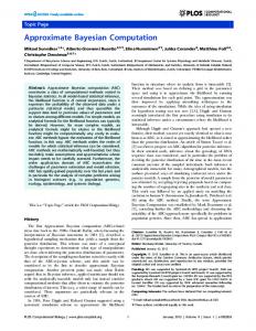
Figure 1: A simple Bayesian network
controversial, although it is adopted by major forensic laboratories, such as the Forensic Science Service of England and Wales [9]. Obviously, the approach is very useful when substantial data sets enable the analyst to calculate accurate estimates. This is the case in evaluating DNA evidence, for example [40]. Nevertheless, the approach can also be successfully applied to cases where the analyst has to rely on subjective probabilities, by performing a detailed sensitivity analysis [2] or by incorporating uncertainty concerning the probability estimates within the Bayesian model [21]. The likelihood ratio method is crucially dependent upon a means to compute the probabilities P (e | pprosecution ) and P (e | pdefense ). As shown in [2, 10], Bayesian Networks (BN) are a particularly useful technique in this context. A BN is a directed acyclic graph (DAG) whose nodes correspond to random variables and whose arcs describe how the variables are dependent upon one another. Each variable can be assigned a value, such as ”true” or ”false”, and each assignment of a value to a variable describes a particular situation of the real world (e.g. ”Jones has an alibi” is ”true”). The arcs have directions associated with them. Consider two nodes, A and B say, with a directed arc pointing from A to B. Node A is said to be the parent of B and B is said to be the child of A. Moreover, an arc from a node labelled H pointing towards a node labelled e indicates that e is dependent on H. The graph is acyclic in that it is not permitted to follow directed arcs and return to the starting position. Thus, a BN is a type of graphical model that captures probabilistic knowledge. The actual probabilistic knowledge is specified by probability distributions: a prior probability distribution P (xi ) : Dxi 7→ [0, 1] for each root node xi in the DAG and a conditional probability distribution P (xi | xj , . . . , xk ) : Dxi × Dxj × . . . × Dxk 7→ [0, 1] for each node xi that has a set of (immediate) parent nodes {xj , . . . , xk } (where Dx , the domain of variable x, denotes the set of all values that can be assigned to x). Figure 1 illustrates these concepts by a sample BN that describes how the assumed event of a perpetrator killing a victim (x1 ) is related to the possibility of discovering traces of blood on the victim matching the perpetrator’s blood (x5 ). The probabilistic knowledge represented by this BN is specified by probability distributions. There are two prior probability distributions P (x1 ) is read as the probability that the perpetrator has killed the victim and P (x4 ) read as the probability that the victim has the background they have, e.g. if a victim is a 20-year-old female student at a red-brick university, then P (x4 ) is the probability that a victim of rape is a 20-year-old female student at a red-brick university (in the absence of other information). This probability is a subjective one. There are three conditional probabilities P (x2 |x1 ), P (x3 |x2 , x1 ) and P (x5 |x4 , x3 ) where the probabilities of the various possible combinations of outcomes are represented in tables. Table 1 shows such an example.
4
P (x2 |x1 )
x1 : perpetrator killed victim
x2 : perpetrator had violent contact
True
False
True
0.9
0.3
False
0.1
0.7
with the victim
Table 1: Example conditional probability table
Given the figures of Table 1, the subjective probability that the perpetrator had violent contact with victim (x2 : true) given that the perpetrator killed the victim (x1 : true) is 0.9. BNs facilitate the computation of joint and conditional probabilities. This can be illustrated by calculating P (x5 : true | x1 : false). By definition, P
v2 ∈Dx2
P (x5 : true | x1 : false) =
P
v3 ∈Dx3
P
v4 ∈Dx4
P (x1 : false, x2 : v2 , x3 : v3 , x4 : v4 , x5 : true) P (x1 : false)
Note that in general, this calculation requires a substantial number of joint probabilities P (x1 : false, x2 : v2 , x3 : v3 , x4 : v4 , x5 : true). However, with the BN of Figure 1 and the corresponding conditional probability tables, the computation can be reduced to P (x5 : true | x3 : v3 , x4 : v4 )× P (x5 : true | x1 : false) =
X
X
X
P (x3 : v3 | x2 : v2 , x1 : false)×
v2 ∈Dx2 v3 ∈Dx3 v4 ∈Dx4
P (x2 : v2 | x1 : false) X X = P (x2 : v2 | x1 : false) × P (x3 : v3 | x2 : v2 , x1 : false)× v2 ∈Dx2
X
v3 ∈Dx3
P (x5 : true | x3 : v3 , x4 : v4 )
v4 ∈Dx4
As such, a BN can be employed both as a means to describe probabilistic knowledge and to calculate probabilities more efficiently. This increase in efficiency of the computation arises because the BN indicates which variables or factors are conditionally independent of each other. Thus the amount of blood traces found on the victim which match the perpetrator (x5 ) is independent of whether the perpetrator has killed the victim or not (x1 ) if the amount of blood traces transferred from the perpetrator to the victim is known (i.e. conditional on the knowledge of the amount of blood traces transferred from the perpetrator to the victim), x3 . This conditional independence is indicated by the separation of the node for x1 from x5 by x3 .
5
HUMAN INVESTIGATORS Investigation
Evidence
Investigative Actions
Speculation
Plausible Scenarios
Analysis
Knowledge Base
Synthesis
Bayesian Scenario Space DECISION SUPPORT SYSTEM
Explanations
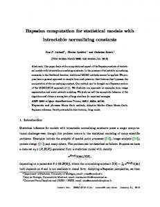
Figure 2: System Architecture
3
System Architecture
A drawback of the conventional Bayesian evidence evaluation approach is that it relies on BNs designed for evaluating specific types of evidence e with respect to specific hypotheses pprosecusion and pdefense . For example, the BN of Figure 1 is restricted to evaluate only blood transfer evidence with respect to a homicide hypothesis. As such, the approach requires careful consideration and specification of the hypotheses and the corresponding BNs. This limits the generality and reusability of the approach. The present work addresses this issue by (i) developing of a novel inference mechanism that can synthesise a BN which describes a range of plausible scenario and corresponding hypotheses, and (ii) employing Bayesian model based diagnostic techniques to evaluate evidence and to create evidence collection strategies with regard to synthesised scenarios or hypotheses.
The overall architecture of the resulting DSS is shown in Figure 2. Given a new or ongoing investigation in which an initial set of evidence has been collected by the investigators, the synthesis component will generate a large BN that contains a range of plausible scenarios, called the scenario space, by means of a knowledge base. The scenario space describes how plausible states and events, pieces of evidence, investigative actions and other properties of crime scenarios are causally related to one another. Note that this representation is substantially more efficient than one that considers a separate representation for each considered scenario because all the information that is shared by different scenarios is stored only once.
Once the scenario space has been constructed, the analysis component can evaluate it to provide useful information, such as (i) descriptions of scenarios that may have caused the available evidence, (ii) useful explanations for the human investigator (e.g what evidence should be expected if a certain scenario were true), and (iii) investigative actions that are likely to yield useful information. The proposed investigative actions can, in turn, be used to collect evidence or to speculate about the possible outcomes of the investigative action and determine future actions.
6
4
Knowledge Representation
4.1
Plausible situation
As this work concerns hypothetical crime scenarios, much reasoning focusses on plausible situations (i.e. a particular condition or status of the world) and events (i.e. a development that changes a situation). In what follows, the term “situation” will be employed to refer to both states and events that change states. Situations can be described at different levels of generality, depending on what is being modelled. In terms of relations between possible scenarios and a given specific case, the system supports the representation of situation instances at the information level, such as:
• “fibres were transferred from jane doe to joe bloggs” and • “many fibres were transferred from jane doe to joe bloggs”
Generally speaking, situation instances refer to information about specific entities, such as jane doe and joe bloggs. At the knowledge level, which relates to the understanding of the crime investigation domain, the system also supports representation of situation types, such as:
• “fibres were transferred from person P1 to person P2” and • “many fibres were transferred from person P1 to person P2”
Thus, situation types refer to certain general properties or relations of the classes of entities. As the examples illustrate, quantities and truth values are also an important feature of situations and events. In a manner similar to the distinction between types and instances, the system may sometimes be interested in situations and events that denote specific quantities and sometimes it may not. Situations and events that leave open specific quantities or truth values involved, such as
• “fibres were transferred from jane doe to joe bloggs” and • “fibres were transferred from person P1 to person P2”
are referred to as variables. Situations that do include specific quantities, such as
• “many fibres were transferred from jane doe to joe bloggs” and • “many fibres were transferred from person P1 to person P2”
7
are referred to as (variable) assignments, the variable being the ’quantity’ of the fibres transferred, where ’quantity’ can take, say, one of three values ’none’, ’few’, or ’many’.
To facilitate the integration of these features, variables are defined by tuples hp, Dp , vp , ⊕i. The variable defined by a tuple hp, Dp , vp , ⊕i is identified by a predicate p, has a domain Dp of values, including a default value vp ∈ Dp , that can be assigned to the variable, and is associated with a combination operator ⊕ : Dp × Dp 7→ Dp that describes how the effects of different influences acting upon the variable are combined. For reasons that will become clearer in the paper, the default value is set to be the neutral element of the combination operator in normal circumstances. For example, the tuple hprevious-hangings(johndoe), {never, veryfew, several}, never, maxi corresponds to a variable that describes the number of hangings johndoe survived before his death. Here, the max operator returns the greatest value of the domain, assuming that the ordering of values is as follows: never < veryfew < several.
Most variable assignments correspond to plausible states and events that are part of one or more possible scenarios. There are also special types of variable assignment that convey additional information that may aid in decision support. These concepts have been adapted from earlier work on abductive reasoning [46] and model based diagnosis [23]. In particular, some variable assignments correspond to evidence. These are pieces of known information that are considered to be observable consequences of a possible crime. Note that as evidence is defined as “information”, it does not equal the “exhibits” presented in court. Thus, for example, a suicide note is not considered to be a piece of evidence in itself, but the conclusion of a handwriting expert who has analysed the note is. Facts are pieces of known information that do not require an explanation. In practice, it is often convenient to accept some information at face value without elaborating possible justifications. For instance, when a person is charged with analysing the handwriting on a suicide note, the status of that person as a handwriting expert is normally deemed to be a fact. Hypotheses are possible answers to questions that must be addressed (by the investigators), reflecting certain important properties of a scenario. Typical examples of such hypotheses include the categorisation of a suspicious death into homicidal, suicidal, accidental or natural.
Also, assumptions are uncertain pieces of information that can be presumed to be true for the purpose of performing hypothetical reasoning. This work considers three types of assumption: (i) Investigative actions are assumptions that correspond to evidence collection efforts made by the investigators. For example, a variable assignment associated with the comparison of the handwriting on a suicide note and an identified sample of handwriting of the victim is an investigative action. Note that each investigative action a is associated with an exhaustive set Ea of mutually exclusive pieces of evidence that covers all possible outcomes of a. (ii) Default assumptions are assumptions that are presumed true unless they are contradicted. Such assumptions are typically employed to represent the conditions that an expert produces evaluations based upon sound methodology and understanding of his/her field. (iii) Conjectures correspond to uncertain states and events that need not be described as consequences of other states and events.
8
4.2
Knowledge Base
The objective of crime investigation is to determine (ideally beyond a reasonable doubt) the crucial features (such as the type of crime, the perpetrator(s), etc.) that have led to, or more precisely caused, the available evidence. Therefore, the domain knowledge that is relevant to crime investigation concerns the causal relations among the plausible situations.
4.2.1
Scenario fragments
These causal relations are stored in the knowledge base: The decision support system described in this paper employs a knowledge base consisting of generic causal relations, called scenario fragments, among situations. Each scenario fragment describes a phenomenon whereby a combination of situations leads to a new situation. In particular, each scenario fragment consists of (i) a rule representing which situation variable types are causally related, and (ii) a set of probability distributions that represent how the corresponding situation assignment types are related by the phenomenon in question. Formally, scenario fragments are represented by constructs of the form:
if {p1 , . . . , pk } assuming {pl , . . . , pm } then {pn } distribution pn { .. . v1 , . . . , vm ->vn1 : q1 , . . . , vnjn : qjn .. .
}
where {p1 , . . . , pk } is the set of antecedent predicates, {pl , . . . , pm } is the set of assumption predicates, pn is the consequent predicate, each vi , i ∈ {1, . . . , m}, is a value taken from the domain Dpi of the variable identified by pi and each qj is a real value in the range [0, 1]. The antecedent, assumption and consequent predicates identify situation variable types. The antecedents and assumptions of a rule refers to the situations that are required for the phenomenon described by the scenario fragment to take effect. The consequent describes the effect of the phenomenon. Note that the assumptions are situations that may be presumed to be present in a scenario because they refer to conjectures, default assumptions or investigative actions, and that the antecedents are themselves situations that must either be consequences of certain other scenario fragments or be factually true.
9
For example, the scenario fragment: if { anesthetic-substance(A) } assuming { is-addicted-to(P,A), has-recently-used(P,A) } then { carries-traces-in-blood-of(P,A) } distribution { true, true, true -> none:0, low:0.2, high: 0.8 true, false, true -> none:0.6, low:0.3, high:0.1 }
denotes that the likelihood of the conjectures ”P is addicted to an anesthetic substance A” and ”P has recently used anesthetic substance A” affects that of the situation that P’s blood carries traces of A. A scenario fragment, which has the variable types p1 , . . . , pm as its antecedents and assumptions and the variable type pn as its consequent, must also define a probability distribution over the possible assignments of pn , for each combination of assignments to p1 , . . . , pm . These distributions describe how the assignment of pn is affected by the phenomenon under different configurations of p1 , . . . , pm . Each line of the form
v1 , . . . , vm ->vn1 : q1 , . . . , vnjn : qjn
in the distribution component of a scenario fragment, defines such a probability distribution Dpn 7→ [0, 1] : f (vi ) = qi , for the combination of antecedent and assumption assignments p1 : v1 , . . . , pm : vm . In what follows, the probability (qi ) that the phenomenon described by scenario fragment S causes the consequent variable pn to take value vni given the assignments p1 : v1 , . . . , pm : vm will be denoted by:
S
P (p1 : v1 , . . . , pm : vm → pn : vni ) = qi
In the aforementioned example, let the domains of anesthetic-substance(A), is-addicted-to(P,A) and has-recently-used(P,A) be {false, true} and the domain of carries-traces-in-blood-of(P,A) be {none, low, high}. The scenario fragment is completed with specifications of probability distributions such as: true, true, true -> none:0, low:0.2, high: 0.8
which states that the phenomenon described by the scenario fragment has a probability of 0.8 to contribute a high number of traces of A to the blood of P, a probability of 0.2 to contribute a low number of traces of A to the blood of P and a probability of 0 to contribute no traces of A to the blood of P. Or, as this will be denoted in the remainder of this paper:
10
C
P (p1 : true, p2 : true, p3 : true → p4 : high) = 0.8 C
P (p1 : true, p2 : true, p3 : true → p4 : low) = 0.2 C
P (p1 : true, p2 : true, p3 : true → p4 : none) = 0 where C denotes the aforementioned example scenario fragment and p1 =anesthetic-substance(A), p2 =is-addicted-to(P,A), p3 =has-recently-used(P,A) and p4 =carries-traces-in-blood-of(P,A)
Note that it is not required that a probability distribution be defined for each combination of values assigned to the antecedent and assumption variables in a scenario fragment S. Instead, a probability distribution in which the default value of the consequent variable has a probability 1 is presumed. Here, the default probability distribution for those combinations of assignments p1 : v1 , . . . , pm : vm for which no probability distribution is defined, is
S
P (p1 : v1 , . . . , pm : vm → pn : v) =
1
v = vpn (i.e. the default value of pn )
0
otherwise
Let the default value of carries-traces-in-blood-of(P,A) be ’none’. Then, the aforementioned example scenario fragment also defines the following probability distribution implicitly: C
P (p1 : true, p2 : false, p3 : false → p4 : high) = 0 C
P (p1 : true, p2 : false, p3 : false → p4 : low) = 0 C
P (p1 : true, p2 : false, p3 : false → p4 : none) = 1
4.2.2
Inconsistencies
Some scenario fragments impose hard constraints on the possible scenarios. These scenario fragments are called inconsistencies. They contain a set of situation assignment types that are jointly impossible, and hence do not constitute any part of a sound scenario or a possible explanation. In the knowledge base, inconsistencies define inconsistent combinations of variable assignments. As such, an inconsistency denoting that p1 : v1 ∧ . . . ∧ pk : vk is inconsistent is represented as:
inconsistent {p1 : v1 , . . . , pk : vk }
11
For example, the following inconsistency states that a person can not be both killed by another person and by him/herself: inconsistent {commits-suicide-by(V,M):true, commits-homicide-by(P,V,M):true}
Inconsistencies are treated as a special type of scenario fragment of the form:
if {p1 , . . . , pk } then {nogood} distribution nogood { v1 , . . . , vk ->> : 1, . . . , ⊥ : 0}
where nogood refers to a special type of boolean variable, that remains hidden from the user and the knowledge engineer, and is known to be false. According to this definition, any situation where p1 : v1 , . . . , pk : vk requires nogood to be true. Consequently, the probability of p1 : v1 , . . . , pk : vk given that nogood is false, P (p1 : v1 , . . . , pk : vk | nogood : ⊥) = 0. And in this way, the inconsistency p1 : v1 , . . . , pk : vk is modelled as an impossibility. For example, the aforementioned inconsistency is treated as a scenario fragment of the form: if { commits-suicide-by(V,M), commits-homicide-by(P,V,M) } then { nogood } distribution nogood { true, true -> true:1, false:0 }
4.2.3
Prior distributions
In addition to scenario fragments, the knowledge base also contains prior distributions for assumed states and events. Prior distributions are represented by define prior p {v1 : q1 , . . . , vj : qj } where {v1 , . . . , vj } is the domain Dp of p and q1 , . . . , qj define a function fp : Dp 7→ [0, 1] : fp (vi ) = qi that is a probability distribution. For example, the definition define prior suicidal(V) {true:0.02, false:0.98}
12
specifies the prior probability distribution of a variable identified by suicidal(V) with the domain {true, false} and
fsuicidal(V) (true) = 0.02 fsuicidal(V) (false) = 0.98
Unless specified otherwise, a variable assignment represents an uncertain state or event. However, certain variable assignments can be associated with other types of information, such as hypotheses and evidence, in the knowledge base. Predicates identifying variables whose assignments correspond to hypotheses, facts, evidence, investigative actions and default assumptions are defined by purpose built constructs that associate certain types of predicate with one of these types of information (and corresponding to evidence sets, in the case of investigative actions). Conjectures contained in the knowledge base are identified in the assuming clause of the scenario fragments.
4.3
Presumptions
To enable their use in compositional modelling of BNs, it is presumed that the scenario fragments in a given knowledge base possess the following properties:
1. Any two probability distributions taken from two scenario fragments involving the same consequent variable are independent. Intuitively, this assumption indicates that, given the relevant antecedents and assumptions, the phenomena described by different scenario fragments that affect the same situation variable instance are independent from one another. 2. There are no cycles in the knowledge base. This means that there is no subset of scenario fragments in the knowledge base that allow a situation/event variable instance to be affected by itself. This assumption is required because BNs can not represent such information as they are inherently acyclic [45].
While presumption 1 is a strong assumption, and may hence reflect a significant limitation of the present work, it is required herein to efficiently compute the combined effect of a number of scenario fragments on a single variable (see 5.2). Future work will seek to relax this assumption in order to generalise further the application of the method proposed.
4.4
Example
Appendix A presents a sample knowledge base with which the remaining discussion will be illustrated. The knowledge contained within it relates to cases where a person died from hanging. To keep the example self-contained, the scope
13
johndoe asphyxiates self using rope r1 and johndoe planned to end self asphyxiation by cutting rope r1 with cutting instrument c1
cutting instrument c1 is near johndoe
person p1 overpowered johndoe using knife c1 and person p1 left knife c1 after overpowering johndoe
Figure 3: Partial scenario space of the knowledge base has been restricted and an imaginative reader may be able to produce plausible scenarios that are not covered by this knowledge base. It does, however, contain components of a broad range of scenarios, including those where the victim committed suicide, those where the victim was forcibly hanged by a murderer and those where the victim died accidentally whilst committing an act of autoerotic asphyxiation.
5
Scenario Space Synthesis
A scenario space is a grouping of all the scenarios that support the available evidence, and of the evidence and hypotheses that these scenarios entail. In a typical case, there may be many scenarios that explain the given evidence and most of these may only involve minor variations from the others in the same space. Therefore, it is not sensible to describe scenarios individually. Instead, the scenario space contains the situations that constitute scenarios and how they are causally related. Formally, a scenario space covers two sub-representations: the structural scenario space and the probabilistic scenario space:
• The structural scenario space denotes which combinations of situations affect other situations within the scenario space. Each situation in the structural scenario space is deemed to be either an assumption/fact or a consequent of other situations. For each sequence of situations, through the use of an assumption-based truth maintenance system [12], the structural scenario space maintains the smallest sets of other situations that can meaningfully explain it. Consider, for example, the partial structural scenario space depicted in Figure 3. This space identifies two plausible causes for ”cutting instrument c1 is near johndoe”: 1. A combination of events that may be part of an accidental auto-asphyxiation scenario: ”johndoe asphyxiates self using rope r1” and ”johndoe planned to end self asphyxiation by cutting rope r1 with cutting instrument c1”, and
14
2. A combination of events that may be part of a homicidal asphyxiation scenario: ”person p1 overpowered johndoe using knife c1” and ”person p1 left knife c1 after overpowering johndoe”. • The probabilistic scenario space denotes how likely a combination of situations affects other situations in the scenarios space. The probabilistic scenario space is a Bayesian network that refers to the same nodes as the structural scenario space. An example of a probabilistic scenario space is the Bayesian network depicted in Figure 1, with associated probability tables.
The structural and probabilistic versions of the scenario space reflect different types of information, providing complementary knowledge. While the structural scenario space does not provide a suitable means to test hypotheses or to evaluate evidence in an investigation, it enables the generation of explanatory scenarios, as illustrated in the example of Figure 3. Contrarily, while the probabilistic scenario space lacks the knowledge to produce minimally explanatory scenarios, it does, as shown in section 2, provide the necessary knowledge to test hypotheses and evaluate evidence. This section aims to demonstrate how both scenario spaces can be constructed from a given knowledge base.
5.1
Generating the structural scenario space
Informally, the scenario space structure contains:
(i) The hypothetical causes of the available evidence. As mentioned earlier, evidence has been defined as observable consequences of scenarios. Therefore, the probability of evidence is modelled causally. This is the approach taken by most of the existing abductive diagnostic techniques [23]. The decision support system seeks to identify combinations of these causes with each combination constituting a plausible crime scenario, and to help the human investigators differentiate between the likelihood of alternative scenarios. (ii) Additional potential evidence, yet undiscovered, that may exist as the consequences of the aforementioned causes. The decision support system discussed here seeks to identify which investigative activities might be the most effective at differentiating between the plausibility of alternative scenarios. This is in order to discover particular types of evidence. (iii) The plausible alternative hypothetical causes for the secondary evidence mentioned under (ii). This is required to correctly assess the likelihood of obtaining evidence through certain investigative activities. This information is employed to help determine which investigative activities are most effective. Note that these additional hypothetical causes are not part of the diagnostic problem in the way that the hypothetical causes mentioned under (i) are. It is not until they become plausible explanations of observed evidence that they have to be considered as such. For this reason, it is not necessary to consider additional evidence potentially resulting from the causes mentioned under (iii), until these causes may have explained observed evidence.
15
n1
N = {n1 , n2 , n3 , n4 , n5 , a1 , a2 , a3 }
∧
A = {a1 , a2 , a3 }
∧
J(n1 ) = {{n2 , n3 }, {n4 , n5 }}
n2
n3
n4
n5
∧
∧
∧
∧
a1
a2
J(n2 ) = {{a1 }} J(n3 ) = {{a1 , a2 }} J(n4 ) = {{a2 , a3 }} J(n5 ) = {{a3 }}
a3 Figure 4: Sample hypergraph hN, A, Ji
(iv) The combinations of causes mentioned in (i) and (iii) that are inconsistent. Certain combinations of situations and events can not be part of the same scenario because it is impossible that they are part of the same possible world. For example, when a person shoots someone across a long distance, transfer of blood splatter from the victim to the shooter as a result of the shot is impossible. Such inconsistent combinations of situations and events need to be identified, because they constrain which scenarios are plausible.
Formally, the structural scenario space is specified by a tuple hN, A, Ji where N denotes a set of nodes, A ⊂ N denotes a set of assumption nodes and J is a mapping that associates with each node n ∈ N a set J(n) of justifications. Each justification in J(n) is itself a set of nodes corresponding to a combination of variables influencing n. This is illustrated by the sample hypergraph shown in Figure 4 with the associated specification of hN, A, Ji. The structural scenario space is generated by means of two conventional inference techniques: (i) abduction of the plausible causes of known or hypothesised situations, and (ii) deduction of the plausible consequences of known or hypothesised situations. The abduction and deduction operations are applied to the emerging scenario space, by adapting the rules from the knowledge base to the specific circumstances described in the emerging scenario space:
• Abduction: given a piece of information that matches the consequent of a scenario fragment in the knowledge base, the abduction operation instantiates the information of the antecedents and assumptions of the rule, and adds them and the corresponding implication to the emerging scenario space. Consider, for example, the scenario fragment:
if { anesthetic-substance(A) } assuming { is-addicted-to(P,A), has-recently-used(P,A) } then { carries-traces-in-blood-of(P,A) } distribution { ... }
16
And, assume that the scenario space contains a variable instance that indicates that johndoe has traces of percocet in his blood: i.e. carries-traces-in-blood-of(johndoe, percocet) This situation matches the consequent of the aforementioned scenario fragment with a substitution σ = {A/percocet, P/johndoe}. By application of abduction to the aforementioned scenario fragment, the antecedent anestheticsubstance(percocet), and the assumptions is-addicted-to(johndoe, percocet) and has-recentlyused(johndoe, percocet) are generated, the implication anesthetic-substance(percocet)∧ is-addicted-to(johndoe, percocet)∧ has-recently-used(johndoe, percocet) → carries-traces-in-blood-of(johndoe, percocet)
is added to the emerging scenario space. Note that the antecedent of certain scenario fragments may contain variables that are not contained in the consequent. For example, the scenario fragment if { commits-homicide-by(P,V,M) } then { died-from(V,M) } distribution { ... }
states that if (a person) P successfully commits homicide of (person) V by means of (action) M, then it can be said that (person) V died from (action) M. Here, the antecedent contains variable P, which is not part of the consequent of the scenario fragment. Abduction of such rules requires that new instance names are created for those variables that the antecedent introduces. Following the Prolog convention, such instances will be given a name of the form n, where n is an automatically generated integer: e.g. 1. • Deduction: given a set of pieces of information that match the antecedents of a scenario fragment in the knowledge base, the deduction operation instantiates the information of the assumptions and consequent of the rule, and adds them and the corresponding implication to the emerging scenario space. Consider, for example, the following scenario fragment: if { investigator(I), has-symptom(L,S), petechiae(S) } assuming { correct-diagnosis(I,S) } then { has-petechiae(L) } distribution { ... }
17
And, assume that investigator watson makes an observation (of purple spots), herein identified as 1, on the eyes of johndoe and that that observation corresponds to petechiae: i.e. investigator(watson), has-symptom(eyes(johndoe),_1), petechiae(_1) } This situation matches the consequent of the aforementioned scenario fragment with a substitution σ = {I/watson, L/eyes(johndoe), S/ 1}. By application of deduction to the above scenario fragment, the assumption correctdiagnosis(watson, 1, is-addicted-to(johndoe, percocet) and the piece of evidence has-petechiae( eyes(johndoe)) are generated and the implication investigator(watson) ∧ has-symptom(eyes(johndoe), 1)∧ petechiae( 1) ∧ correct-diagnosis(watson, 1) → has-petechiae(eyes(johndoe))
is added to the emerging scenario space.
A formal specification of the procedure that generates structural scenario spaces is given by Algorithm 5.1. That is, CONSTRUCT S CENARIO S PACE S TRUCTURE(K, I, S, F )
synthesises a structural scenario space hN, A, Ji for a given set
of scenario fragments K, a set of established inconsistencies I, a set S of available evidence and a set F of known facts. Algorithm 5.1: CONSTRUCT S CENARIO S PACE S TRUCTURE(K, I, S, F ) hN, A, Ji ← INITIALISE S CENARIO S PACE(S, F ); ABDUCE C AUSES (hN, A, Ji, K); DEDUCE C ONSEQUENCES (hN, A, Ji, K); ABDUCE C AUSES (hN, A, Ji, K); DEDUCE C ONSEQUENCES (hN, A, Ji, I); SPURIOUS N ODE R EMOVAL (hN, A, Ji);
return (hN, A, Ji);
Algorithm 5.1 consists of 6 steps:
1. Initialisation: A new symbolic scenario space is first created containing only the known facts and pieces of evidence and no inferences between them. More precisely, Algorithm 5.1 first initialises the hypergraph with the procedure INITIALISE S CENARIO S PACE(S, F ), which is specified as Algorithm 5.2.
with the following justfications: J(n) =
{}
if n ∈ S
{{}}
if n ∈ F
18
This results in a hypergraph S ∪ F, F, Ji,
In other words, the pieces of evidence receive no justification yet and the facts are justified by the empty set because they are deemed true under all circumstances. Algorithm 5.2: INITIALISE S CENARIO S PACE(S, F ) N ← new set; A ← new set; J ← new table; for each p ∈ S, N ← N ∪ {p}; for each p ∈ F N ← N ∪ {p}; do A ← A ∪ {p}; return (hN, A, Ji); The procedure will be illustrated using the knowledge base of Appendix A . For simplicity, a situation with only a single piece of evidence will be assumed: the hanging body of man named johndoe. In this case, the initialisation phase produces a partial structural scenario space with only one node labelled evidence(hanging(body(johndoe))). 2. Abduction of plausible causes from collected evidence: The abduction operation explained above is applied with all the scenario fragments in the knowledge base whose consequent matches a situation variable instance in the emerging scenario space. In this way, causal chains of situations that constitute plausible explanations for the available evidence are constructed. Algorithm 5.3: ABDUCE C AUSES(hN, A, Ji, K) for each substitution(σ), hif Pantecent assuming Passumptions then {pc }distribution Di ∈ K, σpn ∈ N E ← new set; for each pi ∈ Pantecedent ∪ Passumptions if σpi 6∈ N p ← instantiate(σpi ); N ← N ∪ {p}; do do then if pi ∈ Passumptions then A ← A ∪ {p}; E ← E ∪ {p}; else E ← E ∪ {σp }; i J(σp ) ← J(σp ) ∪ {E}; c c
19
suicidal(johndoe)
chooses−suicide−method
commits−suicide−by(
died−from(johndoe,
evidence(hanging(
(johndoe,hanging)
johndoe,hanging)
hanging)
body(johndoe)))
is−killer(_1,johndoe)
commits−homicide−by( _1,johndoe,hanging)
chooses−homicide− method(_1,hanging) autoerotic−asphyxiation− habit(johndoe)
accidental−autoerotic− hanging(johndoe)
fatal−autoerotic− asphyxiation−method( johndoe)
Figure 5: Hypergraph generated after applying Algorithm 5.3 in Step 2. Note: the shaded boxes represent new nodes added in this step of the procedure.
Formally, Algorithm 5.3 generates these explanations for the available evidence, by instantiating scenario fragments in K. For each scenario fragment, whose consequent variable matches a node in N , the predicates describing the antecedent and assumption variables are instantiated and added to N if these instances do not already exist. A set E containing the antecedent and assumption instances is added to the set of justifications associated with the consequent. Note that the matching of those predicates specifying variables in N with the predicates in the scenario fragment is accomplished with a set of substitutions σ.
Figure 5 depicts a sample partial scenario space that would emerge after this step if the knowledge base of Appendix A and the single piece of evidence introduced in Step 1 are employed.
3. Deduction of plausible consequences from plausible causes: The deduction operation explained above is applied with all the scenario fragments in the knowledge base whose antecedents match a set of situation variable instances in the emerging scenario space. In so doing, causal chains containing the consequences of those situations that are plausible causes of the available evidence are generated. The objective of this step in the overall procedure is to infer the evidence that has not yet been identified, but may be produced by plausible scenarios that explain the available evidence. As discussed below, it is important to identify these pieces of evidence because this information helps the system in supporting the investigator to determine which of the scenarios that explain the available evidence may be more plausible.
20
Algorithm 5.4: DEDUCE C ONSEQUENCES(hN, A, JiK) for each substitution(σ), hif Pantecent assuming Passumptions then {pc }distribution Di ∈ K, {σpi | pi ∈ Pantecedent } ⊂ N if σpc 6∈ N p0 ← instantiate(σpc ); N ← N ∪ {p0 }; E ← new set; for each pi ∈ Pantecedent do E ← E ∪ {σpi }; for each pi ∈ Passumptions do if σpi 6∈ N then p ← instantiate(σpi ); N ← N ∪ {p}; do then A ← A ∪ {p}; E ← E ∪ {p}; else E ← E ∪ {σpi }; J(p0 ) ← J(p0 ) ∪ {E};
Algorithm 5.4 generates all possible consequences of the explanations created previously. For each scenario fragment, whose antecedent variables match instances in N , the predicates describing the assumption and consequent variables are instantiated and added to N if they do not already exist. As in the previous phase, a set E containing the antecedent and assumption instances is added to the set of justifications associated with the consequent. Continuing with the ongoing example, Figure 6 depicts a sample partial scenario space that would emerge after this step. 4. Abduction of plausible causes from uncollected evidence: When assessing the value of searching for additional evidence through further investigative actions, it is important that the entire range of possible causes of such evidence is considered, not just the causes that reside within the crime scenarios. For example, when searching for gun powder residue on the hands of a suspect, the possible role of this suspect in the crime under investigation is not the only relevant plausible explanation for a potential discovery of gun powder residue. The background of the suspect may constitute an alternative explanation when, for instance, the suspect is an amateur hunter. Therefore, Step 2 of the procedure is repeated for the pieces of uncollected, but potentially available evidence, which have been deduced in Step 3. The partial scenario space that results from this step of the structural scenario space synthesis algorithm is shown in
21
suicidal!death(johndoe)
examine( eyes(johndoe))
suicidal(johndoe)
attempted!suicide( johndoe)
cause!of!death(johndoe, asphyxiation)
petechiae(eyes(johndoe))
chooses!suicide!method (johndoe,hanging)
commits!suicide!by( johndoe,hanging)
died!from(johndoe, hanging)
evidence(hanging( body(johndoe)))
drugged!self(johndoe)
toxscreen(johndoe)
overpowers(_1,johndoe)
was!anaesthetised( johndoe)
is!killer(_1,johndoe)
commits!homicide!by( _1,johndoe,hanging)
evidence(anaesthetics( johndoe))
evidence(self!harm( johndoe))
chooses!homicide! method(_1,hanging)
head!injury(johndoe)
was!forced(johndoe)
homicidal!death(johndoe)
autoerotic!asphyxiation! habit(johndoe)
evidence(petechiae( eyes(johndoe)))
evaluate!knot(johndoe)
knot!analysis(johndoe)
accidental!autoerotic! hanging(johndoe)
previous! hangings(johndoe)
fatal!autoerotic! asphyxiation!method( johndoe)
evidence(head!injury( johndoe)) evidence(defensive! wounds(johndoe))
examine( body(johndoe))
evidence(previous! hangings(home(johndoe)))
search(home(johndoe), previous!hangings) choice!of!autoerotic! hanging!method(johndoe)
accidental!death(johndoe)
leaves!cutting!instrument! near(_1,johndoe)
cutting!instrument! near(johndoe)
evidence(cutting! instrument!near(johndoe))
search(near(johndoe), cutting!instrument)
Figure 6: Hypergraph generated after applying Algorithm 5.4 in Step 3. Note: the shaded boxes represent new nodes added in this step of the procedure.
22
suicidal−death(johndoe)
examine( eyes(johndoe)) attempted−suicide(
cause−of−death(johndoe,
johndoe)
asphyxiation)
chooses−suicide−method
commits−suicide−by(
died−from(johndoe,
evidence(hanging(
(johndoe,hanging)
johndoe,hanging)
hanging)
body(johndoe)))
drugged−self(johndoe)
toxscreen(johndoe)
suicidal(johndoe)
is−killer(_1,johndoe)
commits−homicide−by( _1,johndoe,hanging)
overpowers(_1,johndoe)
petechiae(eyes(johndoe))
evidence(petechiae( eyes(johndoe)))
evidence(anaesthetics( johndoe))
was−anaesthetised( johndoe)
chooses−homicide−
evidence(self−harm( johndoe))
method(_1,hanging)
other−source−of− anaesthetics(johndoe)
head−injury(johndoe)
evidence(head−injury( johndoe))
other−source−of− head−injury(johndoe)
was−forced(johndoe)
evidence(defensive− wounds(johndoe))
homicidal−death(johndoe)
autoerotic−asphyxiation− habit(johndoe)
examine( body(johndoe))
evaluate−knot(johndoe)
knot−analysis(johndoe)
accidental−autoerotic−
previous−
evidence(previous−
hanging(johndoe)
hangings(johndoe)
hangings(home(johndoe)))
fatal−autoerotic− asphyxiation−method(
search(home(johndoe),
johndoe)
previous−hangings) choice−of−autoerotic− hanging−method(johndoe)
accidental−death(johndoe)
leaves−cutting−instrument−
cutting−instrument−
evidence(cutting−
near(_1,johndoe)
near(johndoe)
instrument−near(johndoe))
cutting−instrument−was−at−
search(near(johndoe),
crime−scene(johndoe)
cutting−instrument)
Figure 7: Hypergraph generated after applying Algorithm 5.3 in Step 4. Note: the shaded boxes represent new nodes added in this step of the procedure.
23
suicidal!death(johndoe)
examine( eyes(johndoe))
suicidal(johndoe)
chooses!suicide!method (johndoe,hanging)
is!killer(_1,johndoe)
attempted!suicide(
cause!of!death(johndoe,
johndoe)
asphyxiation)
commits!suicide!by( johndoe,hanging)
died!from(johndoe, hanging)
evidence(hanging( body(johndoe)))
drugged!self(johndoe)
toxscreen(johndoe)
overpowers(_1,johndoe)
was!anaesthetised( johndoe)
other!source!of! anaesthetics(johndoe)
head!injury(johndoe)
other!source!of! head!injury(johndoe)
was!forced(johndoe)
homicidal!death(johndoe)
examine( body(johndoe))
commits!homicide!by( _1,johndoe,hanging)
chooses!homicide! method(_1,hanging)
NOGOOD
autoerotic!asphyxiation! habit(johndoe)
evaluate!knot(johndoe)
knot!analysis(johndoe)
accidental!autoerotic! hanging(johndoe)
previous! hangings(johndoe)
fatal!autoerotic! asphyxiation!method( johndoe)
petechiae(eyes(johndoe))
evidence(petechiae( eyes(johndoe)))
evidence(anaesthetics( johndoe))
evidence(self!harm( johndoe)) evidence(head!injury( johndoe)) evidence(defensive! wounds(johndoe))
evidence(previous! hangings(home(johndoe)))
search(home(johndoe), previous!hangings) choice!of!autoerotic! hanging!method(johndoe)
accidental!death(johndoe)
leaves!cutting!instrument! near(_1,johndoe)
cutting!instrument! near(johndoe)
cutting!instrument!was!at!
search(near(johndoe),
crime!scene(johndoe)
cutting!instrument)
evidence(cutting! instrument!near(johndoe))
Figure 8: Hypergraph generated after deducing inconsistences in Step 5
Figure 7. 5. Deduction of inconsistencies: Once a symbolic scenario space has been constructed that contains the available evidence (Step 1), the possible causes of the available evidence (Step 2), the possible but uncollected evidence that may be generated by these possible causes (Step 3) and the possible causes of the uncollected evidence (Step 4), any given constraints under which situations that may be part of the same scenario are added to the emerging symbolic scenario space. This involves applying a deduction operation for each inconsistency whose situation variables match a set of situation variables in the emerging symbolic scenario space. The partial scenario space that results from this step of the structural scenario space synthesis algorithm is shown in Figure 8. 6. Spurious explanation removal: The structural scenario space generated by the above procedure enables the decision support system to trace back the conjectures and facts that could originally have caused the available evidence. Because such causal chains may have to be established by multiple abduction operations applying different scenario fragments, it is possible that the resulting structural scenario space contains situations that are not a consequence of any situation and that are not assumptions or facts. As explained in section 4, assumptions and facts are the only types of information that require no further explanation. Their role as so-called root nodes in the scenario space is
24
extended in the probabilistic scenario space as they represent the only information which is associated with a prior distribution. Therefore, such nodes constitute spurious explanations, and they are to be removed from the emerging scenario space. The following procedure recursively removes from a given hypergraph hN, A, Ji all root nodes that do not correspond to a fact/assumption and the justifications in which these nodes occur. The procedure terminates when each root node in hN, A, Ji corresponds to either a fact or an assumption. In effect, this procedure deletes all spurious nodes and justifications from the hypergraph. Algorithm 5.5: SPURIOUS N ODE R EMOVAL(hN, A, Ji) � for each n ∈ N, (@substitution(σ), J(n) = ∅, n 6∈ A N ← N \{n}; do for each n0 , E ∈ J(n0 ), (n ∈ E) ∧ (n0 ∈ N ) do J(n0 ) ← J(n0 )\E;
As the hypergraph of Figure 8 does not contain any spurious nodes, consider the following scenario fragment as a means of illustration: if {victim(Victim)} assuming { suspect(Perpetrator), fight(Perpetrator,Victim), fight(Victim,Perpetrator)} then {transfer(fibres,Victim,Perpetrator)} if {victim(Victim)} assuming { suspect(Perpetrator), fight(Perpetrator,Victim), fight(Victim,Perpetrator)} then {transfer(fibres,Perpetrator,Victim)} Given evidence transfer(fibres, 1, johndoe), the symbolic scenario space generator will create the following information: victim(johndoe), suspect(johndoe), victim( 1), suspect( 1), fight( 1, johndoe) and fight(johndoe, 1). Here, victim(johndoe) : > is a fact. Furthermore, suspect(johndoe) and suspect( 1) correspond to assumption nodes, where suspect(johndoe) : > should be rendered impossible by means of an inconsistency. victim( 1) is neither fact nor assumption, and it is not further justified. Therefore, the node containing victim( 1) is spurious and must be removed.
5.2
Generating the probabilistic scenario space
As explained above, the probabilistic scenario space is a Bayesian network (BN) that represents the extent to which the situations in the structural scenario space affect one another. Such a scenario space is created by following the procedure
25
below:
• For each situation variable instance in the structural scenario space, create a corresponding node; • For each implication . . . ∧ a ∧ . . . → c, where a and c refer to situation variable instances, create an arc a → c; • For each assumption or fact in the structural scenario space, which (as defined above) is always represented by a parent node and not by a child node, obtain a prior probability distribution, which must either be predefined in the knowledge base or be specified by the user; and • For each node that does not correspond to an assumption or fact, calculate a conditional probability distribution table based on the probability distributions associated with each scenario fragment.
The first three steps of this procedure are straightforward and are formally specified as follows: Algorithm 5.6: CREATE DAG(hN, A, Ji) G ← new DAG; for each n ∈ N add(G, n); � S return (G); do for each n0 ∈ E E∈J(n) do add(G, arc(n0 , n));
The generation of the conditional probability tables is somewhat more complex. Therefore, the remainder of this subsection is dedicated to this topic. Let {p1 , . . . , ps } be the set of parents of pn in the probabilistic scenario space, pc : c be an assignment of pc , and A be a set of assignments {p1 : v1 , . . . , ps : vs }, where each vi ∈ Dpi . The conditional probability of the situation pc : c given A is determined by those scenario fragments that determine how the situations p1 : v1 , . . . , ps : vs affect pc . Let SF1 , . . . , SFk be such scenario fragments and pc : c1 , . . . , pc : ck be their respective outcomes. pc is assigned c whenever the combined effect of the scenario fragments c1 ⊕ . . . ⊕ ck = c, with regard to a certain predefined interpretation of the combination operator ⊕. From this, the conditional probability P (pc : c | A) is given by:
" P (pn : c | A) = P
!# _
^
c1 ⊕...⊕ck =c
i=1,...,k
SFi
A → pn : ci
�
(2)
Thus, computing P (pn : c | A) involves calculating the likelihood of a combination of events described by a disjunctive normal form (DNF) expression (i.e. an expression of the form (x11 and . . . and x1m1 ) or . . . or (xn1 and . . . and xnmn )).
26
Because the occurrence of the different combinations of outcomes c1 , . . . , ck of scenario fragments SF1 , . . . , SFk involves mutually exclusive events, the calculation can be resolved by adding the probabilities of the conjuncts in (2):
! P (pn : c | A) =
X
P
c1 ⊕...⊕ck =c
SFi
^
A → pn : ci
�
(3)
i=1,...,k
From presumption 1 (as noted in 4.3), the outcomes of different scenario fragments (of the same consequent), with regard to a given set of assignments of the antecedent and assumption variables, correspond to independent events. Therefore, the probability of the conjunctions in (3) is equal to the product of the probabilities of their conjuncts, thereby
! P (pn : c | A) =
X
Y
c1 ⊕...⊕ck =c
i=1,...,k
SFi
P A → pn : ci
�
(4)
Consider the following two scenario fragments, which form part of the probabilistic scenario space that corresponds to the structural space of Figure 8:
if { autoerotic-asphyxiation-habit(V) } then { previous-hangings(V) } distribution previous-hangings(V) { true -> never:0.1, veryfew:0.4, several:0.5 } if { attempted-suicide(V) } then { previous-hangings(V) } distribution previous-hangings(V) { true -> never:0.7, veryfew:0.29, several:0.01 }
where autoerotic-asphyxiation-habit(V) and attempted-suicide(V) correspond to boolean variables, and previous-hangings(V) to a variable taking values from the (totally ordered) domain {never, veryfew, several}, with never →1 p3 : never) = 0.10 SF
P (p1 : > →1 p3 : veryfew) = 0.40 SF
P (p1 : > →1 p3 : several) = 0.50 SF
P (p2 : > →2 p3 : never) = 0.70 SF
P (p2 : > →2 p3 : veryfew) = 0.29 SF
P (p2 : > →2 p3 : several) = 0.01
Then, the probabilities of assignments to previous-hangings(V), given that autoerotic-asphyxiation-habit(V) and attempted-suicide(V) are assigned true (or the probabilities of assignments to p3 given p1 : > and p2 : >), can be computed as follows. According to (4), all combinations of the outcomes c1 and c2 of scenario fragments SF1 and SF2 , with c1 , c2 ∈ {never, veryfew, several}, such that max(c1 , c2 ) = veryfew, must be considered. There are three such combinations: {c1 : veryfew, c2 : veryfew}, {c1 : never, c2 : veryfew} and {c1 : veryfew, c2 : never}. Hence, P (p3 : veryfew|p1 : >, p2 : >) can be computed by
P (p3 :veryfew|p1 : >, p2 : >) SF
SF
=P (p1 : > →1 p3 : veryfew) × P (p2 : > →2 p3 : veryfew)+ SF
SF
P (p1 : > →1 p3 : never) × P (p2 : > →2 p3 : veryfew)+ SF
SF
P (p1 : > →1 p3 : veryfew) × P (p2 : > →2 p3 : never) =0.4 × 0.29 + 0.1 × 0.29 + 0.4 × 0.7 = 0.425
Similarly, it can be shown that P (p3 : never|p1 : >, p2 : >) = 0.070 P (p3 : several|p1 : >, p2 : >) = 0.505
The complete scenario space for the ongoing example is a Bayesian network containing 43 variables, 28 conditional probability tables and 15 prior probability distributions. Clearly, any representation of the full specification of this network, and the computations required for belief propagation by means of this network, would significantly add to the size of this paper while contributing little new knowledge. Thus, only a part of this BN is shown in Figure 9 for illustration, which relates to the corresponding part of the scenario space of Figure 5.
28
n1 suicidal(johndoe)
n7
n10
n11
commits−suicide−by(
died−from(johndoe,
evidence(hanging(
johndoe,hanging)
v1
true false
P (n1 : v1 )
0.02 0.98
true
(johndoe,hanging)
v2
true false
P (n2 : v2 )
0.1
false
v2 true
1
0
false
0
1
true
0
1
false
0
1
v7
v8 true
true false
true
n3
n8
is−killer(_1,johndoe)
commits−homicide−by(
false false
_1,johndoe,hanging)
true false
P (n3 : v3 )
0.01 0.99
n4 chooses−homicide− method(_1,hanging)
v4
true false
P (n4 : v4 )
0.05 0.95
true
false
true
1
false
0
1
true
0
1
false
0
1
n9
true false
P (n5 : v5 )
0.01 0.99
v6 P (n6 : v6 )
true
1
0
0
false
0
1
true
1
0
false
1
0
true
1
0
false
1
0
true
1
0
false
0
1
v9
true
asphyxiation−method( johndoe)
0
1
hanging(johndoe)
n6 fatal−autoerotic−
1
P (n9 : v9 |n5 : v5 , n6 : v6 ) v5
v6
true false
true
1
0
false
0
1
true 0.05 0.95 false
false
0
1
true false 0.0250.975
Figure 9: Sample partial Bayesian network
29
true false
true
0
accidental−autoerotic−
v10
false
true false
n5
v5
v11
true false
v8 v4
autoerotic−asphyxiation− habit(johndoe)
v9
P (n8 : v8 |n3 : v3 , n4 : v4 ) v3
P (n11 : v11 |n10 : v10 )
v10
true false
0.9
v3
body(johndoe)))
P (n10 : v10 |n7 : v7 , n8 : v8 , n9 : v9 )
v7 v1
n2 chooses−suicide−method
hanging)
P (n7 : v7 |n1 : v1 , n2 : v2 )
6
Scenario Space Analysis
Once constructed, the probabilistic scenario space can be analysed in conjunction with the structural one to compute effective evidence collection strategies. The concepts of evidence, hypotheses, assumptions and facts are still employed in the probabilistic scenario space, but they now refer to variable assignments instead of predicates. For implementational simplicity, hypotheses and investigative actions are assumed to be represented by (truth) assignments to boolean variables (although this can be extended). The work will be illustrated by means of probabilities derived from a BN which has been generated by means of the techniques of section 5 using the knowledge base of Appendix A (and which is a Bayesian representation of the symbolic scenario space given in Figure 8).
6.1
Hypothesis sets and query types
The approach shown here aims to interpret the investigatory worth of different scenarios in relation to a set H of hypotheses. This set must be exhaustive and the hypotheses within it mutually exclusive. The set H is exhaustive if one of the hypotheses in the set is guaranteed to be true. This ensures that the approach will evaluate the scenario space entirely. The hypotheses in a set are mutually exclusive if no pair of hypotheses taken from the set can be true simultaneously. This simplifies the interpretation of entropy values because it ensures that a situation of total certainty corresponds to an entropy value of 0. These conditions may seem to be rather strong in general, but they are not strong for the present work. This is because the exhaustivity is only subject to the demand for the generated space to be fully examined in the evaluation, while different scenarios naturally satisfy the requirement that only one underlying scenario be true at any one time. An example of a hypothesis set that meets these criteria is:
H = {death of johndoe was homicide : >, death of johndoe was suicide : >, death of johndoe was accidental : >, death of johndoe was natural : >}
In this work, hypothesis sets are predefined in the knowledge base along with a precompiled taxonomy of query types. Query types represent important questions that the investigators need to address, such as the type of cause of death of a victim in a suspicious death case, or the killer of a victim in a homicide case. Query types are identified with a predicate describing it and they may be associated with a set of predicates identifying the hypothesis variables. For example, the following two query type definitions
30
define query type { unifiable = type-of-death(P), hypotheses = {homicidal-death(P),suicidal-death(P), accidental-death(P),natural-death(P)}} define query type { unifiable = killer-of(P), hypotheses = {killed(Q,P)}}
are respectively associated with the following hypothesis sets:
H1 = {homicidal-death(johndoe) : >, suicidal-death(johndoe) : >, accidental-death(johndoe) : >, natural-death(johndoe) : >} H2 = {killed(mr-hyde,mary-kelly) : >, killed(jack-the-ripper,mary-kelly) : >, killed( 1,mary-kelly) : >, killed(none,mary-kelly) : >}
It is the responsibility of the knowledge engineer to ensure that the hypothesis sets generated in this way meet the exhaustiveness and mutual exclusivity criteria. These criteria can be satisfied for any given set P = {p1 , . . . , pn } of predicates identifying hypothesis variables. Exhaustiveness can be assured by extending P with an additional predicate pn+1 and adding a probabilistic scenario fragment that enforces pn+1 : > with likelihood 1 if p1 : ⊥, . . . , pn : ⊥, and pn+1 : ⊥ with likelihood 1 otherwise:
if {p1 , . . . , pn } then {pn+1 } distribution pn+1 {⊥, . . . , ⊥->> : 1, ⊥ : 0}
The mutual exclusivity criterion can be easily achieved by adding inconsistencies for each pair of hypotheses:
inconsistent {pi : >, pj : >}
31
6.2
Entropy
As indicated previously, the work here employs an information theory based approach, which is widely used in areas such as machine learning [39] and model based diagnosis [23]. Information theory utilises the concept of entropy, which is a measurement of doubt over a range of choices. Applied to the present problem, the entropy over an exhaustive set of mutually exclusive hypotheses H = {h1 , . . . , hm } is given by:
�(H) = −
X
P (h) log P (h)
h∈H
where the log base is 2, and the values P (h) can be computed by conventional BN inference techniques. Intuitively, entropy can be interpreted as a quantification of a lack of information. Under the exhaustiveness and mutual exclusivity conditions, it can be shown that �(H) reaches its highest value (which corresponds to a total lack of information) when P (h1 ) = . . . = P (hm ) =
1 m
and �(H) reaches 0, its lowest value (which corresponds to a totally certain situation) when
all P (hi ) = 0, i = 1, . . . , j − 1, j + 1, . . . , m and P (hj ) = 1, j ∈ {1, . . . , m}. In crime investigation, additional information is created through evidence collection. Thus, the entropy metric for the purpose of generating evidence collection strategies is the entropy over a set of hypotheses H, given a set E = {e1 : v1 , . . . , en : vn } of pieces of evidence:
�(H | E) = −
X
P (h | E) log P (h | E)
(5)
h∈H
where the values P (h | E) can, again, be computed through BN inference. This expression may be considered as a measure of the lack of information H given E. For the example problem from the sample scenario space, the following probabilities can be computed, with E1 containing evidence(hanging(body(johndoe))) : > and nogood : ⊥:
P (homicidal-death(johndoe) | E1 ) = 0.22 P (suicidal-death(johndoe) | E1 ) = 0.33 P (accidental-death(johndoe) | E1 ) = 0.45
Thus, as an instance,
P (H1 | E1 ) = −(0.22 log 0.22 + 0.33 log 0.33 + 0.45 log 0.45) = 1.53
32
A useful evidence collection strategy involves selecting investigative actions from a given set A according to the following criterion:
min Exp(�(H | E), a) a∈A
(6)
Note that the entropy values calculated by (5) are affected by the prior distributions assigned to the assumptions, as described in section 4. Within the context of evidence evaluation (which often applies the likelihood ratio based approach [1]), this is a controversial issue as decisions regarding the likelihood of priors, such as the probability that a victim had autoerotic hanging habits, are a matter for the courts to decide. In the context of an investigation, however, these prior distributions may provide helpful information often ignored by less experienced investigators. For example, the probability of suicides or autoerotic deaths are often underestimated. As such, the strategy dictated by (6) offers a useful means to decide on what evidence to collect next. Nevertheless, the minimal entropy decision rule does not yield information that should be used for evidence evaluation in court.
6.3
Minimal entropy-based evidence collection
Let a denote an investigative action and Ea be a set of the variable assignments corresponding to the possible outcomes of a (i.e. the pieces of evidence that may result from the investigative action). The expected posterior entropy (EPE) after performing a can then be computed by calculating the average of the posterior entropies with regard to the different possible outcomes e ∈ Ea , weighted by the likelihood of obtaining each outcome e (given the available evidence):
Exp(�(H | E), a) =
X
P (e | a : >, E)�(H | E ∪ {a : >, e})
(7)
e∈Ea
The ongoing example contains an investigative action a =test-toxicology(johndoe): >, representing a toxicology test of johndoe searching for traces of anaesthetics and a corresponding set of outcomes Ea = {toxscreen(johndoe) : >, toxscreen (johndoe) : ⊥}, respectively denoting a positive toxscreen and a negative one. Let E2 be a set containing hanging-dead-body (johndoe) : >, text-toxicology(johndoe) : > and nogood : ⊥. Then, through exploiting the Bayesian scenario space the following can be computed:
33
P (toxscreen(johndoe) : > | E2 ) = 0.17 P (toxscreen(johndoe) : ⊥ | E2 ) = 0.83 P (homicidal-death(johndoe) | E2 ∪ {toxscreen(johndoe) : >}) = 0.40 P (suicidal-death(johndoe) | E2 ∪ {toxscreen(johndoe) : >}) = 0.49 P (accidental-death(johndoe) | E2 ∪ {toxscreen(johndoe) : >}) = 0.11 P (homicidal-death(johndoe) | E2 ∪ {toxscreen(johndoe) : ⊥}) = 0.19 P (suicidal-death(johndoe) | E2 ∪ {toxscreen(johndoe) : ⊥}) = 0.44 P (accidental-death(johndoe) | E2 ∪ {toxscreen(johndoe) : ⊥}) = 0.38
Intuitively, these probabilities can be explained as follows. In a homicide, anaesthetics may have been used by the murderer to gain control over johndoe, and in a suicide case, johndoe may have used anaesthetics during the suicide process. In the accidental (autoerotic) death case, there is no particular reason for johndoe to be anaesthetised. Therefore, the discovery of traces of anaesthetics in johndoe’s body supports both the homicidal and suicidal death hypotheses whilst disaffirming the accidental death hypothesis. By means of these probabilities, the EPEs can be computed as the following instance:
Exp(�(H | E1 ), a) =0.17 × −(0.40 log 0.40 + 0.49 log 0.49 + 0.11 log 0.11)+ 0.83 × −(0.19 log 0.19 + 0.44 log 0.44 + 0.38 log 0.38) =0.17 × 1.38 + 0.83 × 1.51 = 1.49
The investigative action that is expected to provide the most information is the one that minimises the corresponding EPE. For example, Table 2 shows a number of possible investigative actions that can be undertaken (in column 1) and the corresponding EPEs in the sample probabilistic scenario space (in column 2) computed on the assumption that the aforementioned toxicology screen yielded a positive result. The most effective investigative actions in this case are therefore established to be a knot analysis and an examination of the body. This result can be intuitively explained by the fact that these investigative actions are effective at differentiating between homicidal and suicidal deaths, which have both been the most likely hypotheses if anaesthetics are discovered in the body.
6.4
Extensions
While the approach presented above is itself a useful alternative to the likelihood ratio approach, several further improvements of this proposed technique are proposed. As these extensions are not difficult to conceive, detailed examples are
34
omitted below.
6.4.1
Local optima and action sequences
Although the minimum EPE evidence collection technique guarantees to return an effective investigative action, it does not ensure globally optimal evidence collection. This limitation is inherent to any such one-step lookahead optimisation approach. The likelihood of obtaining low quality locally optimal evidence collection strategies can be reduced by considering the EPEs after performing a sequence of actions a1 , . . . , av (of course, with incurred overheads over computation):
Exp(�(H | E), a1 , . . . , av ) X X P (e1 , . . . , ev | a1 : >, . . . , av : >, E) = ... e1 ∈Ea1
(8)
ev ∈Eav
�(H | e1 , a1 : >, . . . , ev , av : >, E)
In order to determine Exp(�(H | E), a1 , . . . , av ), equation (8) can be simplified as follows:
Exp(�(H | E), a1 , . . . , av ) X X P (e1 , . . . , ev , a1 : >, . . . , av : >, E) = ... a1 : >, . . . , av : >, E e1 ∈Ea1
ev ∈Eav
�(H | E ∪ {e1 , a1 : >, . . . , ev , av : >}) =
X
...
e1 ∈Ea1
X ev ∈Eav
v Y P (ei , a1 : >, . . . , av : >, E) � a1 : >, . . . , av : >, E i=1
(9)
�(H | E ∪ {e1 , a1 : >, . . . , ev , av : >}) =
X e1 ∈Ea1
...
X
v Y
� P (ei | a1 : >, . . . , av : >, E)
ev ∈Eav i=1
�(H | E ∪ {e1 , a1 : >, . . . , ev , av : >})
6.4.2
Multiple evidence sets
Certain investigative actions may be associated with multiple sets of evidence. For example, a careful examination of the body of a man found hanging may yield various observations such as petechiae on the eyes, defensive wounds on the hands and lower arms, and various types of discolouration of the body. The consequences of some types of investigative
35
action, e.g. the examination of a dead body, are better modelled by multiple evidence sets since the outcomes may occur in any combination of such pieces of evidence. The above approach can be readily extended to account for this by computing the EPEs after performing action a with associated evidence sets Ea,1 , . . . , Ea,w :
Exp(�(H | E), a) X X P (e1 , . . . , ew | a : >, E) ... = ew ∈Ea,w
e1 ∈Ea,1
�(H | e1 , . . . , ew , a : >, E) =
X
...
e1 ∈Ea,1
X
w Y
P (ei | a : >, E)
(10)
�
ew ∈Ea,w i=1
�(H | E ∪ {e1 , . . . , ew , a : >})
6.4.3
Multiple hypothesis sets
Finally, it may also be useful to consider multiple hypothesis sets instead of just one. This enables the decision support system to propose evidence collection strategies that are effective at answering multiple queries. To consider multiple hypothesis sets H1 , . . . , Ht by measuring entropy over these sets, given a set of pieces of evidence E, the following is required:
�(H1 , . . . , Ht | E) X X =− ... P (h1 , . . . , ht | E) log P (h1 , . . . , ht | E) h1 ∈H1
=−
X h1 ∈H1
6.5
(11)
ht ∈Ht
...
t X Y
t Y � � P (hi | E) log P (hi | E)
ht ∈Ht i=1
i=1
User interface
While a detailed discussion of the user interface developed for the present system is beyond the scope of this paper, it is important to point out that a mere representation of the outcomes of the decision rules is inadequate for realising the objectives of the system. Investigators may have a number of considerations that are beyond the scope of the current implementation. These may include perishability of evidence, legal restrictions, limitations on resources and overall workload. Therefore, the implemented system has been devised to list alternative evidence collection strategies in increasing order of EPEs.
36
Investigative action
EPE
NEER
REER
Knot analysis
0.98
26%
29%
Examine body
1.12
17%
19%
Search for cutting instrument
1.19
13%
14%
Search for signs of previous hangings
1.36
1.3%
1.5%
Check eyes for petechiae
1.38
0%
0%
Table 2: Evaluation of investigative actions The benefits of each strategy is indicated by either the normalised expected entropy reduction (NEER) or the relative expected entropy reduction (REER). The NEER represents the reduction in EPE due to performing an investigative action a (i.e. �(H | E) − Exp(�(H | E), a)) as a proportion of the maximal entropy under total lack of information. As such, it provides a means of assessing case progress:
N EER(H | E, a) =
�(H | E) − Exp(�(H | E), a) �(H)
(12)
The REER represents EPE reduction as a proportion of the entropy under the current set of available evidence; it focuses on the relative benefits of each alternative investigative action possible:
REER(H | E, a) =
�(H | E) − Exp(�(H | E), a) �(H | E)
(13)
These calculations are illustrated in Table 2 for the running example. As mentioned previously, this table presents the evaluation of a number of investigative actions after traces of anaesthetics have been discovered in johndoe’s body. The second column of this table displays the EPEs for investigative action while the third and fourth columns show the corresponding NEER and REER values respectively.
7 7.1
Discussions Related work
Evidential reasoning is an important, current topic in Artificial Intelligence and Law. A broad range of systems have been developed for this purpose. The system presented here is distinct from the existing literature in that it addresses a different but nonetheless significant problem in evidential reasoning: hypothesis synthesis and their analysis with a view to devising evidence collection strategies.
37
Argumentation systems [8, 38, 47, 55, 58] and probabilistic expert systems [2, 9, 40] are primarily intended to support evidential reasoning in courts. Most argumentation systems represent plausible causes as consequences of obtained evidence, in order to contrast alternate lines of reasoning [49]. One notable exception is AVER, which combines the aforementioned explanatory (observation-to-cause) inferences with causal (cause-to-effect) inferences [3]. AVER, however, aims to model investigators’ narratives; it is not designed to support the calculation of effective evidence collection strategies. Probabilistic expert systems aim to calculate the extent to which a single piece of evidence supports one scenario rather than competing scenarios, with a view to justify the testimony of forensic experts in court [9]. Thus, these types of system are designed to be employed after the evidence collection effort that the DSS described here supports. Data mining systems for intelligence databases [6, 30, 42, 60] and other types of data analysis tool [16, 24, 25, 48, 54] seek to identify possible crimes. While such tools determine whether there is evidence of elements of a certain crime scenario, they are not intended to reconstruct plausible alternatives of crime scenarios. In other words, these types of system support analysis of plausible crimes rather than plausible scenarios of a single crime. As such, they are designed to be employed before an individual case is examined in detail.
7.2
Scaling up applications
The DSS described herein incorporates the methodologies for scientific inquiry in crime investigation, following the best practice proposed by forensic scientists [9, 29]. A prototypical system has been developed, and it was evaluated in collaboration with forensic scientists at the Forensic Laboratory of a UK Police Force, with regard to a number of solicited knowledge bases. A small-scale example of such a knowledge base is shown in the appendix. This has demonstrated the DSS’s ability to construct and simultaneously analyse a broad variety of plausible crime scenarios from compact knowledge bases. As such, the system is potentially able to support the construction and refinement of plausible scenarios during the early investigation of serious crimes. This is a novel development and distinguishes the DSS described herein from the other DSSs built in the domain of crime investigation. The present work contains two key features that facilitate scaled up applications. Firstly, the compositional modelling approach allows causal knowledge concerning specific aspects of hypothetical situations and events, or specific types of evidence to be defined from first principles. First principles can be considered in isolation from the extraneous context, such as unrelated or partially related conjecture and evidence or any investigative procedure, in which it is used. Such knowledge is less complex and more reusable compared to experienced whole cases. More specifically, individual serious crime cases reoccur relatively infrequently compared to the constituent hypothetical events and evidence. As such, the use of a knowledge base relying on first principles makes the approach more robust. Similar observations have been made in the domain of physical systems diagnosis [7]. Secondly, the maximum entropy reduction approach, when applied to the model space, is capable of considering a large number of plausible scenarios and relating them to available evidence and investigative activities. It has the ability to
38
identify the potentially most productive evidence collection strategies. This is beneficial as simultaneous analysis of multiple scenarios, in order to guide an ongoing investigation, is an area in which both human investigators and conventional decision support systems lack. Despite these advantages, difficulties in deploying such a system remain. These issues and ways in which these difficulties may be resolved are discussed in the remainder of this section.
7.3
First principles and the ceteris paribus assumption
As indicated previously, the approach presented herein builds on model based reasoning techniques that have been applied successfully in the physical domain. Of course, there are crucial differences between the natural science, which studies physical systems, and forensic science, which studies crime scenarios. The most important of these is that the behaviour of physical systems can be described by first principles that can be applied ceteris paribus (i.e. under the assumption of all other things being equal). While there are certain first principles in the forensic science domain, the ceteris paribus clause generally does not hold. A key reason for this is that crime scenes are not pristine, uncontaminated places [41]. Consequently, there are many factors that may affect the way in which combinations of causes influence (observable) consequences. For example, the amount of blood splatter transferred from the victim to the perpetrator due to an assault with a blunt instrument is proportional to the extent and duration of the assault. There are many factors that may make subsequent discovery of blood splatter on the perpetrator matching the victim more or less likely (e.g. the propensity of the victim to bleed as a consequence of injury, the existence of blood from sources other than the victim on the perpetrator’s clothes, etc.). Therefore, the presumption of independence of any two probability distributions taken from two scenario fragments involving the same consequent variable is difficult to uphold.
7.4
Subjective probability
Obviously, first principles in the forensic science domain are often a matter of approximation. Many factors need to be considered in determining the effect of an influence (e.g. the number of fibres transferred between two people involved in a physical altercation). It is extremely difficult, if not impossible, to model such factors precisely in practice. The use of probabilities may allow for uncertainty which is associated with the effects resulting from unknown or unconsidered factors to be expressed. However, probability distributions over scenario fragments usually stem from subjective assessments by experts rather than from experimental estimation. Therefore, the use of numeric probabilities conveys an inappropriate degree of precision [22]. This issue can be examined in more detail by considering a thought experiment as proposed in [56]. In such an experiment, a game is played between two experts using the following procedure. First, one expert offers a price q for a promise to pay 1 currency unit if a proposition of interest, denoted by p : v here, turns out to be correct. Next, the other expert decides whether the first one may buy or sell such a promise. Finally, the actual proposition is revealed. Thus, q is a price at which the first expert is neutral between buying or selling a promise to pay 1 currency unit if p : v is correct. The outcome
39
of the game is that, according to the first expert, P (p : v) = q. As such, this thought experiment provides a way to attach semantics to the subjective probabilities that are suggested by experts. In practice, however, experts are reluctant to commit to such numerical values. This implies that there is no a single obvious price at which experts are neutral between buying and selling a promise of the aforementioned kind. There exists a range of extensions on classical Pascalian probability theory that facilitate capturing subjective probabilities by means of this thought experiment. These approaches are based on the use of intervals of probabilities, rather than the conventional point probabilities. An interval offers a richer representation to capture an expert’s belief. In terms of the thought experiment of [56], the lower boundary of a probability interval, associated with a particular proposition and suggested by an expert, corresponds to the highest price at which the expert is willing to buy a promise to pay 1 currency unit if the proposition is revealed to be true. Similarly, the upper boundary of the probability interval corresponds to the lowest price at which the expert is willing to sell a promise to pay 1 currency unit if the proposition is revealed to be true. Approaches that use probability intervals include qualitative probability networks and qualitative certainty networks [4, 15, 50], and also the order-of-magnitude based extensions thereof [43, 44]. Recent work has shown that QPNs with orderof-magnitude calculus can be adapted to express second-order influences (i.e. influences that affect the effect of other influences) [31]. Such second-order influences include, for example, inhibitors that reduce the effect of another influence, and amplifiers that increase the effect of another influence. Thus, they provide a mechanism to represent, in the form of scenario fragments, considerations that may sway an influence’s outcome from its ceteris paribus effect. Furthermore, the influences in QPNs are easily compoundable into more complex models without the need for unrealistic assumptions, and they are intrinsically approximate in nature. As such, this line of research has great potential to address the aforementioned concerns. More sophisticated variations on the interval based approach employ sets of intervals. These include second-order probability theory [11, 20, 57] and linguistic probability theory [22]. Such approaches relate probability intervals to another metric concerning each individual interval. This may be an expression of confidence in the interval, as in second-order probability theory, or a degree of belonging described by means of fuzzy membership values, as in linguistic probability theory.
7.5
Domain knowledge acquisition
In this work, the DSS’ knowledge base is presumed to contain generic causal relations. These relations formalise how crime scenario events and situations have observable consequences that may be collected and analysed to form evidence. Analogously, typical forensic science textbooks describe types of evidence, the methodology for their identification, collection and preservation, and plausible causes [28, 59]. Because serious crimes are relatively rare, the sets of evidence involved with such offences tend to be rare also or even unique. Individual features of crime scenarios, and individual types of event and evidence occur significantly more frequently than any specific scenario they may be part of. Variations
40
on plausible case scenarios may share substantial subsets of situations, events and evidence in common. Therefore, the underlying approach proposed here employs a knowledge representation formalism that models causal relations between typical events and aspects of situations, rather than scenarios as a whole (which conventional case-based approaches tend to make use of). This enables the resulting DSS to be based on a relatively small knowledge base to produce significantly large sets of scenarios. Nevertheless, scaling up the DSS for generating plausible crime scenarios is constrained by the knowledge acquisition bottleneck, i.e. the difficulty of eliciting and modelling relevant domain knowledge. This has important implications. The completeness of the knowledge base has a significant impact upon the accuracy of the decision support advice that is to be produced. Missing variables and influences may be part of plausible scenarios that explain all the evidence whilst proving a substantially different scenario. Also, missing variables/influences may affect certain conditional probability distributions, though this is a limitation not specific to the present approach but shared by all techniques for knowledge model creation. The use of first principles, as inspired by model based reasoning, alleviates this concern to a certain extent [23]. However, issues such as the need to consider situations that undermine the ceteris paribus assumption make it very difficult to fully exploit the benefits that model-based reasoning offers in the physical systems domain. Therefore, it remains the case that the development of knowledge bases for the system discussed herein requires a substantial amount of effort. The requirement to build a reasonably complete knowledge base prior to the deployment of the DSS is likely to be the greatest obstacle to said deployment. Model based reasoning with first principles forms the core of this work. Some first principles can be derived from the literature on evidential reasoning. For example, a methodology has been developed to assess witness testimony by separating plausible discrepancies between testimony and hypothetical events in terms of witness veracity, witness objectivity and observational sensitivity of the witness [51]. A Bayesian network has been devised to model two-way trace evidence transfer that is broadly applicable to a wide range of evidence types (not only those that are traditionally considered trace evidence but also, for instance, digital forensics evidence) [2]. Yet, generally speaking, the elicitation of first principles to developed a knowledge base for the system described here is more difficult because it involves the challenging hypothesis synthesis that makes serious crime investigation difficult. Expert practitioners need to be involved with the development of a knowledge base. Increasingly, expert forensic scientists have been developing Bayesian networks for evidential reasoning in particular domains. For example, most recently, Bayesian networks have been designed to analyse the evidence with respect to hypothetical scenarios which may be encountered in cases of suspected piracy via BitTorrent [37]. Such developments provide formal representations of knowledge that can be ported to a knowledge base required to support the present work, with relative ease. Research on other types of diagram representing evidential reasoning about serious crimes, such as Wigmore charts, also constitutes a potentially valuable source to acquire knowledge from [26]. Given the practical and case-specific nature of forensic science and crime investigation [41], plausible crime scenarios and,
41
sometimes, the corresponding first principles are only considered during the investigation of a particular case. Tools to represent such scenarios and alternatives between them have recently been developed [3], however. A potentially fruitful avenue of future research would therefore be the development of methods to extract reuseable scenario fragments from plausible crime scenarios as they emerge during the course of an investigation. Such techniques would help to automate significant portions of the process of knowledge acquisition, effectively providing a knowledge management approach for forensic laboratories and police forces. A number of research challenges need to be addressed to support this development, of course. Firstly, representational consistency in the description of hypothetical scenarios and the emerging knowledge base is required. This suggests that a formal ontology would need to be introduced [19]. Secondly, an appropriate mechanism for generalisation of approximate and imprecise first principles is needed. The field of machine learning provides a wealth of methods to potentially accomplish this. However, machine learning approaches typically perform generalisation through speculation that is driven by a method-specific inductive bias [39]. Therefore, and thirdly, a novel technique is necessary to identify emerging inconsistencies in the knowledge base and to correct them during the learning process.
7.6
Usability
The development of a suitable interface to the DSS presented herein is essential to its successful application. As part of the evaluation of the prototypical system that has been implemented (and which is described in [52]), the software has been demonstrated to practitioners, including forensic scientists, police investigators and lawyers. This subsection summarises key findings regarding usability issues [13] that have arisen from this informal, but user-driven part of the evaluation. The DSS presented here is capable of producing information that police investigators and forensic scientists find particularly useful in a number of aspects. These include: (a) hypothetical explanations of available evidence, (b) additional justifications that discriminate between likely hypotheses (as opposed to evidence that merely confirms preferred hypotheses), (c) representations of plausible scenarios, and (d) rankings of further investigating actions in terms of their potential relative effectiveness. The system is considered to be very helpful, especially for novice investigators. In particular, educational software has been proposed on several occasions, as a potential alternative application (for investigator training). The information or advice that the present DSS may provide, as discussed in section 6, is not suitable for use in court. The entropy measurements defined therein are based on the posterior probabilities of hypotheses. They vary (ultimately) from the values assigned to the prior probabilities. Prior probabilities of hypotheses can provide a helpful start point in an investigation in the absence of a null hypothesis. It may be based on neutrality between alternative hypotheses (i.e. P (h1 ) = P (h2 ) = . . . = P (hm )) or reflect expert knowledge (e.g. relative homicide and suicide rates appropriate to the victim’s profile). In a court setting, such prior probabilities represent a bias, and prior probabilities are eliminated from the analysis in this setting by employing the likelihood ratio outlined in section 2. However, the Bayesian networks generated by the DSS presented may be employed for this purpose.
42
Forensic scientists commenting on the usefulness of this approach have pointed out that the causal representation of hypothetical scenarios or larger proportions of the scenario space may be of particular significance. The representation scheme was considered to match well with their scientific approach to an investigation. The prototype software is capable of displaying subsets of a scenario space such as the one shown in Figure 8. The terms in the nodes of the diagram are converted into descriptive text and they can be colour coded to indicate the role (e.g. conjecture, hypothesis, evidence) of each node. One possible view is a single plausible scenario that explains a given set of available evidence or a certain hypothesis. Knowledge produced by the system can thus be presented in a way that is manageable by the user. Another important feature of the causal diagrams is that the nodes can also be colour coded to indicate the relative likelihood of the constituent terms of the diagram, either given a particular scenario (for likelihood ratio calculations) or given a set of observations. Police investigators generally regard these diagrams as useful but incomplete given the nature of their work. Police officers are particularly constrained by various procedures, policies, perishability of evidence, time and other important considerations such as victim support. For example, each police organisation will have forms, procedures and information systems devised to record and maintain collected evidence, and these are updated as new technologies are introduced (e.g. geotagging). It is crucial that an extended, and hence deployable, version of the prototypical system can be integrated with such existing systems. More generally speaking, the design of an interface that incorporates such information as well for police users remains an important practical issue. Finally, lawyers tend to employ the information produced by the DSS as part of their arguments. Most of their reasoning typically derives from the evidence. While most practicing lawyers do this with narratives, without the benefit of diagrams, forward-looking legal professionals do employ one of a variety of argument diagramming techniques. Virtually all of these diagramming techniques use evidence rather than hypothetical causes as their origin and reason in a effect-to-cause rather than a cause-to-effect direction [49]. They also employ a richer ontological framework to categorise the role of evidence and premises in an argument (such as so-called primary and ancillary evidence and premises) as well as the way one line of reasoning relates to another. However, the development of such argument structures crucially depends upon the generation of plausible hypotheses, as well as an assessment of the strength of support a given piece of evidence provides for one premise as opposed to another [51]. As such, a valuable line of inquiry is the exploration of the relationships and synergies between Bayesian networks (and scenario spaces in general) on the one hand and argument diagrams on the other hand. Recently, work has been developed to explore such relationships and synergies between Hugin style object-oriented Bayesian networks and Wigmore charts [26].
8
Conclusion
This paper has introduced a novel compositional modelling approach to generating Bayesian networks (BN), called scenario spaces, which describe a range of plausible crime scenarios that are sufficient to explain a given set of available
43
evidence. A scenario space contains a network of plausible states and events, factually and potentially available evidence, investigating actions, and hypotheses describing important properties of some of the plausible scenarios. It models how these elements of scenarios are causally related and what constraints are imposed over them. Such a space provides an efficient means of storing a wide range of scenarios, because the elements that different scenarios have in common need only be recorded once. The paper has also extended Bayesian model-based diagnosis techniques to identifying the most likely hypotheses and to refining diagnostic classifications by effective evidence collection strategies. A set of maximum expected entropy reduction techniques have been devised that can identify the investigative actions that are expected to yield the most conclusive evidence. Therefore, the work presented here enables the development of a novel type of decision support system for aiding less experienced crime investigators in constructing effective evidence collection strategies. This has been demonstrated in the paper by means of a realistic application example. While the proposed approach offers useful functionalities for developing DSSs and shows great potential, a number of further improvements are possible. As the probability distributions captured within the scenario fragments may refer to subjective assessments by experts, of the likely outcomes, which are actually described in vague terms, the use of numeric probabilities conveys an inappropriate degree of precision. Section 7.4 explored a range of extensions to Pascalian probability calculus that can be employed to facilitate elicitation of subjective probabilities. It has indicated why intervalbased approaches and their extensions may make it easier for experts to express their beliefs. However, in order to validate this theoretical argument, the use of such probability calculi has to be evaluated either through experiments purposefully designed or by deploying the system for a specific setting and assessing its use. This will constitute a significant piece of empirical research. Another piece of interesting further research concerns the relaxation of two important assumptions made within this work: (1) probability distributions, which govern the outcomes of different causal influences that may affect the same variable, are independent, and (2) the effects of all causal influences affecting the same variable are combinable using a single type of composition operator. Relaxing these assumptions is essential to allow the approach to be scaled up. It has been demonstrated that the use of qualitative probability calculi and extensions thereof will allow such assumptions to be relaxed through the use of second-order influences, which may affect the existence, strength and direction of other influences [31]. Further development of this work is necessary however, as well as empirical work to evaluate the feasibility of eliciting such knowledge in practice for more complex problems. As discussed above, the key challenge in future work lies with the acquisition of scenario fragments in general, and the probability distributions therein, in particular. The paper has identified a number of important issues and proposed potentially useful research directions in an effort to address this challenge. However, as the present work has only been evaluated by a relatively small-scale example, further investigation is needed to arrive at a more complete understanding of the nature of the knowledge acquisition bottleneck(s) in this particular problem domain. To accomplish this, a case-study involving a larger scale domain is required, which remains as active research.
44
Acknowledgements This work has been supported in part by the Nuffield Foundation Grant NAL/32370 and UK EPSRC grant GR/S63267. The authors are very grateful to Colin Aitken, Mark Lee, Tom Nelson and Burkhard Schafer for helpful discussions and assistance, whilst taking full responsibility for the views expressed here. The authors are also grateful to the anonymous referees for their constructive comments which have helped improve this paper considerably.
A
Sample Knowledge Base
assuming {suicidal(V)} then {attempted-suicide(V)} distribution attempted-suicide(V) { true -> true:0.8, false 0.2}
if {other-cause-of-head-injury(V)} then {head-injury(V)} distribution head-injury(V) { true -> true:0.3, false:0.7}
if {attempted-suicide(V)} then {previous-hangings(V)} distribution previous-hangings(V) { true -> never:0.7, veryfew:0.29, several:0.01}
if {overpowers(P,V)} then {was-forced(V)} distribution was-forced(V) { true -> true:0.334, false:0.666}
assuming {suicidal(V), chooses-suicide-method(V,M)} then {commits-suicide-by(V,M)} distribution commits-suicide-by(V,M) { true, true -> true:1, false:0}
assuming {autoerotic-asphyxiation-habit(V), fatal-autoerotic-asphyxiation-method(V,hanging)} then {accidental-autoerotic-hanging(V) } distribution accidental-autoerotic-hanging(V) { true, true -> true:1, false:0 false, true -> true:0.05, false:0.95}
if {commits-suicide-by(V,hanging)} then {drugged-self(V)} distribution drugged-self(V) { true -> true:0.15, false:0.85}
if {accidental-autoerotic-hanging(V)} then {died-from(V,hanging)} distribution died-from(V,hanging) { true -> true:1, false:0}
if {other-cause-of-anaesthetics(V)} then {was-anaesthetised(V)} distribution was-anaesthetised(V) { true -> true:1, false:0}
if {accidental-autoerotic-hanging(V)} then {accidental-death(V)} distribution accidental-death(V) { true -> true:1, false:0}
if {drugged-self(V)} then {was-anaesthetised(V)} distribution was-anaesthetised(V) { true -> true:1, false:0}
if {commits-homicide-by(P,V,M), accidental-autoerotic-hanging(V)} assuming {choice-of-autoerotic-hanging-method(V), evaluate-knot(V)} then {knot-analysis(V)} distribution knot-analysis(V) { true, false, detachable, true -> not-self-made:1, detachable:0, cutable:0, undetermined:0 true, false, cutable, true -> not-self-made:1, detachable:0, cutable:0, undetermined:0 false, true, detachable, true -> not-self-made:0, detachable:1, cutable:0, undetermined:0 false, true, cutable, true -> not-self-made:0, detachable:0, cutable:1, undetermined:0}
if {commits-suicide-by(V,M)} then {died-from(V,M)} distribution died-from(V,M) { true -> true:1, false:0} if {commits-suicide-by(V,M)} then {suicidal-death(V)} distribution suicidal-death(V) { true -> true:1, false:0} assuming {is-killer(P,V), chooses-homicide-method(P,M)} then {commits-homicide-by(P,V,M)} distribution commits-homicide-by(P,V,M) { true, true -> true:1, false:0}
assuming {choice-of-autoerotic-hanging-method(V)} then {cutting-instrument-near(V)} distribution cutting-instrument-near(V) { cutting-instrument -> true:1, false:0}
if {commits-homicide-by(P,V,M)} then {died-from(V,M)} distribution died-from(V,M) { true -> true:1, false:0}
assuming {cutting-instrument-was-at-crime-scene(V)} then {cutting-instrument-near(V)} distribution cutting-instrument-near(V) { true -> true:1, false:0}
if {commits-homicide-by(P,V,M)} then {homicidal-death(V)} distribution homicidal-death(V) { true -> true:1, false:0}
if {commits-suicide-by(P,V,hanging)} assuming {leaves-cutting-instrument-near(P,V)} then {cutting-instrument-near(V)} distribution cutting-instrument-near(V) { true -> true:1, false:0}
if {commits-homicide-by(P,V,hanging)} then {overpowers(P,V)} distribution overpowers(P,V) { true -> true:0.95, false:0.05}
if {autoerotic-asphyxiation-habit(V)} then {previous-hangings(V)} distribution previous-hangings(V) { true -> never:0.1, veryfew:0.4, several:0.5}
if {overpowers(P,V)} then {was-anaesthetised(V)} distribution was-anaesthetised(V) { true -> true:0.3, false:0.7}
if {died-from(V,hanging)} then {cause-of-death(V,asphyxiation)} distribution cause-of-death(V,asphyxiation) { true -> true:1, false:0}
if {overpowers(P,V)} then {head-injury(V)} distribution head-injury(V) { true -> true:0.3, false:0.7}
if {died-from(V,hanging)}
45
then {evidence(hanging(body(V)))} distribution evidence(hanging(body(V))) { true -> true:1, false:0}
several, true -> true:0.95, false:0.05} if {cutting-instrument-near(V)} assuming {search(near(V),cutting-instrument)} then {evidence(cutting-instrument-near(V))} distribution evidence(cutting-instrument-near(V)) { true, true -> true:0.9, false:0.1}
if {cause-of-death(V,asphyxiation)} then {petechiae(eyes(V))} distribution petechiae(eyes(V)) { true -> true:0.99, false:0.01} if {petechiae(eyes(V))} assuming {examination(eyes(V))} then {evidence(petechiae(V))} distribution evidence(petechiae(V)) { true, true -> true:0.99, false:0.01}
inconsistent {commits-suicide-by(V,M):true, commits-homicide-by(P,V,M):true} inconsistent {commits-suicide-by(V,M):true, accidental-autoerotic-hanging(V):true}
if {was-anaesthetised(V)} assuming {toxscreen(V)} then {evidence(anaesthetics(V))} distribution evidence(anaesthetics(V)) { true, true -> true:0.95, false:0.05 false, true -> true:0.01, false:0.99}
inconsistent {commits-homicide-by(P,V,hanging):true, accidental-autoerotic-hanging(V):true} inconsistent {leaves-cutting-instrument-near(P,V):true, accidental-autoerotic-hanging(V):true}
if {head-injury(V)} assuming {examine(body(V))} then {evidence(head-injury(V))} distribution evidence(head-injury(V)) { true, true -> true:1, false:0 false, true -> true:0.1, false:0.9}
define prior suicidal(V) {true:0.02, false:0.98} define prior chooses-suicide-method(V,hanging) { true:0.1, false:0.9} define prior is-killer(P,V) { true:0.01, false:0.99}
if {was-forced(V)} assuming {examine(body(V))} then {evidence(defensive-wounds(V))} distribution evidence(defensive-wounds(V)) { true, true -> true:1, false:0 false, true -> true:0.1, false:0.9}
define prior chooses-homicide-method(P,hanging) { true:0.05, false:0.95} define prior autoerotic-asphyxiation-habit(V) { true:0.025, false:0.975}
if {attempted-suicide(V)} assuming {examine(body(V))} then {evidence(self-harm(V))} distribution evidence(self-harm(V)) { true, true -> true:0.7, false:0.3 false, true -> true:0.1, false:0.9}
define prior fatal-autoerotic-hanging(V) { true:0.01, false:0.99} define prior other-cause-of-anaesthetics(V) { true:0.05, false:0.95}
if {previous-hangings(V)} assuming {search(home(V),previous-hangings)} then {evidence(previous-hangings(V))} distribution evidence(previous-hangings(V)) { veryfew, true -> true:0.2, false:0.8
define prior other-cause-of-head-injury(V) { true:0.05, false:0.95} define prior leaves-cutting-instrument-near(P,V) { true:0.5, false:0.5}
References [1] C. Aitken and F. Taroni. Statistics and the evaluation of evidence. Wiley, 2004. [2] C. Aitken, F. Taroni, and P. Garbolino. A graphical model for the evaluation of cross-transfer evidence in DNA profiles. Theoretical Population Biology, 63(3):179–190, 2003. [3] F. Bex, S. van den Braak, H. van Oostendorp, H. Prakken, B. Verheij, and G. Vreeswijk. Sense-making software for crime investigation: how to combine stories and arguments? Law, Probability and Risk, 6:145–168, 2007. [4] A. Biedermann and F. Taroni. Bayesian networks and probabilistic reasoning about scientific evidence when there is a lack of data. Forensic Science International, 157(2–3):163–167, 2006. [5] M. Bromby, M. MacMillan, and P. McKellar. A CommonKADS representation for a knowledge based system to evaluate eyewitness identification. International Review of Law Computers and Technology, 17(1):99–108, 2003. [6] H. Chen, J Schroeder, R.V. Hauck, L. Ridgeway, H. Atabakhsh, H. Gupta, C. Boarman, K. Rasmussen, and A.W. Clements. COPLINK Connect: Information and knowledge management for law enforcement. Decision Support Systems: Special Issue on Digital Government, 34(3):271–285, 2002.
46
[7] J. Chen and R. Patton. Robust model-based fault diagnosis for dynamic systems. Kluwer Academic Publishers, 1999. [8] J. Conklin and M. Begeman. gIBIS: a hypertext tool for exploratory policy discussion. ACM Transactions on Office Information Systems, 4(6):303–331, 1988. [9] R. Cook, I. Evett, G. Jackson, P. Jones, and J. Lambert. A model for case assessment and interpretation. Science and Justice, 38:151–156, 1998. [10] R. Cook, I. Evett, G. Jackson, P. Jones, and J. Lambert. Case pre-assessment and review in a two-way transfer case. Science and Justice, 39:103–111, 1999. [11] G. de Cooman. Precision - imprecision equivalence in a broad class of imprecise hierarchical uncertainty models. Journal of Statistical Planning and Inference, 105(1):175–198, 2002. [12] J. de Kleer. An assumption-based TMS. Artificial Intelligence, 28:127–162, 1986. [13] A. Dix, J. Finlay, G. Abowd, and R. Beale. Human-Computer Interaction. Prentice Hall, third edition edition, 2004. [14] D. Dixon. Police investigative procedures. In C. Walker and K. Starmer, editors, Miscarriage of Justice. A Review of Justice in Error, pages 65–82, 1999. [15] M. Druzdzel and M. Henrion. Efficient reasoning in qualitative probabilistic networks. In Proceedings of the 11th Conference on Artificial Intelligence, pages 548–553, 1993. [16] D. Dzemydiene and V. Rudzkiene. Multiple regression analysis in crime pattern warehouse for decision support. In Proceedings of the 13th International Conference on Database and Expert Systems Applications, pages 249–258, 2000. [17] I. Evett, G. Jackson, J. Lambert, and S. McCrossan. The impact of the principles of evidence interpretation on the structure and content of statements. Science and Justice, 40:233–239, 2000. [18] L. Festinger. A Theory of Cognitive Dissonance. Row Peterson, 1957. [19] D. Gaˇsevi´c, D. Djuri´c, and V. Devedˇzi´c. Model Driven Engineering and Ontology Development. Springer, 2nd edition edition, 2009. [20] I. Goodman and H. Nguyen. Probability updating using second order probabilities and conditional event algebra. Information Sciences, 121(3–4):295–347, 1999. [21] J. Halliwell, J. Keppens, and Q. Shen. Linguistic bayesian networks for reasoning with subjective probabilities in forensic statistics. In Proceedings of the 9th International Conference on Artificial Intelligence and Law, pages 42–50, 2003. [22] J. Halliwell and Q. Shen. Linguistic probabilities: theory and applications. Soft Computing, 13(2):169–183, 2009.
47
[23] W. Hamscher, L. Console, and J. de Kleer, editors. Readings in Model-Based Diagnosis. Morgan-Kaufmann, San Mateo, 1992. [24] D. Hand, H. Mannila, and P. Smyth. Principles of Data Mining. MIT Press, Boston, Massachusetts, 2001. [25] R.V. Hauck, H. Atabakhsh, P. Ongvasith, H. Gupta, and H. Chen. Using Coplink to analyze criminal justice data. IEEE Computer, 35(3):30–37, 2002. [26] A. Hepler, A. Dawid, and V. Leucari. Object-oriented graphical representations of complex patterns of evidence. Law, Probability and Risk, 6(1–4), 2007. [27] B. Irving and C. Dunningham. Human factors in the quality control of CID investigations and a brief review of relevant police training. Royal Commission on Criminal Justice Research Studies, 21, 1993. [28] A. Jackson and J. Jackson. Forensic Science. Pearsons Education, second edition edition, 2008. [29] A. Jamieson. A rational approach to the principles and practice of crime scene investigation: I. principles. Science & Justice, 44(1):3–7, 2004. [30] S. Kaza, Y. Wang, and H. Chen. Suspect vehicle identification for border safety with modified mutual information. In Proceedings of the IEEE International Conference on Intelligence and Security Informatics, pages 308–318, 2006. [31] J. Keppens. Towards qualitative approaches to bayesian evidential reasoning. In Proceedings of the 11th International Conference on Artificial Intelligence and Law, pages 17–25, 2007. [32] J. Keppens and B. Schafer. Knowledge based crime scenario modelling. Expert Systems with Applications, 30(2):2003–222, 2006. [33] J. Keppens and Q. Shen. Causality enabled compositional modelling of bayesian networks. In Proceedings of the 18th International Workshop on Qualitative Reasoning about Physical Systems, pages 33–40, 2004. [34] J. Keppens and Q. Shen. Compositional model repositories via dynamic constraint satisfaction with order-ofmagnitude preferences. Journal of Artificial Intelligence Research, 21:499–550, 2004. [35] J. Keppens, Q. Shen, and B. Schafer. Probabilistic abductive computation of evidence collection strategies in crime investigation. In Proceedings of the 10th International Conference on Artificial Intelligence and Law, pages 215– 224, 2005. [36] J. Keppens and J. Zeleznikow. A model based reasoning approach for generating plausible crime scenarios from evidence. In Proceedings of the 9th International Conference on Artificial Intelligence and Law, pages 51–59, 2003. [37] M. Kwan, K. Chow, F. Law, and P. Lai. Reasoning about evidence using bayesian networks. In Advances in Digital Forensics IV, International Federation for Information Processing, pages 275–289. Springer, 2008.
48
[38] R. Loui, J. Norman, J. Alpeter, D. Pinkard, D. Craven, J. Linsday, and M. Foltz. Progress on room 5: a testbed for public interactive semi-formal legal argumentation. In Proceedings of the 6th International Conference on Artificial Intelligence and Law, pages 207–214, 1997. [39] T.M. Mitchell. Machine Learning. McGraw-Hill, 1997. [40] J. Mortera, A. Dawid, and S. Lauritzen. Probabilistic expert systems for dna mixture profiling. Theoretical Population Biology, 63(3):191–205, 2003. [41] J. Nordby. Here we stand: What a forensic scientist does. In S. James and J. Nordby, editors, Forensic Science: An Introduction to Scientific and Investigative Techniques, pages 1–14. CRC Press, 2005. [42] G. Oatley, B. Ewart, and J. Zeleznikow. Decision support systems for police: lessons from the application of data mining techniques to ”soft” forensic evidence. Artificial Intelligence and Law, 14(1):35–100, 2006. [43] S. Parsons. Refining reasoning in qualitative probabilistic networks. In Proceedings of the 11th Conference on Uncertainty in Artificial Intelligence, 1995. [44] S. Parsons. Qualitative probability and order of magnitude reasoning. International Journal of Uncertainty, Fuzziness and Knowledge-Based Systems, 11(3):373–390, 2003. [45] J. Pearl. Probabilistic Reasoning in Intelligent Systems: Networks of Plausible Inference. Morgan-Kaufmann, 1988. [46] D. Poole. Explanation and prediction: An architecture for default and abductive reasoning. Computational Intelligence, 5(2):97–110, 1989. [47] H. Prakken, C. Reed, and D. Walton. Argumentation schemes and generalisations in reasoning about evidence. In Proceedings of the 9th International Conference on Artificial Intelligence and Law, pages 215–224, 2003. [48] M. Redmond and C. Blackburn Line. Empirical analysis of case-based reasoning and other prediction methods in a social science domain: Repeat criminal victimization. In Proceedings of the 5th International Conference on Case-Based Reasoning, pages 452–464, 2003. [49] C. Reed, D. Walton, and F. Macagno. Argument diagramming in logic, law and artificial intelligence. Knowledge Engineering Review, 22(1):87–109, 2007. [50] S. Renooij, L. van der Gaag, and S. Parsons. Context-specific sign-propagation in qualitative probabilistic networks. Artificial Intelligence, 140:207–230, 2002. [51] D. Schum. The Evidential Foundations of Probabilistic Reasoning. Northwestern University Press, 1994. [52] Q. Shen, J. Keppens, C. Aitken, B. Schafer, and M. Lee. A scenario-driven decision support system for serious crime investigation. Law, Probability and Risk, 5(2):87–117, 2006.
49
[53] F. Taroni, C. Aitken, P. Garbolino, and A. Biedermann. Bayesian networks and probabilistic inference in forensic science. John Wiley and Sons Ltd., Chichester, 2006. [54] J. Toland and B. Rees. Applying case-based reasoning to law enforcement. International Association of Law Enforcement Intelligence Analysts Journal, 15(1):106–125, 2005. [55] B. Verheij. Automated argumentation assistance for lawyers. In Proceedings of the 7th International Conference on Artificial Intelligence and Law, pages 43–52, 1999. [56] J. von Plato. de finetti’s earliest works on the foundations of probability. Erkenntnis, 31:263–282, 1989. [57] P. Walley. Statistical inferences based on a second-order possibility distribution. International Journal of General Systems, 9:337–383, 1997. [58] D. Walton. Argumentation and theory of evidence. New Trends in Criminal Investigation and Evidence, 2:711–732, 2000. [59] P. White. Crime Scene to Court: The Essentials of Forensic Science. The Royal Society of Chemistry, second edition edition, 2004. [60] Y. Xianga, M. Chau, H. Atabakhsh, and H. Chen. Visualizing criminal relationships: comparison of a hyperbolic tree and a hierarchical list. Decision Support Systems, 41:69–83, 2005.
50