Compositionality Results for Quantitative Information Flow - HAL-Inria

Compositionality Results for Quantitative Information Flow Yusuke Kawamoto, Konstantinos Chatzikokolakis, Catuscia Palamidessi

To cite this version: Yusuke Kawamoto, Konstantinos Chatzikokolakis, Catuscia Palamidessi. Compositionality Results for Quantitative Information Flow. Gethin Norman and William H. Sanders. Proceedings of the 11th International Conference on Quantitative Evaluation of SysTems (QEST 2014), Sep 2014, Florence, Italy. Springer, 8657, pp.368-383, 2014, Lecture Notes in Computer Science. .

HAL Id: hal-01006381 https://hal.inria.fr/hal-01006381v2 Submitted on 16 Jun 2014

HAL is a multi-disciplinary open access archive for the deposit and dissemination of scientific research documents, whether they are published or not. The documents may come from teaching and research institutions in France or abroad, or from public or private research centers.

L’archive ouverte pluridisciplinaire HAL, est destin´ee au d´epˆot et `a la diffusion de documents scientifiques de niveau recherche, publi´es ou non, ´emanant des ´etablissements d’enseignement et de recherche fran¸cais ou ´etrangers, des laboratoires publics ou priv´es.

Compositionality Results for Quantitative Information Flow⋆ Yusuke Kawamoto1,2 , Konstantinos Chatzikokolakis2,3 , Catuscia Palamidessi1,2 1

INRIA, France

2´

Ecole Polytechnique, France

3

CNRS, France

Abstract. In the min-entropy approach to quantitative information flow, the leakage is defined in terms of a minimization problem, which, in case of large systems, can be computationally rather heavy. The same happens for the recently proposed generalization called g-vulnerability. In this paper we study the case in which the channel associated to the system can be decomposed into simpler channels, which typically happens when the observables consist of several components. Our main contribution is the derivation of bounds on the g-leakage of the whole system in terms of the g-leakages of its components.

1

Introduction

The problem of preventing confidential information from being leaked is a fundamental concern in the modern society, where the pervasive use of automatized devices makes it hard to predict and control the information flow. While early research focussed on trying to achieve non-interference (i.e., no leakage), it is nowadays recognized that, in practical situations, some amount of leakage is unavoidable. Therefore an active area of research on information flow is dedicated to the development of theories to quantify the amount of leakage, and of methods to minimize it. See, for instance, [16,5,20,18,10,11,25,6]. Among these theories, min-entropy leakage [25,7] has become quite popular, partly due to its clear operational interpretation in terms of one-try attacks. This quite basic setting has been recently extended to the g-leakage framework [2]. The main novelty consists in the introduction of gain functions, that permit to quantify the vulnerability of a secret in terms of the gain of the adversary, thus allowing to model a wide variety of operational scenarios. While g-leakage is appealing for its generality and flexible operational interpretation, its computation is not trivial. Like most of the quantitative approaches, its definition is based on the probabilistic correlation between the secrets and the observables. Such correlation is usually expressed in terms of an information-theoretic channel, where the secrets constitute the input and the observables the output. The channel is characterized by the channel matrix, namely ⋆

This work has been partially supported by the project ANR-12-IS02-001 PACE, by the INRIA Equipe Associ´ee PRINCESS, by the INRIA Large Scale Initiative CAPPRIS, and by EU grant agreement no. 295261 (MEALS). The work of Y. Kawamoto has been supported by a postdoc grant funded by the IDEX Digital Society project.

Kinds of systems Input distribution π Component channels Ci Leakage of Ci with πi Composed channel C Leakage of C with π

small systems large systems large unknown systems known known known known known approx. statistically computable computable approx. statistically computable unfeasible unfeasible computable unfeasible unfeasible

Table 1. Computation of information leakage measures in various scenarios

the conditional probabilities of each output for any given input. The computation of the channel matrix from the system can be performed via model checking (see, e.g., [3]), if a system is completely specified and it is not too complicated. Once the matrix is known, the computation of the g-leakage involves solving an optimization problem. This can be quite costly when the matrix is large. Worse yet, in many cases it is not possible to compute the channel matrix exactly, for instance because the system may be too complicated, or because the conditional probabilities are partially determined by unknown factors. Fortunately, there are statistical methods that allow to approximate the channel matrix and the leakage [9,12]. There is also a tool, leakiEst [14], which allows to estimate min-entropy leakage from a set of trial runs [15,13]. However, if the cardinality of secrets and observables is large, such estimation becomes computationally heavy, due to the huge amount of trial runs that need to be performed. In this paper we determined bounds on g-leakages in compositional terms. More precisely, we consider the parallel composition of channels, defined on the cross-products of the inputs and of the outputs. Then, we derive lower and upper bounds on the g-leakage of the whole channel in terms of the g-leakages of the components. Since the size of the whole channel is the product of the sizes of the components, there is an evident benefit in terms of computational cost. Table 1 illustrates the situation for the various kinds of channel matrices (small, large, unknown): the first three rows characterize the situation, and the last three express the feasibility of computing the leakage of the components, the matrix of the whole system, and the leakage of the whole system, respectively. This computation is meant to be exact in the first two columns, and statistical in the last one. The number of components is assumed to be huge. Note that the size of the whole channel increases exponentially with the number of the components. We evaluate our compositionality results on randomly generated channels and on Crowds, a protocol for anonymous communication, run on top of a mobile ad-hoc network (MANET). In such a network users are mobile, can communicate only with nearby nodes, and the network topology changes frequently. As a result, Crowds routes can become invalid forcing the user to re-execute the protocol to establish a new route. These protocol repetitions, modeled by the composition of the corresponding channels, lead to more information being leaked. Although the composed channel quickly becomes too big to compute the leakage directly, our compositionality results allow to obtain bounds on it. 2

C1 × C2 X1

✲

X2 ✲

C1 C2

C1 k C2 Y1 ✲

✲

C1

✲

C2

X ✲

Y2 ✲

(a) Composition C1 ×C2 with distinct inputs

Y1 ✲ Y2 ✲

(b) Composition C1 kC2 with shared input

Fig. 1. The two kinds of parallel compositions on channels, × and k.

The rest of the paper is organized as follows: Section 2 introduces basic notions of information theory, defines compositions of channels, and presents information leakage measures. Section 3 presents lower/upper bounds for g-leakages in compositional terms. Section 4 instantiates these results to min-entropy leakages. Section 5 introduces a transformation technique which improves the precision of our method. Section 6 evaluates our results by experiments. All proofs can be found in Appendix of this paper.

2

Preliminaries

In this section we recall the notion of information-theoretic channels, define channel compositions, and recall some information leakage measures. 2.1

Channels

A discrete channel is a triple (X , Y, C) consisting of a finite set X of secret input values, a finite set Y of observable output values, and an |X |×|Y| matrix C, called channel matrix, where each element C[x, y] represents the conditional probability p(y|x) of obtaining the output y ∈ Y given the input x ∈ X . The input values have a probability distribution, called input distribution or prior. Given a prior π on X , the joint distribution for X and YPis defined by p(x, y) = π[x]C[x, y]. The output distribution is given by p(y) = x∈X π[x]C[x, y]. 2.2

Composition of Channels

We now introduce the two kinds of composition which will be considered in the paper. We assume that the channels are independent, in the sense that, given the respective inputs, the outcome of one channel does not influence the outcome of the other. We start with defining parallel composition with separate inputs × (parallel composition for short). Note that the term “parallel” here does not carry a temporal meaning: the actual execution of the corresponding systems could take place simultaneously or in any order. Definition 1 (Parallel composition (with distinct inputs)). Given two discrete channels (X1 , Y1 , C1 ) and (X2 , Y2 , C2 ), their parallel composition (with 3

distinct inputs) is the discrete channel (X1 × X2 , Y1 × Y2 , C1 × C2 ) where C1 × C2 is the (|X1 | · |X2 |) × (|Y1 | · |Y2 |) matrix such that (C1 × C2 )[(x1 , x2 ), (y1 , y2 )] = C1 [x1 , y1 ] · C2 [x2 , y2 ] for each x1 ∈ X1 , x2 ∈ X2 , y1 ∈ Y1 and y2 ∈ Y2 . The condition (C1 × C2 )[(x1 , x2 ), (y1 , y2 )] = C1 [x1 , y1 ] · C2 [x2 , y2 ] is what we mean by “the channels are independent”. Note that, although the output distributions Y1 and Y2 may be correlated, they are conditionally independent, in the sense that p(y1 , y2 |x1 , x2 ) = p(y1 |x1 )p(y2 |x2 ). Next, we define the parallel composition with shared input k. Definition 2 (Parallel composition with shared input). Given two discrete channels (X , Y1 , C1 ) and (X , Y2 , C2 ), their parallel composition with shared input is the discrete channel (X , Y1 × Y2 , C1 k C2 ) where C1 k C2 is the |X | × (|Y1 | · |Y2 |) matrix such that (C1 k C2 )[x, (y1 , y2 )] = C1 [x, y1 ] · C2 [x, y2 ] for each x ∈ X , y1 ∈ Y1 and y2 ∈ Y2 . Note that k is a special case of ×. In fact, (C1 k C2 )[x, (y1 , y2 )] = C1 [x, y1 ] · C2 [x, y2 ] = (C1 × C2 )[(x, x), (y1 , y2 )]. Fig. 1 illustrates these definitions. These two kinds of compositions are used to represent different situations. For example, in the Crowds protocol (explained in Section 6.1) repeated executions of the protocol with different senders are described by the parallel composition (×), while repeated executions with the same sender are described by the parallel composition with shared input (k). 2.3

Quantitative Information Leakage Measures

The information leakage of a channel is measured as the difference between the prior uncertainty about the secret value of the channel’s input and the posterior uncertainty of the input after observing the channel’s output. The uncertainty is defined in terms of an attacker’s operational scenario. In this paper we will focus on min-entropy leakage, in which such measure, min-entropy, represents the difficulty for an attacker to guess the secret inputs in a single attempt. Definition 3. Given a prior π on X and a channel (X , Y, C), the prior vulnerability and the the posterior vulnerability are defined respectively as X max π[x]C[x, y]. V (π) = max π[x] and V (π, C) = x∈X

y∈Y

x∈X

Definition 4. Given a prior π on X and a channel (X , Y, C), the min-entropy H∞ (π) and conditional min-entropy H∞ (π, C) are defined by: H∞ (π) = − log V (π)

and

H∞ (π, C) = − log V (π, C)

and the min-entropy leakage I∞ (π, C) and min-capacity C∞ (C) are defined by: I∞ (π, C) = H∞ (π) − H∞ (π, C)

and

C∞ (C) = sup I∞ (π ′ , C). π′

4

Min-entropy leakage has been generalized by g-leakage [2], which allows a wide variety of operational scenarios. These are modeled using a set W of possible guesses, and a gain function g : W × X → [0, 1] such that g(w, x) represents the gain of the attacker when the secret value is x and he makes a guess w on x. Then g-vulnerability is defined as the maximum expected gain of the attacker: Definition 5. Given a prior π on X and a channel (X , Y, C), the prior gvulnerability and the posterior g-vulnerability are defined respectively by Vg (π) = max

w∈W

X

π[x]g(w, x) and Vg (π, C) =

X

y∈Y

x∈X

max

w∈W

X

π[x]C[x, y]g(w, x).

x∈X

We now extend Definition 4 to the g-setting: Definition 6. Given a prior π on X and a channel (X , Y, C), the g-entropy Hg (π), conditional g-entropy Hg (π, C), g-leakage Ig (π, C) and g-capacity Cg (C) are defined by: Hg (π) = − log Vg (π), Hg (π, C) = − log Vg (π, C), Ig (π, C) = Hg (π) − Hg (π, C), Cg (C) = sup Ig (π ′ , C). π′

The min-entropy notions are particular cases of the g-entropy ones, obtained by instantiating g to the identity function gid defined as gid (w, x) = 1 if w = x and gid (w, x) = 0 otherwise. Then we have H∞ = Hgid , I∞ = Igid and C∞ = Cgid .

3

Compositionality Results on g-Leakage

In this section we introduce joint gain functions for composed channels and present compositionality results for g-leakage. 3.1

Joint Gain Functions for Composed Channels

To formalize the g-leakages of composed channels, we need to know in advance a joint gain function g that is defined as a function from (W1 × W2 ) × (X1 × X2 ) to [0, 1]. When a joint secret input is (x1 , x2 ) ∈ X1 × X2 and the attacker’s joint guess is (w1 , w2 ) ∈ W1 × W2 , the attacker’s joint gain from the guesses is represented by g((w1 , w2 ), (x1 , x2 )). For the sake of generality, we do not assume any relation between g and the two gain functions g1 and g2 , except for the following: a joint guess is worthless iff at least one of the single guesses is worthless. Formally: g((w1 , w2 ), (x1 , x2 )) = 0 iff g1 (w1 , x1 )g2 (w2 , x2 ) = 0. 1 We say that g1 and g2 are independent if g((w1 , w2 ), (x1 , x2 )) = g1 (w1 , x1 ) g2 (w2 , x2 ) for all x1 , x2 , w1 and w2 . 1

This property holds, for example, when g, g1 , g2 are the identity gain functions.

5

3.2

Jointly Supported Input Distributions

Given a joint Pprior π on X1 × X2 , the marginal distribution π1 on X1 is defined as π1 [x1 ] = x2 ∈X2 π[x1 , x2 ] for all x1 ∈ X1 . The marginal distribution π2 on X2 is defined analogously. Note that π1 [x1 ] · π2 [x2 ] = 0 implies π[x1 , x2 ] = 0 . The converse does not hold in general, but occasionally we will assume it: Definition 7. A prior π on X1 × X2 is jointly supported if, for all x1 ∈ X1 and x2 ∈ X2 , π1 [x1 ] · π2 [x2 ] 6= 0 implies π[x1 , x2 ] 6= 0. Essentially, this condition rules out all the distributions in which there exist two events that happen with a non-zero probability, but that never happen together, i.e., events that are incompatible with each other. If π1 and π2 are independent, i.e., π[x1 , x2 ] = π1 [x1 ] · π2 [x2 ] for all x1 ∈ X1 and x2 ∈ X2 , then we denote π by π1 ×π2 . Note that π1 ×π2 is jointly supported. 3.3

The g-Leakage of Parallel Composition

In this section we present a lower and an upper bound for the g-leakage of C1 ×C2 in terms of the g-leakages of C1 and C2 . We first introduce some notation. Definition 8. Let π be a prior on X1 ×X2 , and g : (W1 ×W2 )×(X1 ×X2 ) → [0, 1] be a joint gain function. For w1 ∈ W1 and w2 ∈ W2 , their support with respect to g is defined as: Sw1 ,w2 = {(x1 , x2 ) ∈ X1 × X2 | π[x1 , x2 ] · g((w1 , w2 ), (x1 , x2 )) 6= 0} . The lower and the upper bounds are based on the following two measures. Definition 9. Let g be a joint gain function from (W1 × W2 ) × (X1 × X2 ) to [0, 1]. Let g1 , g2 be two gain functions from W1 × X1 to [0, 1] and from W2 × X2 to [0, 1] respectively. Given a prior π on X1 × X2 , we define Mπmin and Mπmax : 1 ]g1 (w1 ,x1 )·π2 [x2 ]g2 (w2 ,x2 ) Mπmin = minw1 ∈W1 ,w2 ∈W2 min(x1 ,x2 )∈Sw1 ,w2 π1 [x π[x1 ,x2 ]·g((w1 ,w2 ),(x1 ,x2 ))

Mπmax = maxw1 ∈W1 ,w2 ∈W2

P

(x1 ,x2 )∈Sw1 ,w2

π1 [x1 ]g1 (w1 ,x1 )·π2 [x2 ]g2 (w2 ,x2 ) π[x1 ,x2 ]·g((w1 ,w2 ),(x1 ,x2 )) .

When π1 and π2 are independent and g1 and g2 are independent, Mπmin = = 1. In addition, for any prior π, Mπmin is strictly positive.

Mπmax

We now show compositionality results for generalized information measures. Posterior g-Entropy of Parallel Composition Lemma 1. For any prior π on X1 × X2 with marginals π1 and π2 , and two channels (X1 , Y1 , C1 ), (X2 , Y2 , C2 ), – Hg (π, C1 × C2 ) ≥ Hg1 (π1 , C1 ) + Hg2 (π2 , C2 ) + log Mπmin – if π is jointly supported, then Hg (π, C1 × C2 ) ≤ Hg1(π1 , C1 ) + Hg2(π2 , C2 ) + log Mπmax . The equalities hold if the priors and the gain functions are independent: Corollary 1. If g((w1 , w2 ), (x1 , x2 )) = g1 (w1 , x1 )g2 (w2 , x2 ) for all x1 , x2 , w1 and w2 , then, for any π1 and π2 , Hg (π1 ×π2 , C1 ×C2 ) = Hg1 (π1 , C1 )+Hg2 (π2 , C2 ). 6

The g-Leakage of Parallel Composition Theorem 1. Let π be a jointly supported prior on X1 × X2 with marginals π1 and π2 . Let (X1 , Y1 , C1 ), (X2 , Y2 , C2 ) be two channels. Then: M max

M max

π

π

Ig1(π1 ,C1 )+Ig2(π2 ,C2 )−log Mπmin ≤ Ig(π, C1 ×C2 ) ≤ Ig1(π1 ,C1 )+Ig2(π2 ,C2 )+log Mπmin Again, the equality holds if the priors and the gain functions are independent: Corollary 2. If g1 and g2 are independent, then Ig (π1 ×π2 , C1 ×C2 ) = Ig1 (π1 , C1 ) + Ig2 (π2 , C2 ). These results can be naturally extended to the composition of n channels; see Appendix A. 3.4

The g-Leakage of Parallel Composition with Shared Input

In this section we present compositionality results for g-leakage when two channels share the same input value. The parallel composition with shared input corresponds to the parallel composition with two identical inputs values: (C1 kC2 )[x, (y1 , y2 )] = C1 [x, y1 ]C2 [x, y2 ] = (C1 × C2 )[(x, x), (y1 , y2 )]. To give the same input value x to both C1 and C2 , the prior π † on X × X is defined from a prior π on X by:  π[x] if x = x′ π † [x, x′ ] = 0 otherwise Then Hg (π, C1 k C2 ) = Hg (π † , C1 × C2 ). In addition, π1† [x] = π2† [x] = π[x]. As we see in the definition, the attacker’s gain is determined solely from a secret input x and his guess w on x (and independently of channels that receive x as input). Let g be a gain function from W × X to [0, 1]. Since C1 and C2 receive input from the same domain X , we use the same gain function g to calculate both the g-leakages of C1 and C2 . Since an identical input value x is given to C1 and C2 in the composed channel C1 k C2 and the attacker makes a single guess w on the secret x, we define the joint gain function g † : W ×W ×X ×X → [0, 1] from g by: g † ((w, w′ ), (x, x′ )) = g(w, x) if w = w′ and x = x′ and g † ((w, w′ ), (x, x′ )) = 0 otherwise. If π † [x, x′ ] · g † ((w, w′ ), (x, x′ )) 6= 0, then w = w′ and x = x′ . Let (W × X )+ = { (w, x) ∈ W × X | π[x]g(w, x) 6= 0 }. By π1† [x] = π2† [x] = π[x], P = maxw∈W x∈X π[x]g(w, x). Mπmin = min(w,x)∈(W×X )+ π[x]g(w, x) and Mπmax † † Then Hg (π) = − log Mπmax . † To describe compositionality results, we introduce the following notation. Definition 10. For any prior π on X and any gain function g, we define Hgmin (π) by: Hgmin (π) = − log min {π[x]g(w, x) : x ∈ X , w ∈ W, π[x]g(w, x) 6= 0}. Then, for any prior π, Hgmin (π) = − log Mπmin and Hgmin (π) ≥ Hg (π). † Since π † is not jointly supported, we can instantiate compositionality results in the previous sections only on a lower bound for the posterior g-entropy and upper bounds for g-leakage and g-capacity. 7

The posterior g-entropy Hg (π, C1 k C2 ) of a channel composed in parallel with shared inputs is lower-bounded by the summation of log Hgmin (π) and the posterior g-entropies of its two components: Theorem 2. For any prior π on X and channels (X , Y1 , C1 ) and (X , Y2 , C2 ), Hg (π, C1 k C2 ) ≥ Hg (π, C1 ) + Hg (π, C2 ) − Hgmin (π). An upper bound of the g-leakage Ig (π, C1 k C2 ) of a channel composed in parallel with shared inputs is described using the g-leakages of its two components: Theorem 3. For any prior π on X and channels (X , Y1 , C1 ) and (X , Y2 , C2 ), Ig (π, C1 k C2 ) ≤ Ig (π, C1 ) + Ig (π, C2 ) + Hgmin (π) − Hg (π). We emphasize this result holds for any prior. Note that in the right-hand side of the above inequality, Hgmin (π) − Hg (π) is necessary as the following illustrates. Example 1. Let us consider the channel (X , Y, C) where X = Y = { 0, 1 } and C is the 2 × 2 matrix defined by C[0, 0] = C[1, 1] = 0.9 and C[0, 1] = C[1, 0] = 0.1. Let g be the identity gain function gid and π be the prior on X such that π[0] = 0.1 and π[1] = 0.9. Then Hg (π) = Hg (π, C) = − log 0.9, Hg (π, C k C) = − log 0.972. Therefore Ig (π, C k C) = log 1.08 > 0 = Ig (π, C) + Ig (π, C). Note that the inequality of Theorem 3 does not give a useful upper bound when the prior π is far from the uniform distribution. In this example, by Hgmin (π) − Hg (π) = log 9, the left-hand side is log 1.08 ≈ 0.111 while the righthand side is log 9 ≈ 3.170. These compositionality results are naturally extended to n channels composed in parallel; (see Appendix A). On the other hand, the result may not hold when the composition of channels is done in a dependent way (i.e., it is not a parallel composition). The following is a counterexample: Example 2. Let X = Y1 = Y2 = {0, 1}, π be the uniform distribution on X and g be the identity gain function. We consider the channel that, given an input x ∈ X , outputs a bit y1 uniformly drawn from Y1 and the exclusive OR y2 of x and y1 . Then the g-leakage of the channel is 1 while both of the g-leakages from X to Y1 and from X to Y2 are 0 and Hgmin (π) − Hg (π) = 0. Hence the property expressed by Theorem 3 in general does not hold if we replace k with some other kind of composition.

4

Compositionality Results on Min-Entropy Leakage

In this section we present compositionality results for min-entropy leakage, which yield compositionality theorems for min-capacity. 8

4.1

Leakage of Parallel Composition

In this section we derive bounds for min-entropy, which, we recall, is a particular case of g-leakage obtained when g is the identity gain function. We start by remarking that, when the gain functions are identity gain funcmin max tions, Mπmin and Mπmax reduce to M∞,π and M∞,π defined as: min = min(x1 ,x2 )∈(X1 ×X2 )+ M∞,π

π1 [x1 ]·π2 [x2 ] π[x1 ,x2 ] ,

max M∞,π = max(x1 ,x2 )∈(X1 ×X2 )+

π1 [x1 ]·π2 [x2 ] π[x1 ,x2 ]

The next results are consequences of the results of Section 3: Corollary 3. For any prior π on X1 ×X2 and channels (X1 , Y1 , C1 ), (X2 , Y2 , C2 ), min – H∞ (π, C1 × C2 ) ≥ H∞ (π1 , C1 ) + H∞ (π2 , C2 ) + log M∞,π . max – If π is jointly supported, H∞(π, C1 ×C2 ) ≤ H∞(π1 , C1 )+H∞(π2 , C2 )+logM∞,π . – If π = π1 × π2 , then H∞ (π1 × π2 , C1 × C2 ) = H∞ (π1 , C1 ) + H∞ (π2 , C2 ).

Corollary 4. For a jointly supported prior π on X1 × X2 , channels (X1 , Y1 , C1 ), M max (X2 , Y2 , C2 ) and F = log M∞,π min , ∞,π

– I∞(π1 , C1 )+I∞(π2 , C2 ) − F ≤ I∞(π, C1 × C2 ) ≤ I∞(π1 , C1 )+I∞(π2 , C2 ) + F – If π = π1 × π2 , then I∞ (π1 × π2 , C1 × C2 ) = I∞ (π1 , C1 ) + I∞ (π2 , C2 ). The min-entropy leakage coincides with the min-capacity when the prior π is uniform. Thus we re-obtain the following result from the literature [4]: C∞(C1 × C2 ) = C∞(C1 ) + C∞(C2 ). 4.2

Leakage of Parallel Composition with Shared Input

As corollaries of Theorems 2 and 3 we obtain the compositionality results for the posterior min-entropy and the min-entropy leakage by taking g as the identity gain function gid . For any prior π on X , let H min (π) = − log min{π[x] | x ∈ X , π[x] 6= 0}. Then H min (π) ≥ log |X | ≥ H∞ (π). Corollary 5. For any prior π on X and channels (X , Y1 , C1 ) and (X , Y2 , C2 ), – H∞(π,C1 )+H∞(π,C2 )−H min (π) ≤ H∞(π,C1 kC2 ) ≤ min{H∞(π,C1 ), H∞(π,C2 )} – max{I∞ (π, C1 ), I∞ (π, C2 )} ≤ I∞ (π, C1 k C2 ) ≤ I∞ (π, C1 ) + I∞ (π, C2 ) + H min (π) − H∞ (π). The min-entropy leakage coincides with the min-capacity when the prior π is uniform. If π is uniform we have H min (π) = H∞ (π). Thus we re-obtain the following result from the literature [17]: C∞(C1 k C2 ) ≤ C∞(C1 ) + C∞(C2 ). The following is an example of the above inequality. Example 3. Consider the channel (X , Y, C) shown in Example 1. Let π be the uniform prior on X . Then H∞ (π) = 1, H∞ (π, C) = H∞ (π, C k C) ≈ 0.152. Hence C∞ (C k C) = H∞ (π) − H∞ (π, C k C) ≈ 0.848 while C∞ (C) + C∞ (C) ≈ 1.696. 9

5

Improving Leakage Bounds by Input Approximation

The compositionality results for g-leakage shown in a previous section may not give good bounds when the prior is far from the uniform distribution, as illustrated in Example 1. In particular, probabilities that are closer to 0 in priors make our leakage bounds much worse. Since such small probabilities do not affect true g-leakage values much, they can be removed from the priors while this may cause little error on g-leakage values. In the following we present a way of improving bad g-leakage bounds by removing small probabilities. We call it input approximation technique. We will only consider the case of min-entropy leakage, i.e., when g is the identity gain function. The idea of removing small entropies is reminiscent of the notion of smooth entropy [8], although the motivation and technicalities are different. 5.1

Bounds for Known Channels

We first consider the case in which the channel components are known. Let π be a prior on X . Let X ′ be a non-empty proper subset of X such that P maxx′ ∈X ′ π[x′ ] ≤ minx∈X \X ′ π[x]. Then maxx∈X \X ′ π[x] = maxx∈X π[x]. Let ǫ = x′ ∈X ′ π[x′ ]. We define a function π|X \X ′ from X to [0, 1] by: π|X \X ′ [x] =



0 π[x]

if x ∈ X ′ otherwise

Then π|X \X ′ is not a probability distribution, as it does not sum up to 1; i.e., P x∈X π|X \X ′ [x] < 1. However, the results in previous sections do not require π to be a probability distribution, and neither do the definitions of entropy and leakage. Errors caused by the above input approximation are bounded as follows: Theorem 4. For any prior π on X and channel (X , Y, C), I∞ (π|X \X ′ , C) ≤ I∞ (π, C) ≤ I∞ (π|X \X ′ , C) + log(1 +

ǫ V (π|X \X ′ ,C) ).

So, the idea is to remove very small probabilities in priors and then apply our compositional approach to derive bounds illustrated in a previous section. This will allow to obtain better bounds, as small probabilities affect dramatically the precision of our approach, while removing them produces only relatively small errors as shown in Theorem 4. More precisely, the technique works as follows. Consider a channel C composed of C1 and C2 in parallel and a joint prior π on X1 ×X2 . We take X1 ×X2 as X in the input approximation procedure and Theorem 4. Recall that the prior must be jointly supported in order to apply our compositional approach, therefore we take a X ′ ⊆ X1 × X2 so that π|X \X ′ is jointly supported. Then we apply Corollary 4 to obtain a lower and an upper bound for I∞ (π|X \X ′ , C). Finally we apply Theorem 4 to obtain bounds for the original I∞ (π, C). 10

Example 4. Consider the channel (X , Y, C) for X = {x0 , x1 , x2 }, Y = {y0 , y1 , y2 } and C is given in Fig. 2. We assume the prior π such that y0 y1 y2 π(x0 ) = 0.01, π(x1 ) = 0.49 and π(x1 ) = 0.50, is shared x0 0.50 0.23 0.27 among channels. Then the min-entropy leakage of the x1 0.20 0.40 0.40 channel C 10 composed of ten C’s in parallel is 0.1319, while our upper bound is 0.7444 when ǫ = 0.01. On x2 0.21 0.43 0.36 the other hand, the upper bound obtained using minFig. 2. Channel matrix capacity [4] is 4.114, which is much larger than ours. 5.2

Bounds for Channels Composed of Unknown Channels

In some situations an analyst may not know the channel matrices C1 , C2 and therefore cannot calculate I∞ (π|X \X ′ , Ci ) or V (π|X \X ′ , Ci ) (necessary to apply Corollary 4), while he may know the information leakages I∞ (π1 , C1 ) and I∞ (π2 , C2 ). Our input approximation technique allows us to obtain bounds also in this case, although less precise than in the case of known channels. Hereafter we let π ′ = π|X \X ′ . From Theorem 4: Theorem 5. I∞ (π1 , C1 )+I∞ (π2 , C2 )−log

max M∞,π ′

1 ,C1 ) 2 ,C2 ) −log VV(π(π1 ,C −log VV(π(π2 ,C 1 )−ǫ 2 )−ǫ

min M∞,π ′ max M∞,π ′

max(V (π1 ,C1 ),V (π2 ,C2 ) ≤ I∞ (π, C1 ×C2 ) ≤ I∞ (π1 , C1 )+I∞ (π2 , C2 )+log M min +log max(V (π1 ,C1 ),V (π2 ,C2 ))−ǫ . ∞,π ′

max(V (π1 ,C1 ),V (π2 ,C2 )) Theorem 6. I∞ (π, C1 kC2 ) ≤ I∞ (π1 , C1 )+I∞ (π2 , C2 )+log max(V (π1 ,C1 ),V (π2 ,C2 ))−ǫ + H min (π ′ ) − H∞ (π ′ ).

When ǫ = 0 these theorems coincide with Corollaries 4 and 5. Note that V (π1 , C1 ) and V (π2 , C2 ) are calculated from V (π1 ), V (π2 ), I∞ (π1 , C1 ) and I∞ (π2 , C2 ). So it is sufficient for an analyst to know only π, I∞ (π1 , C1 ) and I∞ (π2 , C2 ) to calculate the above leakage bounds. It is easy to see that these bounds are not as good as those in Section 5.1. Also they are more sensitive to the choice of ǫ. If we take a very small ǫ, the input M max ′ nor H min (π ′ ) − approximation does not improve substantially, as neither M∞,π min ∞,π ′

H∞ (π ′ ) decreases much. If we take a very large ǫ, then the error caused by the input approximation is also very large, while

max M∞,π ′

min M∞,π ′

and H min (π ′ ) − H∞ (π ′ ) are

close to 0. We will later present experiments on the input approximation and illustrate that we should take ǫ as a value less than max{V (π1 , C1 ), V (π2 , C2 )}. The input approximation techniques illustrated in Sections 5.1 and 5.2 can be extended to n-ary channel parallel composition. See Appendix A for the details.

6

Experimental Evaluation

In this section we evaluate our bounds in two use-cases: first, on the Crowds protocol for anonymous communication, running on a mobile ad-hoc network (MANET), and second, on randomly generated channels. 11

6.1

Crowds Protocol on a MANET

Crowds [22] is a protocol for anonymous communication, in which participants achieve anonymity by forwarding messages through other users. A group of n users, called the Crowd, participate in the protocol, and one of them, called the initiator decides to send a message to some arbitrary recipient in the network, called the server. The protocol works as follows: first the initiator selects randomly (with uniform distribution) a member of the crowd, called the forwarder, and forwards the message to him. A forwarder, upon receiving a message, throws a (biased) probabilistic coin: with probability pf (a parameter of the system) he randomly selects a new forwarder and advances the message to him, and with probability 1 − pf he delivers the message directly to the server. Replies from the server follow the inverse path to arrive to the initiator and future requests use the already established route, to avoid repeating the protocol. The goal of the protocol is to provide sender anonymity w.r.t. an attacker who does not control the whole network, but controls only some of the nodes and can only see traffic passing through them. Still, if the attacker controls some members of the crowd, strong anonymity is not satisfied. A forwarding request from user i is evidence that i is the initiator of the message. However, some anonymity is still provided since user i can always claim that he was in fact only forwarding a message from user j. If the number of corrupted users is relatively small, it is more likely that i is innocent (i.e. the initiator is user j 6= i) than guilty, offering a notion of anonymity called probable innocence [22]. In this section we consider an instance of Crowds running on a mobile ad-hoc network, in which users are mobile and can communicate only to neighbouring nodes hence the network topology changes frequently. Due to the network changes, routes become invalid and the initiator needs to rerun the protocol to establish a new route, which causes further information leakage. Our goal is to measure how quickly the leakage increases as a function of the number of re-executions. Concerning the attacker model, we assume that the attacker (i) knows the network topology (this could be achieved using known protocols for MANETs, e.g. [21]), (ii) controls some members of the crowd and (iii) controls the server. For a given network topology, the system is modeled by a channel with inputs initi , meaning that user i is the initiator. The observable events are forwj,k , meaning that user j forwarded the message to the corrupted node k (possibly the destination server). A matrix element C[initi , forwj,k ] gives the probability that forwj,k happens when i is the initiator. Finally, for channels C1 , C2 modeling the protocol under different network topologies, the repetition of the protocol is modeled as C1 k C2 . As anonymity metric, we use g-leakage with the 2-tries gain function gW2 , modeling an attacker who can guess the initiator twice. Formally, W2 is the set of all subsets of X with #X = 2, and gW2 (w, x) is 1 if x ∈ w and 0 otherwise. We evaluate our compositionality results on a Crowds instance with 25 users, of which one is corrupted, and with pf = 0.7. The network topology is generated by randomly adding a connection between any two users with probability 0.4. For a given topology, the matrix is computed by the PRISM model checker [19], 12

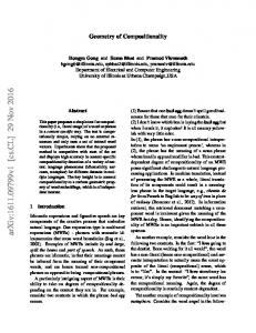
Upper bounds for g-leakages (bits) of the composed channel under 2-tries gain function

using a model similar to one of [24]. Although executions in Crowds can be infinite, a finite state model can be employed, keeping track of only the current forwarder instead of the full route. Then each element of the channel matrix can be computed by PRISM as the probability of reaching the corresponding state. The g-leakage of a single execution can be directly computed Maximum possible leakage from the channel; however, for multiple executions, the channel quickly becomes too big to be of practical use (already at 5 repetitions). On the other hand, gleakage can be bounded using the results in Section 4. The obtained Network topology changes every 2 observations bounds for up to 9 protocol repeNetwork topology changes every 3 observations Network topology never changes titions are shown in Fig. 3. Three Time (the number of observations) variations are given in which the topology changes every 2 execuFig. 3. Numbers of observations and bounds tions, every 3 executions or always stays the same. All bounds are computed using a uniform prior and some randomly generated channels. The experiments show that the compositionality technique allows us to obtain meaningful bounds when the system is too big to compute exact values. Note that the assumption of uniformly chosen forwarders is standard for the Crowds protocol, however it would be interesting to study how our results would change if we considered non-uniform distributions. For instance, we could have a non-uniform distribution if the possible forwarders were equipped with a notion of trust, like in [23]. We leave this for future work. 6.2

5

4

3

2

1

0

0

1

2

3

4

5

6

7

8

9

Evaluation on Randomly Generated Channels

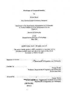
In this section we evaluate our bounds on min-entropy leakage using randomly generated channels. In particular, we evaluate the improvement on the bounds due to the input approximation technique, and the efficiency of our approach, which we have implemented as a library in leakiEst version 1.3 [1]. We first compare the exact leakage values with their upper bounds calculated using the input approximation technique in the case of shared input. Fig. 4 shows the average upper bounds obtained from Theorem 4, that can be applied when we know the channel matrix. Fig. 5 shows those obtained from Theorem 6 that we can apply when we do not know it. For both experiments we use randomly generated 10 × 10 channel matrices C and a prior π that contains some input with very small probabilities. We set ǫ = 0.1 in the first case and ǫ = V (π, C)/3 in the second one. We calculated the min-entropy leakage I∞ (π, C k C k C k C k C k C) (composition of six C’s), and its lower and upper bounds, using the n-ary generalizations of Theorems 4 and 6 (see Appendix for the precise formulations.) These cases give similar upper bounds as shown in Figs. 4 and 5. The xaxis represents noise levels of randomly generated matrices, which we define as 13

Min-entropy leakages (bits) of channels composed of 6 channels in parallel with shared input

Min-entropy leakages (bits) of channels composed of 6 channels in parallel with shared input

3

2.5

Upper bounds 2

1.5

1

Exact values

0.5

0

Lower bounds 0

0.05

0.1

0.15

0.2

Noise levels of randomly generated 10 ✕ 10 channel matrices

7

6

Upper bounds

5

4

3

Maximum possible leakage

2

Exact values 1

0

Lower bounds 0

0.05

0.1

0.15

0.2

Noise levels of randomly generated 10 ✕ 10 channel matrices

Upper bounds

2

1.5

Exact values 1

0.5

Lower bounds 0

0

0.05

0.1

0.15

0.2

Noise levels of randomly generated 10 ✕ 10 channel matrices

Fig. 5. Min-entropy leakages and their bounds for unknown channels Average upper bounds for min-entropy leakages (bits) of composed channels with shared input

Min-entropy leakages (bits) of channels composed of 6 channels in parallel with shared input

Fig. 4. Min-entropy leakages and their bounds for known channels

3

2.5

10

Upper bounds 8

Maximum possible leakage 6

4

2

Lower bounds 0

2

4

6

8

10

Numbers of components (different 100 ✕ 100 channels)

Fig. 6. Min-entropy leakages and their bounds when the analyst does not know the channels and chooses ǫ badly

Fig. 7. Upper bounds of min-entropy leakages as a function of the numbers of components

the maximum values (over rows of C) of the summations of the differences of probabilities from the uniform distributions. For instance, when the noise level is 0.10, the average upper bound is 1.699 in the first case (Fig. 4) while it is 1.701 in the second (Fig. 5). These upper bounds depend on how we choose the parameter ǫ for the input approximation technique. In particular upper bounds strongly depend on ǫ in the case of unknown channels. In Fig. 5 we chose ǫ = V (π, C)/3 which gives a relatively good upper bound. On the other hand, if we choose an ǫ too large we may obtain useless bounds. Indeed, if we set for instance ǫ = 0.2, then we obtain upper bounds above the maximum possible leakage, which is the min-entropy, and is always log 10 ≈ 3.322 (as shown in Fig. 6) since the input is shared. Fig. 7 shows average upper bounds of min-entropy leakages of randomly generated 100 × 100 channels, with randomly generated priors, noise level 0.1, and ǫ = 0.005. As we can see from the figure, the gap between the lower and upper bounds increases with the number of components. 14

Time (msec) to calculate upper bounds of min-entropy leakages of composed channels

Time (msec) to calculate the min-entropy leakage of the composed channel

4096

Exact min-entropy leakage values

2048

Upper bounds obtained with our approach

1024 512 256 128 64 32 16 8 4 2

0

1

2

3

4

5

6

7

1600

1400

1200

1000

800

600

400

200

0

0

20

40

60

80

100

The numbers of components (100 ✕ 100 channel matrices)

The numbers of components (randomly generated 10 ✕ 10 channel matrices)

Fig. 8. Average time to calculate minentropy leakages and their upper bounds

Fig. 9. Average time to calculate upper bounds as a function of the number of components

Finally we evaluate the efficiency of our method. We consider here the minentropy leakage. Fig. 8 shows the execution time on a laptop (1.8 GHz Intel Core i5) for leakiEst to compute the exact min-entropy leakages of the channels composed of randomly generated 10 × 10 component channels, in comparison with the time to compute their upper bounds. To compute the exact leakages, we used leakiEst with an option that calculates the leakages from exact matrices. As we can see, the execution time for the exact values increases rapidly. In fact, the size of composed channel increases exponentially with the number of components, so the complexity of this computation is at least exponential. For a large number of components, the time to calculate upper bounds increases linearly as shown in Fig. 9. As for the computation of the exact values with leakiEst, we expected an exponential blow-up, but we could not check it since we run out of memory because of the size of the matrices.

7

Conclusion and Future Work

We have investigated compositional methods to derive bounds on g-leakage. To improve the precision of the bounds, we have proposed a technique based on the idea of approximating priors by removing small probabilities up to a parameter ǫ. From our experimental results we have found that the dependency of the precision on ǫ is not straightforward. We leave for future work the problem of determining optimal values for ǫ. We also want to explore a possible relation between our technique and the notion of smooth entropies from the information theory literature [8]. This could allow us to develop a more principled approach to the input approximation technique.

References 1. leakiEst, http://www.cs.bham.ac.uk/research/projects/infotools/leakiest/

15

2. Alvim, M.S., Chatzikokolakis, K., Palamidessi, C., Smith, G.: Measuring information leakage using generalized gain functions. In: Proc. of CSF. pp. 265–279. IEEE (2012) 3. Andr´es, M., Palamidessi, C., van Rossum, P., Smith, G.: Computing the leakage of information-hiding systems. In: Proc. of TACAS. pp. 373–389 (2010) 4. Barthe, G., K¨ opf, B.: Information-theoretic bounds for differentially private mechanisms. In: Proc. of CSF. pp. 191–204. IEEE (2011) 5. Boreale, M.: Quantifying information leakage in process calculi. In: Proc. of ICALP. LNCS, vol. 4052, pp. 119–131. Springer (2006) 6. Boreale, M., Pampaloni, F., Paolini, M.: Asymptotic information leakage under one-try attacks. In: Proc. of FOSSACS. pp. 396–410 (2011) 7. Braun, C., Chatzikokolakis, K., Palamidessi, C.: Quantitative notions of leakage for one-try attacks. In: Proc. of MFPS. ENTCS, vol. 249, pp. 75–91. Elsevier (2009) 8. Cachin, C.: Smooth entropy and r´enyi entropy. In: EUROCRYPT. pp. 193–208 (1997) 9. Chatzikokolakis, K., Chothia, T., Guha, A.: Statistical Measurement of Information Leakage. In: Proc. of TACAS. pp. 390–404. LNCS, Springer (2010) 10. Chatzikokolakis, K., Palamidessi, C., Panangaden, P.: Anonymity protocols as noisy channels. Inf. and Comp. 206(2–4), 378–401 (2008) 11. Chatzikokolakis, K., Palamidessi, C., Panangaden, P.: On the Bayes risk in information-hiding protocols. J. of Comp. Security 16(5), 531–571 (2008) 12. Chothia, T., Kawamoto, Y., Novakovic, C., Parker, D.: Probabilistic point-to-point information leakage. In: Proc. of CSF. pp. 193–205. IEEE (June 2013) 13. Chothia, T., Kawamoto, Y.: Statistical estimation of min-entropy leakage (April 2014), http://www.cs.bham.ac.uk/research/projects/infotools/, manuscript 14. Chothia, T., Kawamoto, Y., Novakovic, C.: A tool for estimating information leakage. In: Proc. of CAV 2013 (2013) 15. Chothia, T., Kawamoto, Y., Novakovic, C.: LeakWatch: Estimating information leakage from java programs. In: Proc. of ESORICS 2014 (2014), to appear 16. Clark, D., Hunt, S., Malacaria, P.: Quantitative analysis of the leakage of confidential data. In: Proc. of QAPL. ENTCS, vol. 59 (3), pp. 238–251. Elsevier (2001) 17. Espinoza, B., Smith, G.: Min-entropy as a resource. Information and Computation (2013) 18. K¨ opf, B., Basin, D.A.: An information-theoretic model for adaptive side-channel attacks. In: Proc. of CCS. pp. 286–296. ACM (2007) 19. Kwiatkowska, M.Z., Norman, G., Parker, D.: PRISM 2.0: A tool for probabilistic model checking. In: Proc. of QEST. pp. 322–323. IEEE (2004) 20. Malacaria, P.: Assessing security threats of looping constructs. In: Proc. of POPL. pp. 225–235. ACM (2007) 21. Nassu, B., Nanya, T., Duarte, E.: Topology discovery in dynamic and decentralized networks with mobile agents and swarm intelligence. In: Proc. of ISDA. pp. 685– 690. IEEE (2007) 22. Reiter, M.K., Rubin, A.D.: Crowds: anonymity for Web transactions. ACM Trans. on Information and System Security 1(1), 66–92 (1998) 23. Sassone, V., Hamadou, S., Yang, M.: Trust in anonymity networks. In: CONCUR. pp. 48–70 (2010) 24. Shmatikov, V.: Probabilistic analysis of anonymity. In: Proc. of CSFW. pp. 119– 128. IEEE (2002) 25. Smith, G.: On the foundations of quantitative information flow. In: Proc. of FOSSACS. LNCS, vol. 5504, pp. 288–302. Springer (2009)

16

A

Extension to n Channels Composed in Parallel

A.1

The g-Leakages of Channels Composed in Parallel

Compositionality results on the parallel composition of two channels are extended to the case of n channels composed in parallel. The definitions of Mπmin and Mπmax are extended to n channels as follows. Definition 11. Let W = W1 × · · · × Wn , X = X1 × · · · × Xn and g be a joint gain function from W × X to [0, 1]. For i = 1, 2, · · · , n, let gi be a gain function from Wi × Xi to [0, 1]. Given an input distribution π on X , we define Mπmin and Mπmax : 1 )·...·πn [xk ]gn (wn ,xn ) Mπmin = minw∈W minx∈Sw π1 [x1 ]g1 (w1 ,xπ[x]·g(w,x) P 1 )·...·πn [xn ]gn (wn ,xn ) Mπmax = maxw∈W x∈Sw π1 [x1 ]g1 (w1 ,xπ[x]·g(w,x) .

where w = (w1 , w2 , · · · , wn ) and x = (x1 , x2 , · · · , xn ).

Then we obtain the following compositionality results. Theorem 7. For any jointly supported input distributions π on X and k channels (X1 , Y1 , C1 ), · · · , (Xn , Yn , Cn ), X

Igi (πi , Ci ) − log

i=1,2,··· ,n

A.2

X Mπmax M max Igi (πi , Ci ) + log πmin . ≤ Ig (π, C1 × · · · × Cn ) ≤ min Mπ Mπ i=1,2,··· ,n

The g-Leakage of Channels Composed in Parallel with Shared Input

Compositionality results on the parallel composition of two channels in the case of share input are also naturally extended to the case of n channels composed in parallel. For example, an upper bound of the g-leakage of a composed channel is given by: Theorem 8. For any input distribution π on X and k channels (X , Y1 , C1 ), · · · , (X , Yn , Cn ), Ig (π, C1 k · · · k Cn ) ≤

X

i=1,2,··· ,n

A.3


Ig (π, Ci ) + (n − 1) · Hgmin (π) − Hg (π) .

Input Approximation

Let π ′ = π|X \X ′ . Here are extensions of input approximation technique to n channels composed in parallel: 17

Corollary 6.     X M max′ V (π , C ) i i   − log ∞,π I∞ (πi , Ci ) − log min V (πi , Ci ) − ǫ M∞,π ′ i=1,2,··· ,n

≤ I∞ (π, C1 × · · · × Cn )     max X M∞,π ′ maxj=1,2,··· ,n V (πj , Cj )   I∞ (πi , Ci ) + log ≤ + log min . max V (π , C ) − ǫ M j=1,2,··· ,n j j ∞,π ′ i=1,2,··· ,n

P Corollary 7. I∞ (π, C1 k · · · k Cn ) ≤ i=1,2,··· ,n I∞ (πi , Ci ) + (n − 1) · (H min (π ′ ) −   maxj=1,2,··· ,n V (πj ,Cj ) . H∞ (π ′ ) + log maxj=1,2,··· ,n V (πj ,Cj )−ǫ

B B.1

Omitted Lemmas Decomposition of Channels

Sometimes it can be useful to decompose a large system for analysis purposes: the components may be easier to analyze than the whole system. Here, given a channel that outputs pairs in Y1 × Y2 , we consider the sub channels that output on Y1 and Y2 separately. Depending on whether we wish to perform an analogous separation also the inputs or not, we obtain two kinds of decomposition. Definition 12. (Decomposition) – The decomposition of a discrete channel (X1 ×X2 , Y1 ×Y2 , C) with respect to (X1 , Y1 ) and (X2 , Y2 ) is a pair of channels (X1 , Y1 , C|Y1 ) and (X2 , Y2 , C|Y2 ) where P P C|Y1 [x1 , y1 ] = x2 ∈X2 p(x2 |x1 ) y2 ∈Y2 C[(x1 , x2 ), (y1 , y2 )] P P C|Y2 [x2 , y2 ] = x1 ∈X1 p(x1 |x2 ) y1 ∈Y1 C[(x1 , x2 ), (y1 , y2 )].

– The decomposition of a discrete channel (X , Y1 × Y2 , C) with respect to Y1 and Y2 is a pair of channels (X , Y1 , C|Y1 ) and (X , Y2 , C|Y2 ) where P P C|Y1 [x, y1 ] = y2 ∈Y2 C[x, (y1 , y2 )] and C|Y2 [x, y2 ] = y1 ∈Y1 C[x, (y1 , y2 )].

For a composed channel (X1 ×X2 , Y1 ×Y2 , C1 ×C2 ), it is easy to prove that we have (C1 ×C2 )|Y1 = C1 and (C1 ×C2 )|Y2 = C2 . For a channel (X , Y1 ×Y2 , C1 kC2 ) with shared input, we have (C1 k C2 )|Y1 = C1 and (C1 k C2 )|Y2 = C2 . B.2

The Prior g-Entropies of Joint Input Distributions

The support Sw1 ,w2 , defined in Definition 8, satisfies the following property: Lemma 2. Let π be jointly supported, and g1 : W1 ×X1 → [0, 1], g2 : W2 ×X2 → [0, 1]. Then for all (x1 , x2 ) ∈ (X1 × X2 ) \ Sw1 ,w2 , π1 [x1 ] · g1 (w1 , x1 ) · π2 [x2 ] · g2 (w2 , x2 ) = 0. 18

Proof. Let (x1 , x2 ) ∈ (X1 × X2 ) \ Sw1 ,w2 . By definition, we have π[x1 , x2 ] · g((w1 , w2 ), (x1 , x2 )) = 0. Since π is jointly supported, π1 [x1 ] · π2 [x2 ] = 0. By the definition of joint gain functions, g1 (w1 , x1 )g2 (w2 , x2 ) = 0. Hence π1 [x1 ]g1 (w1 , x1 ) · π2 [x2 ]g2 (w2 , x2 ) = 0. The (prior) g-entropy Hg (π) of a joint input distribution π is lower-bounded by the summation of log Mπmin and the (prior) g-entropies of its two marginals π1 , π2 : Lemma 3. For any input distribution π on X1 × X2 , Hg (π) ≥ Hg1 (π1 ) + Hg2 (π2 ) + log Mπmin . Proof. Vg (π) · Mπmin =

X

max

π[x1 , x2 ] · g((w1 , w2 ), (x1 , x2 ))

(w1 ,w2 )∈W1 ×W2 (x1 ,x2 )∈X1 ×X2

·

≤

min

w1 ∈W1 ,w2 ∈W2

max

(w1 ,w2 )∈W1 ×W2

≤

min

(x1 ,x2 )∈Sw1 ,w2

 

X

π1 [x1 ]g1 (w1 , x1 ) · π2 [x2 ]g2 (w2 , x2 ) π[x1 , x2 ] · g((w1 , w2 ), (x1 , x2 ))

π[x1 , x2 ] · g((w1 , w2 ), (x1 , x2 ))

(x1 ,x2 )∈X1 ×X2

·

min

(x1 ,x2 )∈Sw1 ,w2

π1 [x1 ]g1 (w1 , x1 ) · π2 [x2 ]g2 (w2 , x2 ) π[x1 , x2 ] · g((w1 , w2 ), (x1 , x2 ))

X

max

π[x1 , x2 ]g((w1 , w2 ), (x1 , x2 )) (w1 ,w2 )∈W1 ×W2 (x1 ,x2 )∈Sw1 ,w2

·



π1 [x1 ]g1 (w1 , x1 )π2 [x2 ]g2 (w2 , x2 ) π[x1 , x2 ]g((w1 , w2 ), (x1 , x2 ))

(∵ For all (x1 , x2 ) ∈ (X1 × X2 ) \ Sw1 ,w2 , π[x1 , x2 ]g((w1 , w2 ), (x1 , x2 )) = 0.) ≤

(w1 ,w2 )∈W1 ×W2

=

X

max

max

(w1 ,w2 )∈W1 ×W2

= max

w1 ∈W1

X

π1 [x1 ]g1 (w1 , x1 ) · π2 [x2 ]g2 (w2 , x2 ))

(x1 ,x2 )∈X1 ×X2

X

π1 [x1 ] · g1 (w1 , x1 ) ·

π1 [x1 ] · g1 (w1 , x1 ) · max

w2 ∈W2

X

π2 [x2 ] · g2 (w2 , x2 )

x2 ∈X2

= Vg1 (π1 ) · Vg2 (π2 ). Therefore

π2 [x2 ] · g2 (w2 , x2 )

x2 ∈X2

x1 ∈X1

x1 ∈X1

X

Hg (π) = − log Vg (π) ≥ − log Vg1 (π1 ) − log Vg2 (π2 ) + log Mπmin = Hg1 (π1 ) + Hg2 (π2 ) + log Mπmin . 19

!

To obtain an upper bound for the g-entropy Hg (π) of a joint input distribution π, we assume that π is jointly supported. The upper bound is the summation of log Mπmax and the g-entropies of its two marginals π1 , π2 : Lemma 4. For any jointly supported input distribution π on X1 × X2 , Hg (π) ≤ Hg1 (π1 ) + Hg2 (π2 ) + log Mπmax . Proof. Vg (π) · Mπmax =

X

max

π[x1 , x2 ] · g((w1 , w2 ), (x1 , x2 ))

(w1 ,w2 )∈W1 ×W2 (x1 ,x2 )∈X1 ×X2

·

w1 ∈W1 ,w2 ∈W2

≥

π1 [x1 ]g1 (w1 , x1 ) · π2 [x2 ]g2 (w2 , x2 ) π[x1 , x2 ] · g((w1 , w2 ), (x1 , x2 ))

X

max

(x1 ,x2 )∈Sw1 ,w2



max

X



(w1 ,w2 )∈W1 ×W2

π[x1 , x2 ] · g((w1 , w2 ), (x1 , x2 ))

(x1 ,x2 )∈X1 ×X2

·

X



π1 [x1 ]g1 (w1 , x1 ) · π2 [x2 ]g2 (w2 , x2 )  π[x1 , x2 ] · g((w1 , w2 ), (x1 , x2 ))

(x1 ,x2 )∈Sw1 ,w2

≥

X

max

(w1 ,w2 )∈W1 ×W2

π1 [x1 ]g1 (w1 , x1 ) · π2 [x2 ]g2 (w2 , x2 )

(x1 ,x2 )∈Sw1 ,w2

X

π1 [x1 ]g1 (w1 , x1 ) (w1 ,w2 )∈W1 ×W2 (x1 ,x2 )∈X1 ×X2

=

=

=

max

max

(w1 ,w2 )∈W1 ×W2

max

w1 ∈W1

X

X

π1 [x1 ]g1 (w1 , x1 ) ·

π1 [x1 ]g1 (w1 , x1 )

X

!

·

= Vg1 (π1 ) · Vg2 (π2 ).

max

w2 ∈W2

(∵ Lemma 2) !

π2 [x2 ]g2 (w2 , x2 )

x2 ∈X2

x1 ∈X1

x1 ∈X1

· π2 [x2 ]g2 (w2 , x2 )

X

π2 [x2 ]g2 (w2 , x2 )

x2 ∈X2

Therefore Hg (π) = − log Vg (π) ≤ − log Vg1 (π1 ) − log Vg2 (π2 ) + log Mπmax = Hg1 (π1 ) + Hg2 (π2 ) + log Mπmax .

20

!

C

Omitted Proofs

In this section we present omitted proofs. C.1

Omitted Proofs from Section 3

Proposition 1. For any prior π, Mπmin > 0. Proof. Let π be any input distribution. Since probabilities and gains are nonnegative, it suffices to show that Mπmin 6= 0. Let w1 ∈ W1 , w2 ∈ W2 and (x1 , x2 ) ∈ Sw1 ,w2 . Then we have π[x1 , x2 ] 6= 0 and g((w1 , w2 ), (x1 , x2 )) 6= 0. Then, by the definition of joint gain functions, g1 (w1 , x1 )g2 (w2 , x2 ) 6= 0. In addition, we obtain π1 [x1 ] · π2 [x2 ] 6= 0 from π[x1 , x2 ] 6= 0. Hence π1 [x1 ]g1 (w1 , x1 ) · π2 [x2 ]g2 (w2 , x2 ) 6= 0 Therefore Mπmin 6= 0. Proof of Lemma 1 Vg (π, C1 ×C2 ) · Mπmin =

X

(y1 ,y2 )∈Y1 ×Y2

π[x1 , x2 ] (w1 ,w2 )∈W1 ×W2 (x1 ,x2 )∈X1 ×X2

·

≤

X

max

min

min

w1 ∈W1 ,w2 ∈W2

X

(x1 ,x2 )∈Sw1 ,w2



max

· (C1 ×C2 )[(x1 , x2 ), (y1 , y2 )] · g((w1 , w2 ), (x1 , x2 ))

π1 [x1 ]g1 (w1 , x1 ) · π2 [x2 ]g2 (w2 , x2 ) π[x1 , x2 ] · g((w1 , w2 ), (x1 , x2 ))

X

π[x1 , x2 ] (w1 ,w2 )∈W1 ×W2 (y1 ,y2 )∈Y1 ×Y2 (x1 ,x2 )∈X1 ×X2

X

max

≤

X

max

=

X X

≤



·

min

· (C1 ×C2 )[(x1 , x2 ), (y1 , y2 )] · g((w1 , w2 ), (x1 , x2 ))

(x1 ,x2 )∈Sw1 ,w2

π1 [x1 ]g1 (w1 , x1 ) · π2 [x2 ]g2 (w2 , x2 ) π[x1 , x2 ] · g((w1 , w2 ), (x1 , x2 ))

X

· π2 [x2 ]g2 (w2 , x2 ) · (C1 ×C2 )[(x1 , x2 ), (y1 , y2 )]

X

· π2 [x2 ]g2 (w2 , x2 ) · (C1 ×C2 )[(x1 , x2 ), (y1 , y2 )]

π1 [x1 ]g1 (w1 , x1 ) (w1 ,w2 )∈W1 ×W2 (y1 ,y2 )∈Y1 ×Y2 (x1 ,x2 )∈Sw1 ,w2

(∵ For all (x1 , x2 ) ∈ (X1 × X2 ) \ Sw1 ,w2 , π[x1 , x2 ]g((w1 , w2 ), (x1 , x2 )) = 0.)

π1 [x1 ]g1 (w1 , x1 ) (w1 ,w2 )∈W1 ×W2 (y1 ,y2 )∈Y1 ×Y2 (x1 ,x2 )∈X1 ×X2

y1 ∈Y1 y2 ∈Y2

=

y1 ∈Y1 y2 ∈Y2

=

X

max

(w1 ,w2 )∈W1 ×W2

X X





max

max

X

w1 ∈W1 x1 ∈X1

X

X

π1 [x1 ]C1 [x1 , y1 ] g1 (w1 , x1 ) ·

X

π2 [x2 ]C2 [x2 , y2 ] g2 (w2 , x2 )

x2 ∈X2

x1 ∈X1

π1 [x1 ]C1 [x1 , y1 ] g1 (w1 , x1 ) · max

π1 [x1 ]C1 [x1 , y1 ] g1 (w1 , x1 ) · 

w1 ∈W1 y1 ∈Y1 x1 ∈X1

= Vg1 (π1 , C1 ) · Vg2 (π2 , C2 ).

21

X

max

!

X

π2 [x2 ]C2 [x2 , y2 ] g2 (w2 , x2 )

X

π2 [x2 ]C2 [x2 , y2 ] g2 (w2 , x2 )

w2 ∈W2 x2 ∈X2



!

w2 ∈W2 y2 ∈Y2 x2 ∈X2



Therefore

Hg (π, C1 × C2 ) = − log Vg (π, C1 × C2 ) ≥ − log Vg1 (π1 , C1 ) − log Vg2 (π2 , C2 ) + log Mπmin = Hg1 (π1 , C1 ) + Hg2 (π2 , C2 ) + log Mπmin .

Vg (π, C1 ×C2 ) · Mπmax =

X

(y1 ,y2 )∈Y1 ×Y2

π[x1 , x2 ] (w1 ,w2 )∈W1 ×W2 (x1 ,x2 )∈X1 ×X2

·

≥

X

max

X

w1 ∈W1 ,w2 ∈W2

max

(y1 ,y2 )∈Y1 ×Y2

X

max

(w1 ,w2 )∈W1 ×W2

· (C1 ×C2 )[(x1 , x2 ), (y1 , y2 )] · g((w1 , w2 ), (x1 , x2 ))

π1 [x1 ]g1 (w1 , x1 ) · π2 [x2 ]g2 (w2 , x2 ) π[x1 , x2 ] · g((w1 , w2 ), (x1 , x2 ))

(x1 ,x2 )∈Sw1 ,w2

 

X

π[x1 , x2 ] · (C1 ×C2 )[(x1 , x2 ), (y1 , y2 )] · g((w1 , w2 ), (x1 , x2 ))

(x1 ,x2 )∈X1 ×X2

X

·

 π1 [x1 ]g1 (w1 , x1 ) · π2 [x2 ]g2 (w2 , x2 ) π[x1 , x2 ] · g((w1 , w2 ), (x1 , x2 ))

(x1 ,x2 )∈Sw1 ,w2

≥

X

(y1 ,y2 )∈Y1 ×Y2

X X =

max π1 [x1 ]g1 (w1 , x1 ) (w1 ,w2 )∈W1 ×W2 (x1 ,x2 )∈Sw1 ,w2

· π2 [x2 ]g2 (w2 , x2 ) · (C1 ×C2 )[(x1 , x2 ), (y1 , y2 )]

X

· π2 [x2 ]g2 (w2 , x2 ) · (C1 ×C2 )[(x1 , x2 ), (y1 , y2 )]

y1 ∈Y1 y2 ∈Y2

=

X

π1 [x1 ]g1 (w1 , x1 ) (w1 ,w2 )∈W1 ×W2 (x1 ,x2 )∈X1 ×X2

X X

y1 ∈Y1 y2 ∈Y2

=

max

(w1 ,w2 )∈W1 ×W2

X X

y1 ∈Y1 y2 ∈Y2



=

X

y1 ∈Y1

max

max

max

w1 ∈W1

X

X

X

X π2 [x2 ]C2 [x2 , y2 ] g2 (w2 , x2 ) π1 [x1 ]C1 [x1 , y1 ] g1 (w1 , x1 ) · x2 ∈X2

x1 ∈X1

π1 [x1 ]C1 [x1 , y1 ] g1 (w1 , x1 ) · max

w2 ∈W2

x1 ∈X1

 

π1 [x1 ]C1 [x1 , y1 ] g1 (w1 , x1 ) · 

w1 ∈W1 x1 ∈X1

= Vg1 (π1 , C1 ) · Vg2 (π2 , C2 ).

Therefore

(∵ Lemma 2) !

X

y2 ∈Y2

X

max

X



π2 [x2 ]C2 [x2 , y2 ] g2 (w2 , x2 )

w2 ∈W2 x2 ∈X2

Hg (π, C1 × C2 ) = − log Vg (π, C1 × C2 ) ≤ − log Vg1 (π1 , C1 ) − log Vg2 (π2 , C2 ) + log Mπmax = Hg1 (π1 , C1 ) + Hg2 (π2 , C2 ) + log Mπmax .

22

π2 [x2 ]C2 [x2 , y2 ] g2 (w2 , x2 )

x2 ∈X2

!

Proof of Theorem 1 Ig (π, C1 × C2 ) = Hg (π) − Hg (π, C1 × C2 ) ≤ Hg (π) − Hg1 (π1 , C1 ) − Hg2 (π2 , C2 ) − log Mπmin (By Lemma 1) ≤ (Hg1 (π1 ) − Hg1 (π1 , C1 )) + (Hg2 (π2 ) − Hg2 (π2 , C2 )) + log Mπmax − log Mπmin (By Lemma 1) = Ig1 (π1 , C1 ) + Ig2 (π2 , C2 ) + log

Mπmax Mπmin .

The other inequality is also proven using Lemma 1 in a similar way. Proof of Theorem 2 We instantiate Lemma 1 by taking g1 and g2 as g, π as π † and X1 = X2 = X : Hg (π † , C1 × C2 ) ≥ Hg (π1† , C1 ) + Hg (π2† , C2 ) + log Mπmin † . By π1† [x] = π2† [x] = π[x] for all x ∈ X , log Mπmin = −Hgmin (π) and Hg (π, C1 k † † C2 ) = Hg (π , C1 × C2 ), the theorem follows. Proof of Theorem 3 Ig (π, C1 k C2 ) = Hg (π) − Hg (π, C1 k C2 ) ≤ Hg (π) − Hg (π, C1 ) − Hg (π, C2 ) + Hgmin (π) (By Theorem 2) ≤ (Hg (π) − Hg (π, C1 )) + (Hg (π) − Hg (π, C2 )) −Hg (π) + Hgmin (π) = Ig (π, C1 ) + Ig (π, C2 ) + Hgmin (π) − Hg (π). Note that, since π is not necessarily jointly supported, we cannot instantiate Lemma 1 (and cannot obtain a lower bound for the leakage). C.2

Omitted Proofs from Section 4

Proof of Corollary 3 By taking g, g1 , g2 as identity gain functions, Hg (π1 × π2 , C1 × C2 ) = H∞ (π1 × π2 , C1 × C2 ), Hg1 (π1 , C1 ) = H∞ (π1 , C1 ), Hg2 (π2 , C2 ) = H∞ (π2 , C2 ), Mπmin = min max M∞,π and Mπmax = M∞,π . Then the first claim follows from the first claim of Lemma 1 and the second claim follows from the second. min max If π1 and π2 are independent we have M∞,π = M∞,π = 1, hence the last claim follows. Proof of Corollary 4 By taking g, g1 , g2 as identity gain functions, Ig (π1 × π2 , C1 × C2 ) = I∞ (π1 × min π2 , C1 × C2 ), Ig1 (π1 , C1 ) = I∞ (π1 , C1 ), Ig2 (π2 , C2 ) = I∞ (π2 , C2 ), Mπmin = M∞,π 23

max and Mπmax = M∞,π . Then the first and second claims follow from Theorem 1 and Corollary 2 respectively.

Proof of Corollary 5 When w = x, π[x]gid (w, x) = π[x] holds . Hence Hgmin (X) = H min (X). id By definition, Hgid (π, C1 k C2 ) = H∞ (π, C1 k C2 ), Hgid (π, C1 ) = H∞ (π, C1 ), Hgid (π, C2 ) = H∞ (π, C2 ) and Hgid (π) = H∞ (π). Then the claims follow from Theorems 2 and 3.

C.3

Omitted Proofs from Section 5

Proof of Theorem 4 X max π[x]C[x, y] V (π, C) = y∈Y

x∈X

X

X

′

′

!

π[x ]C[x , y]    X X X π[x′ ] C[x′ , y] max ′ π[x]C[x, y] + =

≤

y∈Y

y∈Y

=

X

y∈Y

max π[x]C[x, y] +

x∈X \X ′

x′ ∈X ′

x∈X \X

x′ ∈X ′

y∈Y



max π[x]C[x, y] + ǫ

x∈X \X ′

= V (π|X \X ′ , C) + ǫ.

By maxx∈X \X ′ π[x] = maxx∈X π[x], we have V (π|X \X ′ ) = V (π). Then V (π, C) V (π|X \X ′ ) V (π|X \X ′ , C) + ǫ ≤ log V (π|X \X ′ )   V (π|X \X ′ , C) V (π|X \X ′ , C) + ǫ = log · V (π|X \X ′ ) V (π|X \X ′ , C)   ǫ . = I∞ (π|X \X ′ , C) + log 1 + V (π|X \X ′ , C)

I∞ (π, C) = log

On the other hand, by V (π|X \X ′ , C) ≤ V (π, C), we obtain I∞ (π|X \X ′ , C) ≤ I∞ (π, C). Proof of Theorem 5 By the first claim in the proof for Theorem 4, V (π ′ , C1 ×C2 ) ≥ V (π, C1 ×C2 )−ǫ ≥ 24

max(V (π1 , C1 ), V (π2 , C2 )) − ǫ. Then I∞ (π, C1 × C2 )  ≤ I∞ (π ′ , C1 × C2 ) + log 1 +  ≤ I∞ (π ′ , C1 × C2 ) + log 1 + ≤ I∞ (π1′ , C1 ) + I∞ (π2′ , C2 ) +

ǫ V

(π ′ ,C

1 ×C2 )





ǫ max(V (π1 ,C1 ),V (π  2 ,C2 ))−ǫ  Mπmax max(V (π1 ,C1 ),V (π2 ,C2 ) ′ log M min + log max(V (π1 ,C1 ),V (π2 ,C2 ))−ǫ ′ π

≤ I∞ (π1 , C1 ) + I∞ (π2 , C2 ) + log

Mπmax ′ Mπmin ′

+ log



(By Corollary 4)

max(V (π1 ,C1 ),V (π2 ,C2 ) max(V (π1 ,C1 ),V (π2 ,C2 ))−ǫ

(By Theorem 4)

The other inequality is shown as follows. I∞ (π, C1 × C2 ) ≥ I∞ (π ′ , C1 × C2 ) ≥ I∞ (π1′ , C1 ) + I∞ (π2′ , C2 ) − log ≥ I∞ (π1 , C1 ) + I∞ (π2 , C2 ) − log ≥ I∞ (π1 , C1 ) + I∞ (π2 , C2 ) − log

Mπmax ′ Mπmin ′ max Mπ ′ Mπmin ′ Mπmax ′ Mπmin ′

(By Theorem 4) (By Corollary 4)     ′ V (π ′ ,C1 )+ǫ 2 )+ǫ − log V (π′ ,C1 ) − log VV(π(π,C ′ ,C ) 2 − log



V (π,C1 ) V (π,C1 )−ǫ

4)  (By Theorem  V (π,C2 ) − log V (π,C2 )−ǫ ✷

Proof of Theorem 6 Let π ′ = π|X \X ′ . Then by Theorem 4, I∞ (π, C1 k C2 )   ≤ I∞ (π ′ , C1 k C2 ) + log 1 + V (π′ ,Cǫ 1 kC2 )   max(V (π1 ,C1 ),V (π2 ,C2 )) ≤ I∞ (π ′ , C1 k C2 ) + log max(V (π1 ,C1 ),V (π2 ,C2 ))−ǫ

≤ I∞ (π1 , C1 ) + I∞ (π2 , C2 ) + H min (π ′ ) − H∞ (π ′ ) +

25





max(V (π1 ,C1 ),V (π2 ,C2 )  max(V (π1 ,C1 ),V (π2 ,C2 ))−ǫ  max(V (π1 ,C1 ),V (π2 ,C2 ) log max(V (π1 ,C1 ),V (π2 ,C2 ))−ǫ

≤ I∞ (π1′ , C1 ) + I∞ (π2′ , C2 ) + H min (π ′ ) − H∞ (π ′ ) + log