Comprehensive framework for gradient-based ... - Stanford University

Computational Geosciences manuscript No. (will be inserted by the editor)

Comprehensive framework for gradient-based optimization in closed-loop reservoir management Vladislav Bukshtynov · Oleg Volkov · Louis J. Durlofsky · Khalid Aziz

Received: date / Accepted: date

Abstract An efficient, robust and flexible adjoint-based computational framework for performing closed-loop reservoir management is developed and applied. The methodology includes gradient-based production optimization and data assimilation (history matching). Flexibility is achieved through use of automatic differentiation (AD) within the reservoir simulation, production optimization and history matching modules. The use of AD will also facilitate the application of closed-loop reservoir management to physical models of higher complexity. A fast sequential convex programming (SCP) solver based on the method of moving asymptotes (MMA) is applied for the production optimization component of the closed-loop. This technique is shown to outperform the sequential quadratic programming (SQP) method, which is commonly used for production optimization computations. The history matching component of the workflow integrates both production data and proxy seismic measurements into a unified adjoint-based data assimilation framework. The effect of noisy data, and data of different types, on the accuracy of the history matching component is assessed. The overall closed-loop reservoir management methodology is tested using the well-documented Brugge model. Results demonstrate the efficient performance of the

V. Bukshtynov (B) · O. Volkov · L. J. Durlofsky · K. Aziz Department of Energy Resources Engineering, Stanford University, Stanford, CA 94305-2220, USA E-mail: [email protected]

O. Volkov E-mail: [email protected] L. J. Durlofsky E-mail: [email protected] K. Aziz E-mail: [email protected]

individual closed-loop components and the improvement in net present value that is achieved using these procedures. Keywords Closed-loop reservoir management · Production optimization · History matching · Seismic data · Noisy data · Gradient-based optimization · Adjoint formulation · Automatic differentiation · PCA-based parameterization

1 Introduction The reservoir modeling and optimization capabilities that have been developed in recent years hold great promise for improving reservoir performance. Closed-loop reservoir management (CLRM) is one such strategy. CLRM, which has been widely studied [3, 7, 15, 19–21, 27, 37, 44], essentially involves periodic history matching and production optimization computations. Various minimization procedures have been applied for these computations, though our emphasis here will be on gradient-based methods, with gradients computed using adjoints for both history matching and production optimization. CLRM is illustrated schematically in Figure 1. The production system includes the field and facilities, in which production and seismic data are collected periodically. These data are then used for the model update step, in which the geological model or models are adjusted such that the predicted reservoir response closely matches the actual data. Time-varying optimal well settings (flow rates or bottomhole pressures) are then determined based on this updated geological model. Hydrocarbon production using these controls proceeds until the next closed-loop step, at which time the geological model is again updated and the optimal controls recomputed. The loop is repeated for the duration of the production time frame. Because the geological model may be highly uncertain at early stages of production, the model

2

Vladislav Bukshtynov et al.

and controls can change significantly during the course of CLRM.

Production Production System system

Controls Controls

Production Data Data

Optimization Optimization

Update Geological Detailed Model Model

Seismic Data

Update

Gradient Reduced Framework Model

Fig. 1 Closed-loop reservoir management scheme.

The two areas most relevant to CLRM are production optimization and data assimilation. The literature associated with both of these fields is very extensive, so our focus here will be on papers that are directly relevant to this study. A recent review of history matching procedures can be found in [29]. As noted above, our interest here is in gradientbased history matching, discussed in, e.g., [25,30,37]. These methods are very efficient if adjoint procedures are used to construct gradients. In this paper, our adjoint-based history matching scheme utilizes both production and seismic data. Many previous researchers (e.g., [8–10, 12, 18, 31, 38, 41]) have considered the combined use of production and seismic data, but little previous work has involved the application of a general adjoint-gradient procedure for both production and seismic data, as is presented here. We also introduce a simple procedure for generating proxy seismic data with spatial filtering and varying degrees of noise, and the impact of noise on the quality of the history matched solution is assessed. Gradient-based production optimization has also been addressed in a number of recent papers; e.g., [2,3,24,27,35, 37, 43, 44]. See [20] for a comprehensive description of this general area and an extensive literature review. An important aspect of our work is the choice of an efficient nonlinear programming solver to ensure computational efficiency in the production optimization component of the closed-loop scheme. Specifically, we compare a state-of-the-art SQP solver with an SCP solver based on MMA [39]. The former is commonly used in production optimization [24, 37], though the latter does not appear to have been previously applied in this application area. The automatic differentiation procedure used in this work enables us to obtain adjoint-based gradients for both

production optimization and history matching. The AD technique has been implemented into Stanford’s Automatic Differentiation-based General Purpose Research Simulator, AD–GPRS, using the Automatic Differentiation Expression Templates Library (ADETL). This procedure was originally developed in [45, 46] and later extended in [47, 48]. This paper proceeds as follows. In the next section we give the mathematical details of the CLRM scheme. The production optimization and history matching components are cast as optimization problems that are solved using an adjoint gradient algorithm. Computational aspects of the methodology, including the optimization software, are described in Section 3. In Section 4 we present a range of computational results for the synthetic Brugge model. These results entail the use of both production and 4D (time–lapse) seismic data. Concluding remarks are provided in Section 5.

2 Mathematical description 2.1 Reservoir simulation model Although our formulation is quite general, we describe our model here in terms of an isothermal oil-water flow problem. The general set of governing partial differential equations (PDEs) can be expressed as g(x, u) = 0, x(t0 ) = x0 ,

(1)

t ∈ [t0 ,t f ]. Here t is time, x denotes the state variables (phase pressure p p and saturation s p in this case), and u represents model parameters (for history matching) or well control parameters (for production optimization). The first equation in (1) is a standard mass balance equation for component/phase p, with p = o, w, which designate oil and water (see, e.g., [1])

∂ (ϕ ρ p s p ) + div (ρ p v p ) + ρ p q p = 0, p = o, w. ∂t

(2)

Here the phase flux v p is given by Darcy’s law v p = −k

krp (∇p p − γ p ∇D) . µp

(3)

The phase dependent parameters appearing in (2)–(3) are molar density ρ p , relative permeability krp , viscosity µ p , vertical pressure gradient γ p = ρ p g, and source term q p . The space dependent parameters are porosity ϕ , absolute permeability k, and vertical depth D. The system is closed by the relation so + sw = 1 and a capillary pressure relationship (if capillary effects are included; otherwise po = pw ). We reiterate that, although the above equations are for an oilwater system, the implementation can handle general compositional problems.

Comprehensive framework for gradient-based optimization in closed-loop reservoir management

In the discretized model, the total volumetric phase flow rate in well j (q j,p ), and the phase flow rate in completion i in well j (qij,p ), are given by q j,p = ∑ qij,p , i

requires the Gˆateaux differential of the objective function (5), defined as J (u + ε · δ u) − J (u) , ε →0 ε

dJ (u; δ u) , lim

j = 1, . . . , Nwell ,

) ( ) krp ( i qij,p = T w p − pwj − ρ j ∆ z . µp i

3

(4)

to vanish for all perturbations δ u [26], i.e., ˆ δ u) = 0, dJ (u;

Here T w represents the well transmissibility factor (well index), pi is the well-block pressure, and pwj + ρ j ∆ z is the wellbore pressure at the corresponding location. The latter involves the well bottom-hole pressure (BHP) pwj , which is defined at a reference depth z0 , along with the adjustment ρ j ∆ z, which accounts for the difference in wellbore pressure between the reference and cell-center depth (here ρ j is the average density of the fluid in the wellbore). Note that, for simplicity, frictional and other pressure losses in the wellbore are neglected.

∀ δ u.

In (9), u0 is the initial guess corresponding to an approximation of u, and τ (m) is the length of the step in the search direction at iteration m. In the simplest case, the search direction

CLRM entails solving two types of optimization problems sequentially. We defer the detailed description of these problems to Section 2.8, and the adjoint gradient solution algorithm to Sections 2.4 and 2.5. Here, we consider an optimization problem in a general form, with the objective function defined as

t0

F(t, x, u) dt.

(5)

Here F(t, x, u) is a nonlinear function whose form, for production optimization and history matching problems respectively, will be specified in Sections 2.8.1 and 2.8.2. The optimal solution uˆ is obtained through minimization or maximization of the objective function J (x, u) as follows: uˆ = argmin J (x, u),

(6a)

production optimization: uˆ = argmax J (x, u),

(6b)

history matching:

(10)

v

2.2 Optimization problems

∫ tf

(8)

Due to its complexity the equality (8) is solved iteratively uˆ = limm→∞ u(m) , where { (m+1) u = u(m) + τ (m) δ u(m) , m = 1, . . . , (9) u(1) = u0 .

δ u(m) = argmin dJ (u(m) ; v)

J (x, u) =

(7)

u

u

subject to the reservoir flow equations (1) and any applicable constraints that define a feasibility region for u. The details of the constraint treatment are provided in Section 2.7. Note that in the optimization problems (6a) and (6b) the state variables x are considered to be dependent on u through an implicit relationship defined by (1). A proper treatment of this relationship is discussed in Section 2.4. Solutions to the problem (6) in general are located either at an extremum or on the boundary of the feasibility region. We postpone the feasibility discussion until Section 2.7 and consider the algorithm for finding extrema. These points are characterized by the first-order optimality condition, which

represents the steepest descent direction. However, a more efficient search is achieved through use of advanced minimization/maximization techniques. In this work, we employ two dedicated SCP algorithms, discussed in Section 2.3, to handle the τ (m) δ u(m) term in (9). Note that, since the optimization problem (6) is in general nonconvex, condition (8) ˆ characterizes only a local, rather than the global, optimum u. However, because SCP solvers accumulate search direction information from a number of iterations, the trust region is larger, and the optimal solution “less” local, than in steepest descent. We now discuss SCP in more detail.

2.3 Sequential convex programming (SCP) An SCP algorithm finds an optimum uˆ by solving a sequence of convex programming (CP) problems where an objective function is replaced by its convex approximation. The CP problems are solved at each iteration m to determine the update τ (m) δ u(m) in (9) within the feasibility region of the optimization variable space. When the optimization problem is known to have a nonunique solution, the success of SCP relies on the characteristics of the trust region and the ability to define and solve individual CP problems with minimal computational effort. Commonly used approximations are those obtained with Taylor expansions. Approximations of order higher than two are not used in production optimization and history matching because of their prohibitive computational cost. The linear approximation is not applied directly because, due to the nonlinearity of these problems, it leads to a small trust region. However, it often serves as a building block for other

4

convex approximations that depend on the exact sensitivity of the objective function with respect to the optimization variables. In the next section we provide a detailed description of the adjoint gradients, which provide the most accurate estimation of this sensitivity. The quadratic expansion within the sequential quadratic programming algorithm has proven to be highly efficient for production optimization and history matching [24, 37]. The computational efficiency of SQP is achieved by using the adjoint gradients to construct both linear and quadratic terms in the approximation, along with a dedicated optimization algorithm to solve a quadratic problem. The quadratic term accumulates the gradient information from multiple optimization iterations. Therefore, the quadratic approximation can have an arbitrarily large trust region and can thus avoid some local minima. Depending on the form of the objective function and the initial guess, this capability could have positive or negative consequences. A common observation is that SQP, though quite general, requires some amount of tuning for a particular optimization problem. Dedicated SCP algorithms that use convex approximations consistent with the particular nonlinear form of the objective function have been developed in many application areas. Among these, the reconstruction of the geometrical scaling factors in structural optimization resembles the mathematical formulation of the production optimization problem with BHP controls. This similarity is due to the separability and quasi-linearity of the objective function and PDE constraints with respect to individual optimization variables (i.e., partial Hessians Juu and guu are diagonal or zero in both problems). In this situation, the use of convex approximations based on the linearization of functions with respect to reciprocal optimization variables enhances the convergence properties of the optimization procedure [14]. A successful modification of this approach, called method of moving asymptotes (MMA) [39], uses an approximation of J in the vicinity of u¯ in the form [ ] (Ui − u¯i )2 e ¯ + ∑ ∇Ji J (u) = J (u) − (Ui − u¯i ) Ui − ui i ∈ I+ (11) [ ] (u¯i − Li )2 − ∑ ∇Ji − (u¯i − Li ) , (ui − Li ) i ∈ I− where ui designates a component of the vector u, ∇Ji is a component of the gradient of the objective function J , Ui and Li are tunable parameters, I+ = {i : ∇Ji > 0}, and I− = {i : ∇Ji < 0}. In (11), Li and Ui are adjusted such that Je > J at the minimum of Je, and Je < J at the maximum of Je, for minimization and maximization problems respectively. This treatment is applied to stabilize and accelerate the convergence of the optimization process [14]. In this method, Li and Ui act as asymptotes that change the curvature of the approximation Je(u). Their initial values are set

Vladislav Bukshtynov et al.

to the lower and upper bounds of the optimization variables ¯ In the case of a quasi-linear objective function, the ability u. to adjust the curvature from the beginning of the optimization process plays an important role. If Li and Ui are chosen ¯ then Je(u) has small curvature in a large “far away” from u, ¯ which allows the optimizer to take large neighborhood of u, steps at the beginning of the optimization process. 0

0 Li

Ui

−0.05

Li

Ui solution after 1 iteration

−0.05

initial guess

−0.1

−0.1

optimal solution

−0.15 2

3

4

5

6

−0.15 7

2

(a) MMA, 1st iteration

3

4

5

6

7

(b) MMA, 2nd iteration

0

0

initial guess

−0.05

−0.05

−0.1

−0.1

−0.15

−0.15

optimal solution 2

3

4

5

(c) SQP, 1st iteration

6

7

solution after 1 iteration 2

3

4

5

6

7

(d) SQP, 2nd iteration

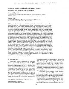
Fig. 2 (a, b) illustrate the adjustment of asymptotes in MMA. The first two iterations of MMA are compared with a trust region method (SQP) in (c, d). All figures show the objective function (black line), and the convex approximation before (thick blue line) and after (thick red line) adjustment used by the optimizer. In (a), MMA asymptotes before (vertical blue dashed line) and after (vertical red dashed lines) adjustment are shown. In (b), neither the convex approximation nor the asymptote requires adjustment.

The advantages of MMA relative to SQP can be illustrated as follows. In SQP, the curvature of the initial approximation of J is assigned with a default constant value, since at this point we only have a unique instance of the gradient, which does not allow us to approximate the Hessian. The optimization process requires a certain number of iterations before a working approximation of the Hessian is constructed. In MMA, by contrast, the curvature of the approximation of J at the point u¯ is directly controlled by the values of Li and Ui . Therefore a suitable curvature is available at the first optimization iteration. Figure 2 illustrates in a simple fashion this adjustment of the curvature. The example involves a minimization problem in one variable. It entails two iterations of MMA, which are compared with two iterations of SQP (namely the trust region SQP). The MMA optimization is started with an initial approximation (thick blue line) shown in Figure 2(a). At the first iteration, the minimum of the approximation function is below the objective function. The asymptotes (verti-

Comprehensive framework for gradient-based optimization in closed-loop reservoir management

cal dashed lines) are then shifted to produce a new approximation (thick red line). At the second MMA iteration, the minimum of the approximation (thick red line) is above the objective function, so no shift in the asymptotes is needed. Note that MMA is a trust region method, i.e., it does not perform a line search. However it is proven in [49] that MMA converges from any initial guess. MMA is also often more efficient computationally than SQP. This is because a solution of the convex programming problem in MMA is readily available. In addition, MMA requires fewer resources than SQP to store the approximation. A major disadvantage of MMA relative to SQP, however, is that it relies on a particular form of the objective function and regularization (if any). For example, in the history matching problem, the curvature of the objective function is less prone to changes because of the need to maintain geological consistency in the reservoir parameters. For this reason MMA, which significantly alters the curvature of the approximation to fit the objective function, demonstrates poor performance for the history matching problem, in contrast to the production optimization problem.

2.4 Adjoint-based gradients For PDE-constrained optimization problems, we must account for the implicit relationship (1) between state and control variables. This is accomplished by estimating sensitivities of the objective functions with respect to the PDE constraints, called adjoint variables [28]. One of the most efficient ways to obtain these sensitivities is through an augmented objective function called the Lagrangian L, which shares the same extrema as the original objective function J (x, u) L(x, u, λ ) = J (x, u) + ⟨λ , g(x, u)⟩,

(12)

where λ are the Lagrange multipliers for g(x, u) and ⟨·, ·⟩ denotes the inner product. At this stage, we eliminate the PDE constraint (1) at the cost of increasing the space of the optimization variables with λ . After requiring that the partial derivatives of the Lagrangian (12) with respect to λ , x and u vanish, we obtain the first optimality conditions, which are, respectively

where gx and gu correspond to the linearization of the state equation (1) with respect to x and u. Equations (13)–(15) are solved sequentially in the following manner. The state variables x are computed first from (13), after which the adjoint variables λ are found from adjoint equation (14). Equation (15) is then used to update control variables u. This equation is not solved explicitly. Instead, it defines a linear relation between a perturbation δ u and the total variation of L, also known as the Fr´echet derivative dL = ⟨Ju (x, u) + λ gu (x, u), δ u⟩.

(13)

• adjoint equation

λ gx (x, u) = −Jx (x, u),

(14)

Algorithm 1 Adjoint gradient workflow for a general optimization problem m←1 u(1) ← initial guess u0 repeat given estimate of u(m) , solve state equations (13) for x(m) given x(m) and u(m) , solve adjoint equations (14) for λ (m) update u(m+1) using (9) with a descent/ascent direction derived from the gradient ∇u J , Ju (x(m) , u(m) ) + λ (m) gu (x(m) , u(m) )

(15)

(17)

m ← m+1 until the termination criteria are satisfied to a given tolerance

2.5 Discrete formulation Let us assume that, as is typical in reservoir simulation, (1) is discretized in space using a finite volume procedure and in time using the backward Euler (fully implicit) scheme. This results in a nonlinear algebraic system of equations gn (xn , xn−1 , un ) = 0, x0 = x(t0 ),

(18)

where xn = x(tn ), n = 1, . . . , N, is the discretized state variable at the end of time step n (which is of size ∆ tn ). The AD-GPRS solution procedure for solving (18), for multiphase, multicomponent flow, is described in [47]. The continuous objective function (5) is approximated by a first-order scheme

• optimization equation

λ gu (x, u) = −Ju (x, u),

(16)

The first term of the inner product in (16) is called the adjoint gradient. It is independent of δ u and points in the direction of the steepest ascent of L. This property is also utilized to choose between the nearest maximum or minimum. Algorithm 1 summarizes the steps in the adjoint gradient approach for a general optimization problem.

• state equation (the same as (1)) g(x, u) = 0,

5

J (x, u) =

N

∑ ∆ tn Fn (tn , xn , un ) + O (max {∆ tn }) .

n=1

(19)

6

Vladislav Bukshtynov et al.

Following the steps described in Section 2.4, the discrete adjoint gradient with respect to control variables un is given by ) N ( ∂ Fn ∂ gn ∇ u J = ∑ ∆ tn + λ Tn , (20) ∂ un ∂ un n=1 where the discrete adjoint variables λ n satisfy ( ) ∂ Fn T ∂ gn T ∂ gn+1 λn = − λ n+1 + ∆ tn , ∂ xn ∂ xn ∂ xn ∂ gN ∂ FN λ TN = −∆ tN , n = 1, 2, . . . , N − 1. ∂ xN ∂ xN

(21)

Here and throughout this paper, (·)T denotes transpose. More details on the derivation of (20) and (21) can be found in [34].

2.6 Automatic differentiation As should be clear from our discussion above, the use of discrete adjoint gradients (20) is the key component of our CLRM procedure. This approach is appropriate for CLRM as it (1) provides all partial derivatives in (20)–(21) based on the numerical solution of the reservoir and adjoint equations (13)–(14), and (2) does not lead to excessive overhead or restrictions on the solution of the reservoir equations themselves. It is important to note that the use of adjoints is much more efficient than obtaining numerical partial derivatives of the functions Fn and gn with respect to state and control variables using a finite difference scheme, which becomes very expensive as the number of optimization variables increases. Analytical differentiation has traditionally been used within reservoir engineering to construct the adjoint equations. This requires access to source code and detailed calculations and coding, which are prone to error. In addition, when updating or enhancing the capabilities of the forward simulation model, the detailed adjoint treatment must be revisited. Due in part to its ability to overcome the problems mentioned above, automatic differentiation is gaining popularity in scientific and high performance computing. On the one hand, it allows analytical, i.e., exact and fast, evaluation of the partial derivatives of all nonlinear functions and quantities involved in the formulation of the reservoir equations. On the other hand, any new physics added to the existing reservoir model is automatically taken into account. The novelty of our computational approach applied to CLRM involves utilizing AD in obtaining gradients for both the production optimization and history matching components. We note that AD was used in previous work for the computation of gradients for production optimization in compositional simulation [24].

The reservoir equations are in general PDEs of parabolic type. Therefore, their adjoints are also parabolic, and are solved backward in time as seen in (21). Thus, the reservoir equations and their adjoints must be solved sequentially. One approach would be to store all partial derivatives employed in (21), which amounts approximately to Nvar × Nvar × N floating point numbers, where Nvar is the total number of state variables obtained after spatial discretization and N is the number of time steps in the discrete reservoir model (18). In addition, since the terms ∂ Fn /∂ xn , ∂ Fn /∂ un , ∂ gn /∂ un are not required in the forward simulation, computing and storing them will unavoidably slow down the process. Our AD-based reservoir simulator AD– GPRS adopts a different approach by storing only the state variables, enumerated to approximately Nvar × N, and reassembling the residual gn and the constitutive parts of J as required. The optimization module in AD–GPRS and the AD framework itself ensure the fidelity of this reassembly. In addition, the framework is customized to adapt to changes in the optimization variables caused, for example, by changes in well controls during the simulation (e.g., switches from BHP to rate control). 2.7 Handling bounds and constraints Most of the optimization parameters in CLRM are subject to limitations. For example, BHPs and flow rates are restrained by technical limits on the wells and facilities. The geological model parameters such as permeability and porosity are constrained to fall within physical ranges. In the optimization problems these limitations are translated into bounds on the optimization variables u, which are satisfied by the optimizer. If a particular limitation is not applied directly to an optimization variable, it enters as a nonlinear output constraint. This is the case, for example, for constraints on phase flow rates when the well control is BHP. In this situation, constraints can be satisfied either during the simulation or within the optimization [24, 35]. Numerical studies [24, 43] have shown that, when using an SQP solver, it is often advantageous to enforce the constraints during the simulation (even though this requires the use of some heuristics) rather than in the optimization. In this work, we apply an approach related to that in [24] and proceed as follows. For purposes of illustration, assume we have a production well operating under BHP control (with maximum and minimum BHP bounds specified) that is subject to a maximum water rate constraint. The production optimization module will have provided the target BHP for the time step under consideration. If the use of this BHP does not lead to a violation of the water rate constraint at the current Newton iteration, then this BHP acts as the control. If, however, this target BHP does lead to a violation of the water rate constraint at the current Newton iteration,

Comprehensive framework for gradient-based optimization in closed-loop reservoir management

then we perform an approximate test to assess whether or not the well can operate under water rate control, with the target given by the maximum water rate constraint, while not having the BHP fall below the value determined by the optimizer. If the test indicates that the rate control specification is feasible (with respect to BHP), then the well is operated under rate control. If rate control is infeasible, then the well is shut in for this Newton iteration. Analogous procedures are applied for other production and injection well constraints. It is important to note that wells can also be shut in during an AD–GPRS run when back flow occurs; i.e., when a zone intersected by the injector actually produces into the well or a zone intersected by a producer actually injects fluid into the reservoir.

7

/ where δ (tn − τk ) = 1 ∆ tn is the first-order approximation of the Dirac delta function. The particular form of fk depends on the type of measured data, namely • well production rate data q

Nwell N p

fk (xn , u) =

∑ ∑ C j,p (q j,p − q˜ j,p )2 ,

• well BHP data BHP Nwell

fk (xn , u) =

∑ Cj

(

pBHP − p˜BHP j j

)2

,

(26)

j=1

• time-lapse seismic data, e.g., phase saturation s p , given by a seismic inversion or a proxy of seismic observations Nblock N p −1

2.8 Objective functions

(25)

j=1 p=1

fk (xn , u) =

∑ ∑

C p (s j,p − s˜ j,p )2 ,

(27)

j=1 p=1

2.8.1 Production optimization The objective function used in this work for production optimization is net present value (NPV). The discretized cashflow appearing in the objective function (19) as the term Fn is expressed as Fn (tn , xn , un ) =

Nwell N p

∑ ∑ C j,p (tn ) q j,p (xn , un ),

(22)

j=1 p=1

where q j,p and C j,p denote respectively the volumetric production/injection flow rate and discounted price of phase p in well j, and N p designates the number of phases. Note that in production optimization the objective function (19) is implemented in the problem (6b).

where coefficients C j,p , C j , C p are diagonal elements of matrix CD−1 , q j,p , pBHP and s j,p designate simulated phase proj duction rates, well BHPs and phase saturation, and q˜ j,p , p˜BHP and s˜ j,p indicate the corresponding observed quantij q BHP are the numbers of wells providties. Here Nwell and Nwell ing phase production rate and BHP data, respectively, while Nblock is the number of reservoir grid blocks where seismic measurements are available. Well flow rates for different phases can differ substantially. We address this by changing volumetric rates to mass rates for production wells and by scaling the various contributions to J (xn , u). Specifically, (25) is replaced by q

Nwell N p

fk (xn , u) =

∑ ∑ C j,p D2p (q j,p − q˜ j,p )2 ,

(28)

j=1 p=1

2.8.2 History matching

where D p is a phase relative density defined as follows

When solving the history matching problem (6a), the model parameters u are grid-block or interface properties of the discrete reservoir, e.g., porosity, permeability, or interblock transmissibility. It is common to define an objective function in a least-square data mismatch fashion, e.g., [30]: J (x, u) = (G(x, u) − dobs )T CD−1 (G(x, u) − dobs ) + R, (23) where dobs are observed production and/or seismic data (the latter are treated here as approximate phase saturation data), G(x, u) is the model response given by (1), matrix CD represents the measurement error, and R is an appropriate regularization term, discussed in Section 2.9. Assuming that measurement k in the sequence of Nobs observations, k = 1, . . . , Nobs , is collected at time τk = tn , the function Fn (tn , xn , un ) in (19) may be rewritten as Fn (tn , xn , u) = fk (xn , u)δ (tn − τk ),

(24)

Dp =

ρp , max{ρo , ρw }

(29)

where ρ p designates phase p = o, w density at standard conditions. Scaling is required because the sensitivity of the full objective function J (xn , u) with respect to u may vary by orders of magnitude for the different contributions fk (xn , u) in (25)–(27). Let us denote by Ji , i = 1, 2, 3, the terms of the objective function corresponding to the three types of data as defined in (25)–(27). To balance the contributions Ji , we weight each data type using the initial values of Ji (desig(1) nated Ji ). We thus introduce weighting factors αi , which appear in the calculation of J as follows 3

J = ∑ αi Ji , i=1

(1)

αi =

min{Ji } i

(1)

Ji

.

(30)

8

Vladislav Bukshtynov et al.

The aforementioned covariance matrix CM may be approximated by

2.9 PCA-based parameterization for history matching From a mathematical viewpoint, the history matching problem as stated above is usually over-parameterized for large models. This is the case because the amount of observed data is small compared to the number of unknown model parameters. The added complication is that the underlying optimization problem is nonconvex. This results in large uncertainty regarding the optimal solution; i.e., the optimal solution is nonunique. From the geological perspective, the solution of the history matching problem should honor available prior information. This information can be quantified from a set of prior geological realizations, as described below. From both viewpoints, history matching requires regularization, which can be incorporated by augmenting the objective function J in (23) with an additional model mismatch term R. This term can be represented as a weighted difference between the solution for model parameters u and a reference set of parameters uref −1 R(u) = αR (u − uref )T CR (u − uref ),

(31)

where αR is a scaling coefficient. The choice of matrix CR corresponds to different types of regularization: finite difference matrices for Tikhonov-type [11], or a covariance matrix, denoted by CM , to maintain spatial correlation in history matching problems [30]. The former is not considered in this paper, whereas the latter is incorporated through an appropriate control space re-parameterization technique. In general, the control space can be re-parameterized based on various types of information, e.g., structure of the gradient, geological or spatial features, geostatistics, etc. Here we consider only re-parameterization based on Principal Component Analysis (PCA), which is also known as Proper Orthogonal Decomposition or Karhunen–Lo`eve Expansion. We use the PCA representation to convert a set of prior realizations characterized by correlated variables (parameters u) into a set of linearly uncorrelated variables (principal components ξ ) through application of an orthogonal transformation. Below we provide a brief description of the general approach for mapping model parameters u to new control variables ξ by performing PCA based on Singular Value Decomposition (SVD). For further details refer to [36, 37, 42]. Without loss of generality, we consider a geological model which contains Nu model parameters. We assume the existence of a set of Nr realizations u j , j = 1, . . . , Nr , each of size Nu , that may or may not be conditioned to hard data (these realizations would typically be generated using geostatistical modeling software). For simplicity, we could also assume a Gaussian (normal) distribution for the model r ¯ CM ), where u¯ = (1/Nr ) ∑Nj=1 parameters, i.e., u ∼ N(u, u j.

CM ≈

XXT , Nr − 1

¯ . X Nu ×Nr = [u1 − u¯ . . . uNr − u]

(32)

It is√more efficient to perform SVD on the matrix Y = X / Nr − 1 of size Nu × Nr rather than on the covariance matrix CM of size Nu × Nu , as Nr ≪ Nu . The SVD factorization with truncation is then applied to matrix Y Y ≈ U˜Nξ Σ˜ Nξ V˜ NTξ ,

(33)

where diagonal matrix Σ˜ Nξ contains the singular values of Y, and matrices U˜Nξ and V˜ NTξ contain the left and right singular vectors of Y. The matrix Σ˜ Nξ is truncated to keep only Nξ singular values σk , k = 1, . . . , Nξ (analogous truncations are applied to U˜Nξ and V˜ NTξ ). We define a linear transformation

Φ Nu ×Nξ = U˜Nξ Σ˜ Nξ ,

Nξ ≤ Nmin = min{Nu , Nr },

(34)

to project the initial control space, in which the model parameters u were defined, onto the reduced-dimension ξ space, containing only the Nξ largest principal components ξ , by means of the unique mapping ¯ u = Φ ξ + u.

(35)

For large models, the SVD required to construct Φ can be quite time consuming. More efficient algorithms, for example the kernel PCA approach applied by [36,42], can be used in such cases. Various approaches can be used to determine the size of the ξ -space; i.e., the Nξ value. Options include the Kaiser criterion σ 2 ≥ 1 [23], the scree test [6], and the inclusion of a prescribed portion of the variance (energy) contained in eigenvalues λ1 = σ12 through λk = σk2 . With this last approach, given the (prescribed) parameter ropt , Nξ is determined such that the following condition is satisfied Nξ

∑k=1 σk2 N

min σk2 ∑k=1

≥ ropt .

(36)

When constructing the backward mapping, the simplest approach is to approximate the inverse of the matrix Φ (which cannot be inverted due to its size Nu × Nξ ) using a pseudo-inverse matrix Φˆ −1 . Then ¯ ≈ Φˆ −1 (u − u), ¯ ξ = Φ −1 (u − u)

(37)

where U˜NTξ . Φˆ −1 = Σ˜ N−1 ξ

(38)

The matrix Φˆ −1 is derived using (34)–(35) and the orthonormality of the matrix U˜Nξ .

Comprehensive framework for gradient-based optimization in closed-loop reservoir management

The optimization problem (6a) can now be restated in terms of the new model parameters ξ as follows

9

3 Computational algorithm for CLRM 3.1 General description

ξˆ = argmin J (xn , ξ ),

(39)

ξ

subject to the discretized reservoir model (18), and using the mappings given by (35) and (37). By applying (35) and the chain rule for derivatives, the gradient ∇ξ J of the objective function J with respect to the control variables ξ can be expressed as ∇ξ J = Φ T · ∇u J = Σ˜ Nξ U˜NTξ · ∇u J .

(40)

This expression is derived by projecting the gradient ∇u J defined in (20) from the initial space onto the reduceddimension ξ -space. In the results that follow, we apply the PCA-based re-parameterization described above, which constrains the geological model to honor hard data and “resemble” the a priori realizations in terms of spatial correlation structure. We do not, however, directly include the regularization term R(u) in the objective function. For PCA-based reparameterization procedures, it has been shown in, e.g., [42], T that a regularization of the form ξ ξ appears in the computation of the maximum a posteriori (MAP) estimate in ξ space. This term could be easily incorporated into our treatment as required. A summary of the complete optimization scheme to solve the minimization problem (6a), utilizing a solution of the problem (39), is provided in Algorithm 2.

Algorithm 2 Optimization workflow utilizing PCA-based control space re-parameterization m←1 u(1) ← initial guess u0 construct Φ and Φˆ −1 by (34) and (38) ξ (1) ← u(1) using (37) repeat given estimate of u(m) , solve state equations (18) for x(m) given x(m) and u(m) , solve adjoint equations (21) for λ (m) ∇u J (u(m) ) ← u(m) , x(m) , λ (m) by (20) (m) ∇ξ J (ξ ) ← ∇u J (u(m) ) by (40) update ξ

(m+1)

(m+1)

by (35) u(m+1) ← ξ m ← m+1 until the termination criteria are satisfied to a given tolerance

• production optimization (PO), in which problem (6b) is solved, • history matching (HM), in which problem (6a) is solved, • data handling (production and/or seismic) generated from the true or emulated production system. All three parts are also represented by the blue rectangles within the computational flow chart shown in Figure 3. We introduce the following general notation in the detailed description of the closed-loop model used in this paper, which is presented in Figure 3 and Algorithm 3: • The parameter Nℓ is the number of cycles (iterations) in the CLRM. The subscript index ℓ = 1, . . . Nℓ indicates the CLRM cycle. • S defines the reservoir facility (well) schedule. Thus S0 is the initial well schedule, while Sopt = SNℓ designates the optimal schedule obtained as a result of solving the full CLRM optimization problem. • R denotes a set of geological parameters. R0 and Ropt = RNℓ −1 describe correspondingly the initial and optimal representations of the geological parameters. • H denotes all of the data available at the current time tcurr . • ∆ tℓ defines the duration of one CLRM cycle, e.g., one year. In the CLRM description in Algorithm 3 and Figure 3, we assume that initial reservoir parameters R0 are available based on prior geological knowledge. This enables us to first solve the production optimization problem. In fact, for any CLRM cycle ℓ, we solve the PO problem first (at t = tcurr ), and the HM problem second (after accumulating new data; i.e., at t = tcurr + ∆ tℓ ). If a prior model is not available, we would reverse the order of the CLRM solutions (solve HM first, PO second). This will not introduce any additional complications into the CLRM procedure. 3.2 Representation of observed data

with a descent direction derived from (9) by

ξ (m+1) = ξ (m) − τ (m) ∇ξ J (ξ (m) )

In this work the computational model used for CLRM, as shown in Figure 1, consists of three main parts:

(41)

Following the notation introduced in Section 2.8.2, measurements may include phase production rates q˜ p , phase saturation s˜p , and BHPs p˜BHP . If these measurements are obtained from a true production system, noise is present in the observed data dobs in (23). Here, however, we use the reservoir model (18) to generate historical data, assuming that the true geological properties Rtrue are known. In this case synthetic noise could be introduced as follows dobs = dtrue + Σ y,

(42)

10

Vladislav Bukshtynov et al.

Fig. 3 Computational flow chart for closed-loop reservoir management.

Algorithm 3 Workflow for CLRM

3.3 Modeling proxy seismic data

R0 ← initial reservoir characteristics S0 ← initial well schedule t f − t0 ∆ tℓ ← Nℓ tcurr ← t0 for ℓ = 1 to Nℓ do if ℓ > 1 then simulate (Rℓ−1 , Sℓ−1 ) for t ∈ [t0 ,tcurr ] end if Algorithm 1 for PO (Rℓ−1 , Sℓ−1 ) for t ∈ [tcurr ,t f ] Sℓ ← Sℓ−1 optimized for t ∈ [tcurr ,t f ] tcurr ← tcurr + ∆ tℓ Hℓ ← Rtrue and Sℓ for t ∈ [t0 ,tcurr ] if ℓ < Nℓ then Algorithm 2 for HM (Rℓ−1 , Sℓ , Hℓ ) for t ∈ [t0 ,tcurr ] Rℓ ← Rℓ−1 optimized end if end for

where dtrue represents data without noise, y is a vector of random numbers drawn from a normal distribution N(0, 1), and Σ is a diagonal matrix. The components σi of matrix Σ play the role of standard deviations, defined for BHP data as

σBHP = γBHP ,

(43)

and for phase production rate q p data as    σq,min , σq = γq · q p ,   σq,max ,

γq · q p < σq,min , σq,min ≤γq · q p ≤ σq,max ,

(44)

γq · q p > σq,max ,

where γBHP , γq , σq,min and σq,max are prescribed (constant) “noise” parameters.

Time-lapse (4D) seismic observations can be used as an additional data source during reservoir production. These results are usually considered in the form of a solution of a separate inverse problem, e.g., full waveform inversion (FWI). In this problem, geophysical model parameters, which are coefficients in the seismic wave equation, are estimated by matching, for example, calculated seismograms and observed data [13, 40]. Performing FWI requires the solution of the seismic wave equation as a forward problem. For current purposes, however, the process of obtaining the field property data can be emulated using a synthetic model, as described in, e.g., [8, 12, 31]. A degree of realism can be achieved by adding noise to the synthetic data, which in our case are phase saturations. As the level of noise increases, however, the information content of these data will decrease. In addition, the seismic wavelength, which typically differs from the dimensions of reservoir grid blocks, can be incorporated by applying spatial filtering. In this work, as indicated in (27), time–lapse seismic data enters in the form of estimates for the phase saturation s˜p . We use the simulated saturation data, in some cases supplemented with noise, as a proxy. Figure 4 illustrates schematically the general process of constructing proxy seismic data dproxy . Three steps are involved: 1. Generate “true” data dtrue from the solution of the reservoir equation (18) performed with the true field Rtrue . 2. Add noise to the simulated data dtrue . This noise may be described by (42), where standard deviation σs is given by

σs = γs (1 − ϕ ),

(45)

Comprehensive framework for gradient-based optimization in closed-loop reservoir management

11

intent in these computations is to demonstrate the general capabilities of our adjoint gradient-based CLRM. Prior to running the CLRM, we performed a diagnostic test commonly employed to verify the correctness of the gradient computation [4,5]. This test entails computing the total variation of the objective function in an arbitrary direction δ u using (16). Here δ u = ε · 1, where 1 denotes the vector of ones of the same dimension as δ u, and ε is a parameter (which we vary). The variation (16) computed from the AD implementation was then compared with its finite difference approximation for a range of ε using different values of the maximum time step ∆ tmax . We observed close agreement between the AD and finite difference approximations over a several order-of-magnitude range in ε , which confirms the accuracy of the AD gradients used in our CLRM framework. Fig. 4 Schematic showing the procedure for obtaining proxy seismic data for a 2D example.

4.1 Optimization software where γs is a constant noise parameter. This simple form accounts qualitatively for the fact that the seismic measurement is more precise when porosity is higher. When a gas phase is present, an additional multiplier of the true is the true gas saturation, form (1 − strue g ), where sg would appear in (45). 3. Apply spatial filtering to the simulated data with added noise; i.e., average observed data dobs over the half wave-length. Incorporating noise of a specified percentage η entails adjustment of the noise parameter γs in (45). Step 3 can be accomplished by employing a simple spatial filtering operation, e.g., a discrete convolution with a rectangular kernel, which also has a smoothing effect. As an example for the 2D case, Figure 4 shows a 3 × 3 “box blur” discrete kernel (convolution matrix). Filtering with this template replaces values for a given pixel in the original image by the average of the target pixel and its eight direct neighbors. Kernels of this class are also called low pass filters, as they remove high image frequencies and also contribute to noise reduction. Details on other filtering techniques, as well as algorithms for their practical implementation, are available in the image processing literature; see, e.g., [17, 33].

All computational results presented in Section 4 are obtained using AD–GPRS. The simulator is used both for forward simulations and for constructing adjoint gradients, which are provided to an SCP solver. The SCP packages used in this work are SNOPT and NLOPT, which provide robust implementations of SQP and MMA, respectively. Details on the use of these packages can be found in [16] and [22]. The termination criteria available in the SCP solvers are a maximum number of gradient evaluations (for both solvers), a tolerance on the relative change of the objective function (for NLOPT), and a tolerance on the violation of the optimality conditions (for SNOPT). To improve the performance of the SQP method provided by SNOPT, all objective function values for production optimization are scaled by the constant coefficient 1 · 10−7 . The resulting PO objective function values are then of order 100 −102 . For history matching, the production data component of the objective function is scaled as shown in (30), with α set to 1.18 · 10−7 . The initial values of the HM objective are then of order 100 − 101 . We note finally, that because SNOPT constructs a gradient of large dimension for both the PO and HM problems, we use the limited memory L-BFGS approximation in place of the full Hessian approximation [16].

4 Computational results 4.2 Model parameters In this section we present computational results for the closed-loop reservoir modeling described in Sections 2 and 3. We first overview the reservoir simulation and optimization packages utilized in this work. Then, after a brief discussion of the model and optimization parameters, we assess the CLRM framework and the performance of the production optimization and history matching components. Our

The optimization module in AD–GPRS is able to perform optimization for different types of model parameters. The adjoint gradient framework is only suitable for continuousvalued variables. The available control parameters for production optimization are well BHPs and phase flow rates, which can be used simultaneously. For history matching

12

Vladislav Bukshtynov et al.

Fig. 5 Brugge model (reservoir structure and initial oil saturation).

the optimization parameters are defined as block-by-block multipliers either to grid-block permeabilities or interblock transmissibilities. The CLRM results presented below are obtained using well BHPs pBHP and multipliers µ T to interblock transmissin bilities as the optimization parameters. As the transmissibility field in the model described in Section 4.3 is of Gaussian type, history matching parameters are subject to log-scale parameterization, i.e., PO : un = pBHP , n HM : u = ln µ T ,

∇ln µ T J = µ T ∇µ T J .

(46)

Available prior information is incorporated by applying the PCA-based re-parameterization technique discussed in Section 2.9.

4.3 Brugge test case model The model used in this work is based on the Brugge benchmark case [8, 31, 32]. We preserve the geometry of the Brugge model, shown in Figure 5, including the grid structure and the distribution of active cells. A total of 104 geological realizations exist for this case, with each realization containing information on grid-block depths and volumes, net to gross ratio, porosity and permeability distributions, and initial pressure and saturations. To apply the PCA-based re-parameterization, the original realizations have been converted into realizations for interblock transmissibilities. Realization #73 is removed from this set and is designated to be the “true” transmissibility field. This model is then used to generate synthetic production and oil saturation data, both of which provide observed data (the treatments discussed in Sections 3.2 and 3.3 can additionally be applied). The remaining 103 realizations are used to construct a PCA-based representation of the interblock transmissibility. Realization #101 is used as the initial guess for history matching, and the initial well schedule S0 is taken from the original Brugge test case model. The model contains only oil and water.

Continuous-valued adjoint history matching imposes certain restrictions on the reservoir model. For example, only transmissibilities in layers 3 through 8 have consistent sets of active grid blocks across realizations. This problem could be treated by making all blocks active and introducing fictitious transmissibilities, though for now we simply limit our model to include only layers 3 – 8. Except where otherwise stated, the computational results presented in Section 4 are obtained without adding noise to the production and seismic data. Other model and optimization parameters are presented in Table 1. The original Brugge model parameters are also shown for comparison. Additional specifications for this model can be found in [31]. In all computations in this paper, we use ∆ tmax = 10 days. 4.4 Closed-loop performance Evaluation of CLRM performance involves consideration of the two distinct optimization problems within the overall procedure. We assess the CLRM quality in terms of the production optimization objective function NPV, computed over the full time frame (20 years), as a function of S and R. We compute NPV after each closed-loop iteration ℓ. Two different NPVs, denoted NPV(Sℓ , Rℓ ) and NPV(Sℓ , Rtrue ), are computed. These values correspond to expected and observed results, respectively, and will be referred to as “model response” and “reservoir response.” Figure 6 shows the evolution of NPV(Sℓ , Rℓ ) toward NPV(Sℓ , Rtrue ) as ℓ increases from 1 to 20. Results are presented for two PO solvers — SQP and MMA. The HM solver is always SQP (see Section 2.3). The reservoir response (red points) converges quickly to a constant value. Similar behavior is observed in the model response (blue points), and the model and reservoir NPV values are very close for ℓ ≥ 8 for SQP and ℓ ≥ 5 for MMA. The “convergence” of the model NPV to the true reservoir NPV cannot be expected to be observed in general. It occurs in this case because the 104 Brugge model realizations cluster into a few sets, and within a particular set the level of variation is relatively low, and because we use “true” saturation data as proxy seismic data. As a result, the history matched model closely resembles the true model after a few CLRM iterations (as illustrated later). Nonetheless, the results in Figure 6 demonstrate that our CLRM procedure is indeed operating in the desired manner. Results in which noise and filtering are added to the proxy seismic data will be presented below.

4.5 Performance of production optimization (PO) To assess the PO performance by itself, we introduce a reference solution S ∗ , which is obtained by performing a single

Comprehensive framework for gradient-based optimization in closed-loop reservoir management

13

Table 1 Parameters for the computational model. Parameter Grid size Wells Production life Closed-loop schedule Geological realizations True reservoir properties Rock and fluid properties Initial pressure and saturation Initial facility (well) schedule Initial reservoir properties NPV, oil price/water cost NPV discount BHP bounds, lower/upper Maximum fluid rate, injector/producer BHP production data Rate production data 4D-seismic data (proxy saturation)

Units

Notation

years

Nwell Nℓ Nr Rtrue S0 R0

US$/bbl bar bbl/day p˜BHP q˜ p s˜p

9

x 10 7.4 7.2 7

NPV, $

6.8

S` & R` S` & Rtrue

6.6 6.4

9

x 10 7.36

6.2

7.34 6

7.32

5.8

5 5

10 10

15 15

20 20

Computational model 139 × 48 × 6 30 standard wells 20 20 × 1-year cycles 103 (transmissibility) realization #73 same same same realization #101 80/5 10% 50/180 4000/3000 not used monthly for 20 years yearly, synthetic

Original Brugge model 139 × 48 × 9 30 smart wells 30 2 × 10-year cycles 104 (permeability, porosity, NTG) not given given given given 80/5 10% 50/180 4000/3000 monthly for the first 10 years daily for the first 10 years at time 0 and 10 years, “inverted”

production optimization with SQP over the 20-year reservoir lifespan, starting with the initial guess S0 (as noted earlier, S0 is taken from the original Brugge test case description). For this computation, we use the true reservoir model; i.e., R = Rtrue . Figure 7 shows the comparison of NPV as a function of time for the initial guess S0 (thick dashed line), the optimal solution Sopt (blue line), and the reference solution S ∗ (red line). We would not expect there to be much difference between Sopt and S ∗ since the reservoir model is specified to be Rtrue . This is in fact observed — the two NPVs after 20 years are 7.32 · 109 USD (Sopt ) and 7.29 · 109 USD (S ∗ ). The similarity between the two solutions is also evident in the BHP controls for the two cases, shown in Figures 8(c,d) and 8(g,h).

closed loop iteration, ` 9

x 10 7.5 7.4 7.3

NPV, $

7.2

S` & R` S` & Rtrue

7.1 7

9

x 10

6.9

7.48 7.46 7.44 7.42

6.8 6.7

5

6.6 5

10 10

15 15

20 20

closed loop iteration, ` Fig. 6 NPV at the end of the reservoir life (20 years) as a function of closed-loop iteration ℓ for (top) SQP and (bottom) MMA. The red dots represent the reservoir response NPV(Sℓ , Rtrue ), while the blue circles show model response NPV(Sℓ , Rℓ ) (notation defined in Section 4.4). Magnification of the regions indicated by the dashed rectangles is shown in the subplots.

Note that, from the results in Figure 8, it is evident that many of the wells experience shut in over significant portions of the simulation period. This is due to backflow in the forward simulation, and not to our treatment of the nonlinear constraints (which can also lead to well shut in). By limiting the ranges of allowable BHPs for injection and production wells, we observed that nearly all of these shut ins can be eliminated. This treatment, however, leads to lower NPVs than are achieved when we use the BHP bounds given in Table 1. We next generate a pool of reference solutions, designated Si∗∗ , i = 1, . . . , 15, by performing production optimization starting with different initial guesses S0,i (we again take R = Rtrue and use SQP as the optimizer). Figure 7 shows the NPV trajectories computed for S ∗∗ (in gray), which are seen to fall within a narrow range. Specifically, the NPVs at 20 years lie within the interval [7.16 · 109 , 7.39 · 109 ]. From these results we can conclude that the difference between Sopt and S ∗∗ is essentially insignificant because the NPV for Sopt is contained within the envelop of NPVs for S ∗∗ .

14

Vladislav Bukshtynov et al. 9

x 10

175 2

injectors

7 6

S & Rtrue

NPV, $

∗

5

165 160

6

155

8

150

140

5

120 10

100

15

80

145

Sopt & Rtrue

4

170

4

producers

8

10 0

5

10

15

20 0

20

60 5

years

S0 & Rtrue

10

15

20

years

(a) S0,inj

(b) S0,prod

3 180

1

4

0 0

5

10

15

20

170 165

6

160 155

8

years

140

5

120 10 100 15

80

150 10 0

9

7.5

160

175

producers

2

injectors

2

x 10

5

10

15

20

20 0

145

60 5

years SQP (c) Sopt,inj

10

15

20

years SQP (d) Sopt,prod 180

160

2

injectors

NPV, $

4 170

6 8

S ∗∗ & Rtrue

6.5

10 0

producers

175

7

10

15

120 10 100 15

165

5

140

5

20 0

20

80 60 5

years

10

15

20

years

MMA (e) Sopt,inj

MMA (f) Sopt,prod 180

15

20

years

Fig. 7 (top) NPV as a function of time for the optimal solution Sopt (blue line), reference solution S ∗ (red line), initial guess solution S0 (dashed black line), and a set of reference solutions Si∗∗ , i = 1, . . . , 15 (thin gray lines). All NPVs are computed with Rtrue . (bottom) Magnification of the region indicated by the dashed rectangle showing the range of reference solutions Si∗∗ for years 5 to 20.

175 170

4

165 6

160 155

8

140

5

producers

10

2

injectors

6 5

120 10

100

15

80

150 10 0

5

10

15

20

20 0

145

60 5

years

10

15

20

years

∗ with SQP (g) Sinj

∗ (h) Sprod with SQP 180

4.6 Comparison of SQP and MMA In Figure 6 we saw that the “convergence” of the model and reservoir NPVs occurred at smaller ℓ with MMA than SQP, and that MMA led to a slightly higher final NPV than SQP. These findings are consistent with the better overall performance observed for MMA. Additional comparisons for the first three closed-loop iterations are presented in Ta-

140

2 5

4 160

6 8 10 0

5

10

15

20

years ∗ with MMA (i) Sinj

producers

170

injectors

The impact of production optimization can also be seen by considering the remaining oil at the end of the reservoir life. Figure 9 presents oil saturation distributions at 20 years for the initial controls S0 and optimal controls Sopt and S ∗ . It is apparent that Sopt and S ∗ lead to improved sweep and thus more oil production relative to S0 . This is particularly evident in layers 4 and 6.

120 10

150

15

140

20 0

100 80 60 5

10

15

20

years ∗ (j) Sprod with MMA

Fig. 8 BHP schedules for (a, c, e, g, i) 10 injection and (b, d, f, h, j) 20 production wells for five sets of controls: (a, b) S0 , (c, d) Sopt with SQP, (e, f) Sopt with MMA, (g, h) S ∗ with SQP and (i, j) S ∗ with MMA. White regions indicate well shut-in.

Comprehensive framework for gradient-based optimization in closed-loop reservoir management

0.8 110

0.8 110

0.7 100

0.7 100

0.6

90

0.5

80

0.4

70 60

0.3

50 40 30 25

30

35

40

45

90

0.5

80

0.4

70

0.5

80

0.4

70

60

60

0.3

0.2

50

0.2

50

0.2

0.1

40

0.1

40

0.1

0

30 25

0

30 25

30

35

40

45

(b) S0 : layer 4 0.8

100

0.5 0.4

35

40

45

0.8

0

0.8 110

0.7 100

0.6

30

(c) S0 : layer 6

110 0.7

70

0.6

90

0.3

110

80

0.7 100

0.6

(a) S0 : layer 2

90

0.8 110

0.7 100

0.6

90

0.5

80

0.4

70

0.6

90

0.5

80

0.4

70

60

0.3

60

0.3

60

0.3

50

0.2

50

0.2

50

0.2

40

0.1

40

0.1

40

0.1

30 25

0

30 25

0

30 25

30

35

40

45

SQP (d) Sopt : layer 2

30

35

40

45

SQP (e) Sopt : layer 4

0.8 110

90

0.5

80

0.4

70 60

0.3

50 40 30 25

30

35

40

45

SQP (f) Sopt : layer 6 0.8 110 0.7 100

0.6

90

0.5

80

0.4

70

0.6

90

0.5

80

0.4

70 60

0.3

0.2

50

0.2

50

0.2

0.1

40

0.1

40

0.1

0

30 25

0

30 25

30

35

40

45

MMA : layer 4 (h) Sopt

0.8

100

0.5 0.4

35

40

45

0

MMA : layer 6 (i) Sopt 0.8 110

0.7 100

0.6

30

0.8 110

0.7

70

0

60

110

80

45

0.3

MMA : layer 2 (g) Sopt

90

40

0.7 100

0.6

35

0.8 110

0.7 100

30

0.7 100

0.6

90

0.5

80

0.4

70

0.6

90

0.5

80

0.4

70

60

0.3

60

0.3

60

0.3

50

0.2

50

0.2

50

0.2

40

0.1

40

0.1

40

0.1

30 25

0

30 25

0

30 25

30

35

40

45

(j) S ∗ : layer 2

30

35

40

45

(k) S ∗ : layer 4

30

35

40

45

0

(l) S ∗ : layer 6

Fig. 9 Final oil saturation distribution in the vicinity of the wells (injectors indicated by white triangles, producers by white circles) in layers 2, 4 and 6 for four cases: (a, b, c) S0 , (d, e, f) Sopt with SQP, (g, h, i) Sopt with MMA, and (j, k, l) S ∗ with MMA. Rtrue is used in all cases. Black circles indicate regions of improved sweep efficiency relative to S0 .

15

ble 2. Here, forward simulation and gradient evaluation refer to sequential steps within the “repeat” loop in Algorithm 1, where we solve (18) and (20)–(21). From the table we see that MMA requires fewer forward simulations and gradient evaluations (the number of gradient evaluations with MMA is equal to the number of forward simulations) for ℓ = 1, 2, 3. This is likely due to the fact that, as discussed above, by adjusting the asymptotes, MMA is able to provide an accurate nonlinear approximation of the objective function even at the beginning of the optimization. We note also that a slight improvement in sweep with MMA relative to SQP can be seen by comparing Figures 9(e) and (h) within the regions indicated by the black circles. The optimal BHP controls for the two cases differ, as is evident in Figure 8. The relative performance of MMA and SQP cannot be judged based on a single test. Thus, we now perform multiple optimizations to assess the number of reservoir simulations required for convergence. MMA termination criteria are based on the relative change of the objective function and optimization variables, while the SQP criterion considers the reduction of the norm of the gradient. Table 3 compares the computational performance of SQP and MMA for 15 different optimization runs (in which S ∗∗ , described in Section 4.5, is determined). In this table, columns 3 and 6 provide the number of simulation runs needed for MMA and SQP to converge to the values shown in columns 2 and 5. The values in parentheses in column 4 specify the number of runs required for MMA to reach the same NPV value as SQP at the point of SQP termination. In 12 of the 15 cases, MMA achieves a higher NPV than SQP (the cases in which SQP reaches a higher NPV are indicated by asterisks in column 1). In addition, we see that MMA consistently requires fewer simulations. The superior performance of MMA is further illustrated in Figure 10, where we compare the the norm N1 ∥∇JPO ∥1,nb nb of the objective function gradient (20) obtained while computing the solutions S ∗∗ . This norm includes only the components corresponding to the Nnb control variables located away from the boundary of the feasibility region. It is evident that the MMA gradients decrease faster, and that there is less spread in the MMA results for the different runs. This suggests that MMA performance is less dependent than SQP on the initial guess.

Table 2 Comparison of the computational performance of SQP and MMA solvers for the production optimization problem over the first three CLRM iterations. CLRM iteration, ℓ 1 2 3

SQP gradient evaluations 26 26 9

SQP forward simulations 56 28 10

MMA forward simulations 10 12 8

16

Vladislav Bukshtynov et al.

matched fields are nearly identical, which is indicative of the quality of Ropt .

−2

10

SQP MMA −3

10

−4

10

x 10

7.2 7

−5

10

6.8

NPV, $

gradient norm, ζ

9

7.4

−6

10

−7

10

0

10

20

30

40

50

60

70

80

number of simulations

Fig. 10 Comparison of the reduction in the norm of the objective function gradient (20), ζ = N1nb ∥∇JPO ∥1,nb , using SQP (blue lines) and MMA (red lines) solvers for the computation of Si∗∗ , i = 1, . . . , 15. Points indicate the simulations used for gradient evaluations. ∥ · ∥1,nb includes only the components corresponding to the Nnb control variables located away from the boundary of the feasibility region.

Table 3 Comparison of the computational performance of MMA and SQP solvers for the production optimization problem. Performance is assessed for 15 different initial guesses, used to obtain solutions Si∗∗ , i = 1, . . . , 15. All NPVs are computed with Rtrue . i 1 2 3 4 5 6 7 8∗ 9 10∗ 11 12 13 14∗ 15 ⟨NPV⟩

MMA NPV (109 $) simulations 7.41 13 (3) 7.49 12 (2) 7.43 10 (4) 7.35 9 (2) 7.35 9 (4) 7.38 13 (3) 7.42 10 (3) 7.17 2 7.30 12 (4) 7.17 2 7.16 10 (2) 7.23 11 (6) 7.37 10 (3) 7.28 2 7.36 13 (7) 7.33

SQP NPV (109 $) simulations 7.15 15 7.25 17 7.39 32 7.22 17 7.32 61 7.16 32 7.21 40 7.23 24 7.24 23 7.23 13 7.01 14 7.22 25 7.28 18 7.31 9 7.34 75 7.24

4.7 History matching performance In order to assess the performance of the CLRM history matching, we compare the results obtained from the PO solution Sopt for different reservoir properties R. Figure 11 shows the comparison of NPV as a function of time for the initial guess R0 (thick dashed line), the optimal solution Ropt (magenta line), and the true field Rtrue (blue line). The NPV trajectories corresponding to the true and history

Sopt & Ropt

6.6

Sopt & Rtrue

6.4 x 10

6

7.3

5.8

7.25 7.2 12

5.6 5.4 4

Sopt & R0

9

6.2

6

8

10

14 12

16 14

18 16

20 18

20

years

Fig. 11 Comparison of NPV as a function of time for the optimal solution Ropt (magenta line), the true reservoir Rtrue (blue line), and the initial guess R0 (dashed black line). All NPVs are computed using the same set of controls (Sopt ). Magnification of the region indicated by the dashed rectangle is shown in the subplot.

Figure 12 displays transmissibility fields in the x and z directions for the initial guess model (R0 ), the history match solution (Ropt ), and the true model (Rtrue ). Although the optimal and true solutions clearly differ, they do display general similarities for many of the large-scale features. It is important to note that Ropt represents just one of many possible history matched models, so we cannot draw general conclusions from the fields in Figure 12. In addition, the history matching results are impacted by the weightings used for production and seismic data, and the specific effects of these weightings requires further study. In any event, based on these results and those in Figure 11, we can conclude that the CLRM history matching is performing as expected. The results presented above were computed using production data that did not contain noise, along with proxy seismic data that were unfiltered and also without noise. We now introduce noise and filtering into the proxy seismic data. For these computations, we focus on the HM problem. Thus, all simulations involve the use of the fixed production schedule Sopt , obtained from the full 20-year CLRM optimization, as discussed in Section 4.4. History matching uses only proxy seismic data generated yearly for the first 10 years, with different noise levels (η ranges from 0 to 50%) and application of the spatial filtering described in Section 3.3. Figure 13 shows the comparison of (signed) NPV error as a function of noise level η . The error ε is computed as the difference between the NPV for the particular case (at 20 years) and the NPV obtained with Rtrue . As expected, for small noise values, ε is small, which suggests the

Comprehensive framework for gradient-based optimization in closed-loop reservoir management

6 5

120

6 5

120

17

6 5

120

8 120

8 120

6 4

100

4

100

3 80

3 80 60

40

0

60

0

4

4

80

2 60

1 40

6 100

80

2

1

100

3 80

2 60

4

100

2

1 40

0

40

60

2

40 0

20

−1 20

40

20

−2

(a) R0 : Tx , layer 2

−1 20

40

5

−2

(b) R0 : Tx , layer 3

6 120

20

−1 20

40

5

−2

(c) R0 : Tx , layer 4

6 120

20

20

40

5

−2

20

40

8 120

8 120

6 4

100

4

100

3 80

3 80 60

40

0

60

0

4

4

80

2 60

1 40

6 100

80

2

1

100

3 80

2 60

4

100

2

1 40

0

40

60

2

40 0

20

−1 20

40

20

−2

(f) Ropt : Tx , layer 2

−1 20

40

6 5

120

20

−2

(g) Ropt : Tx , layer 3

−1 20

40

5

20

−2

0 20

20

40

−2

20

40

6 5

120

8 120

8 120

6 4

100

4

100

3 80 60

60

0

4

80

60

0

6 100 4

80

2 60

1 40

100

3 80

2

1 40

4

100

3 80

2

2

1 40

0

40

60

2

40 0

20

−1 20

40

−2

(k) Rtrue : Tx , layer 2

20

−1 20

40

−2

(l) Rtrue : Tx , layer 3

−2

(h) Ropt : Tx , layer 4 (i) Ropt : Tz , layers 2-3 (j) Ropt : Tz , layers 3-4

6 120

−2

(d) R0 : Tz , layers 2-3 (e) R0 : Tz , layers 3-4

6 120

0 20

20

−1 20

40

−2

20

0 20

20

40

−2

20

40

−2

(m) Rtrue : Tx , layer 4 (n) Rtrue : Tz , layers 2-3 (o) Rtrue : Tz , layers 3-4

Fig. 12 (a-e) Initial R0 , (f-j) optimized (history matched) Ropt , and (k-o) true Rtrue interblock x-transmissibility Tx and z-transmissibility Tz (log-scale) fields for layers 2, 3 and 4. Triangles and circles indicate injectors and producers, respectively.

history matched model is accurate (the 1% error interval is shown in gray in Figure 13). As η increases beyond about 25%, however, ε grows significantly, approaching 10% error in NPV for η = 50%. We now consider the same history matching problem (again using 10 years of data) for cases where only production data, only proxy seismic data, or both production and seismic data, are available. Production data contain noise, with reference to (44), defined by γq = 0.05 (5% of flow rates), σq,min = 2.0, and σq,max = 25.0. Noise in the proxy seismic data is as described above, with η = 30%. Production and seismic data, when used, are available every month and every 5 years, respectively. Figure 14 shows history matching results for nine different initial guesses for the three types of data. Error is

computed as described above. Interestingly, the use of only production data tends to underestimate NPV, while the use of only seismic data tends to overestimate NPV. The average error from using only seismic data is clearly less than that using only production data. This may be due in part to the relative noise levels in the two types of data, and/or to the fact that the seismic data is spatially dense. The error using seismic data here is less than that in Figure 13 with η = 30%. This may be because a different noise realization was used in this case. Use of both types of data leads to lower accuracy (on average) than does the use of seismic data only, though errors are quite small in either case. The error is, however, less biased when both data types are used. Additional examples will need to be studied to identify the impact of various data types and noise levels on the HM so-

18

Vladislav Bukshtynov et al. 8

7

x 10

6

NPV error, ε

5 4 3 2 1 0 −1 0

10

20

30

noise, η %

40

50

Fig. 13 Comparison of NPV error as a function of noise level η for different HM solutions Ropt , obtained for cases when history matching uses only proxy seismic data (with noise and filtering) generated yearly for the first 10 years. Gray region indicates the 1% error interval.

lution. In future work, we plan to address this issue using a multiobjective optimization framework. 8

2

x 10

1

NPV error, ε

0 −1 −2 −3 −4 −5 −6 −7

production

seismic

combined

type of data

Fig. 14 Error in NPV computed for different HM solutions Ropt obtained using only production data (black points), only proxy seismic data (blue points), and both production and seismic data (red points), for nine different initial guesses.

5 Concluding remarks In this work, we presented an efficient adjoint-based computational approach for CLRM. The AD framework, built around the reservoir simulator AD–GPRS and combined with dedicated SCP solvers, enables a highly flexible implementation. In the history matching component of CLRM, the SQP method is applied to a problem parameterized using

PCA. Both production data and proxy seismic data are considered. In the production optimization component, a novel (in this context) SCP solver is employed. This solver is suitable for optimization problems where the objective function and PDE-constraints are quasi-linear and separable with respect to the optimization variables. We investigated the performance of the closed-loop methodology for the well-documented Brugge model. For the production optimization problem, we showed that MMA outperformed SQP, particularly at early iterations of the closed-loop procedure. For history matching, by contrast, the commonly used SQP procedure is the method of choice. The use of synthetic 4D seismic data in the gradient-based history matching procedure was also demonstrated. This involved the use of interpreted data, which provided an estimated saturation field that was incorporated into the objective function. The effect on history matching of noise and spatial filtering in the proxy seismic data was assessed. The impact of the different data types on history matching results was also considered. CLRM results for Brugge model NPV were shown to be in close agreement with those achieved for the “true” (synthetic) reservoir model. The detailed well settings differed between the true and optimized models, which reflects the nonuniqueness of the CLRM solution. The high level of agreement in NPV between the two solutions is likely due, in this case, to the characteristics of the 104 Brugge realizations and to our use of “true” seismic data. In any event, our overall results demonstrate that the components of the AD-based CLRM are functioning properly. There are many ways in which the adjoint gradientbased CLRM can be tested and extended. The relative performance of SQP and MMA for production optimization should be assessed for other problems. Given that we are using data of different types, it will be of interest to apply multiobjective optimization techniques, in which the Pareto front is computed. We also plan to investigate the use of other control variable re-parameterization procedures. These could include the dynamical grouping of gradient components, according to theoretical or heuristic observations, for production optimization, and the use of other geological parameterizations, such as optimization-based PCA [42], for history matching. The application of CLRM for synthetic and real field models that involve more complicated physics, as well as the incorporation of robust optimization procedures for optimization under uncertainty, will also be addressed. Acknowledgements We are grateful to the industrial affiliates of the Stanford University Reservoir Simulation Research (SUPRI–B) and Smart Fields Consortia for financial support. We thank Michael Saunders, Tapan Mukerji and Hai Vo (Stanford University) for useful discussions and suggestions, and David Echeverr´ıa Ciaurri (IBM Research) for assistance with the Brugge model.

Comprehensive framework for gradient-based optimization in closed-loop reservoir management

References 1. Aziz, K., Settari, T.: Petroleum Reservoir Simulation. Applied Science Publishers (1979) 2. Brouwer, D., Jansen, J.D.: Dynamic optimization of waterflooding with smart wells using optimal control theory, SPE78278-PA. SPE Journal 9(4), 391–402 (2004) 3. Brouwer, D., Nævdal, G., Jansen, J.D., Vefring, E., Van Kruijsdijk, C.: Improved reservoir management through optimal control and continuous model updating, SPE90149-MS (2004) 4. Bukshtynov, V., Protas, B.: Optimal reconstruction of material properties in complex multiphysics phenomena. Journal of Computational Physics 242, 889–914 (2013) 5. Bukshtynov, V., Volkov, O., Protas, B.: On optimal reconstruction of constitutive relations. Physica D: Nonlinear Phenomena 240(16), 1228–1244 (2011) 6. Cattell, R.B.: The scree test for the number of factors. Multivariate Behavioral Research 1(2), 245–276 (1966) 7. Chen, Y., Oliver, D., Zhang, D.: Efficient ensemble-based closedloop production optimization, SPE112873-PA. SPE Journal 14(4), 634–645 (2009) 8. Chen, Y., Ollver, D.: Ensemble-based closed-loop optimization applied to Brugge field, SPE118926-PA. SPE Reservoir Evaluation and Engineering 13(1), 56–71 (2010) 9. Dong, Y., Gu, Y., Oliver, D.: Sequential assimilation of 4D seismic data for reservoir description using the ensemble Kalman filter. Journal of Petroleum Science and Engineering 53(1-2), 83–99 (2006) 10. Dong, Y., Oliver, D.: Quantitative use of 4D seismic data for reservoir description, SPE84571-PA. SPE Journal 10(1), 91–99 (2005) 11. Engl, H., Hanke, M., Neubauer, A.: Regularization of Inverse Problems. Mathematics and Its Applications. Springer (1996) 12. Feng, T., Mannseth, T.: Impact of time-lapse seismic data for permeability estimation. Computational Geosciences 14(4), 705–719 (2010) 13. Fichtner, A.: Full Seismic Waveform Modelling and Inversion. Springer (2011) 14. Fleury, C.: First and second order convex approximation strategies in structural optimization. Structural Optimization 1(1), 3–10 (1989) 15. Foss, B., Jensen, J.: Performance analysis for closed-loop reservoir management, SPE138891-PA. SPE Journal 16(1), 183–190 (2011) 16. Gill, P., Murray, W., Saunders, M.: User’s Guide for SNOPT Version 7: Software for Large-Scale Nonlinear Programming. Stanford University (2008) 17. Gonzalez, R., Woods, R.: Digital Image Processing, 3rd edn. Prentice Hall (2007) 18. Huang, X., Meister, L., Workman, R.: Reservoir characterization by integration of time-lapse seismic and production data, SPE38695-MS (1997) 19. Jansen, J., Douma, S., Brouwer, D., Van Den Hof, P., Bosgra, O., Heemink, A.: Closed-loop reservoir management, SPE119098MS. pp. 856–873 (2009) 20. Jansen, J.D.: Adjoint-based optimization of multi-phase flow through porous media - a review. Computers and Fluids 46(1), 40–51 (2011) 21. Jansen, J.D., Bosgra, O., Van den Hof, P.: Model-based control of multiphase flow in subsurface oil reservoirs. Journal of Process Control 18(9), 846–855 (2008) 22. Johnson, S.G.: The NLopt nonlinear-optimization package (2013). URL http://ab-initio.mit.edu/nlopt 23. Kaiser, H.F.: The application of electronic computers to factor analysis. Educational and Psychological Measurement 20(1), 141–151 (1960)

19

24. Kourounis, D., Durlofsky, L., Jansen, J.D., Aziz, K.: Adjoint formulation and constraint handling for gradient-based optimization of compositional reservoir flow. Computational Geosciences 18(2), 117–137 (2014) 25. Li, R., Reynolds, A., Oliver, D.: History matching of three-phase flow production data. SPE Journal 8(4), 328–340 (2003) 26. Luenberger, D.: Optimization by Vector Space Methods. Series in Decision and Control. Wiley (1976) 27. Nævdal, G., Brouwer, D., Jansen, J.D.: Waterflooding using closed-loop control. Computational Geosciences 10(1), 37–60 (2006) 28. Nocedal, J., Wright, S.J.: Numerical Optimization, 2nd edn. Springer, New York (2006) 29. Oliver, D., Chen, Y.: Recent progress on reservoir history matching: A review. Computational Geosciences 15(1), 185–221 (2011) 30. Oliver, D.S., Reynolds, A.C., Liu, N.: Inverse Theory for Petroleum Reservoir Characterization and History Matching. Cambridge University Press (2008) 31. Peters, E., Arts, R., Brouwer, G., Geel, C., Cullick, S., Lorentzen, R., Chen, Y., Dunlop, K., Vossepoel, F., Xu, R., Sarma, P., Alhutali, A., Reynolds, A.: Results of the Brugge benchmark study for flooding optimization and history matching, SPE119094-PA. SPE Reservoir Evaluation and Engineering 13(3), 391–405 (2010) 32. Peters, E., Chen, Y., Leeuwenburgh, O., Oliver, D.: Extended Brugge benchmark case for history matching and water flooding optimization. Computers and Geosciences 50, 16–24 (2013) 33. Petrou, M., Petrou, C.: Image Processing: The Fundamentals, 2nd edn. Wiley (2010) 34. Sarma, P.: Efficient Closed-Loop Optimal Control of Petroleum Reservoirs under Uncertainty. PhD Thesis, Stanford University (2006) 35. Sarma, P., Chen, W., Durlofsky, L., Aziz, K.: Production optimization with adjoint models under nonlinear control-state path inequality constraints, SPE99959-PA. SPE Reservoir Evaluation and Engineering 11(2), 326–339 (2008) 36. Sarma, P., Durlofsky, L., Aziz, K.: Kernel principal component analysis for efficient, differentiable parameterization of multipoint geostatistics. Mathematical Geosciences 40(1), 3–32 (2008) 37. Sarma, P., Durlofsky, L., Aziz, K., Chen, W.: Efficient real-time reservoir management using adjoint-based optimal control and model updating. Computational Geosciences 10(1), 3–36 (2006) 38. Skjervheim, J.A., Evensen, G., Aanonsen, S., Ruud, B., Johansen, T.: Incorporating 4D seismic data in reservoir simulation models using ensemble Kalman filter, SPE95789-PA. SPE Journal 12(3), 282–292 (2007) 39. Svanberg, K.: The method of moving asymptotes - a new method for structural optimization. International Journal for Numerical Methods in Engineering 24(2), 359–373 (1987) 40. Tarantola, A.: Inverse Problem Theory and Methods for Model Parameter Estimation. SIAM (2005) 41. Vasco, D., Datta-Gupta, A., Behrens, R., Condon, P., Rickett, J.: Seismic imaging of reservoir flow properties: Time-lapse amplitude changes. Geophysics 69(6), 1425–1442 (2004) 42. Vo, H., Durlofsky, L.: A new differentiable parameterization based on principal component analysis for the low-dimensional representation of complex geological models. Mathematical Geosciences 46(7), 775–813 (2014) 43. Volkov, O., Voskov, D.: Advanced strategies of forward simulation for adjoint-based optimization, SPE163592-MS (2013) 44. Wang, C., Li, G., Reynolds, A.: Production optimization in closedloop reservoir management, SPE109805-PA. SPE Journal 14(3), 506–523 (2009) 45. Younis, R.: Modern Advances in Software and Solution Algorithms for Reservoir Simulation. PhD Thesis, Stanford University (2011) 46. Younis, R., Aziz, K.: Parallel automatically differentiable datatypes for next-generation simulator development, SPE106493-MS (2007)

20 47. Zhou, Y.: Parallel General-Purpose Reservoir Simulation with Coupled Reservoir Models and Multi-Segment Wells. PhD Thesis, Stanford University (2012) 48. Zhou, Y., Tchelepi, H., Mallison, B.: Automatic differentiation framework for compositional simulation on unstructured grids with multi-point discretization schemes, SPE141592-MS (2011) 49. Zillober, C.: A globally convergent version of the method of moving asymptotes. Structural Optimization 6(3), 166–174 (1993)

Vladislav Bukshtynov et al.