Adrien Besson*â , Rafael E. Carrillo*â, Olivier Bernardâ¡, Yves Wiauxâ and Jean-Philippe Thiran*â. *Signal Processing Laboratory (LTS5), Ecole polytechnique ...
COMPRESSED DELAY-AND-SUM BEAMFORMING FOR ULTRAFAST ULTRASOUND IMAGING Adrien Besson?† , Rafael E. Carrillo?∗ , Olivier Bernard‡ , Yves Wiaux† and Jean-Philippe Thiran?∗ ?
Signal Processing Laboratory (LTS5), Ecole polytechnique f´ed´erale de Lausanne (EPFL), Switzerland † Institute of Sensors, Signals and Systems, Heriot-Watt University, UK ‡ CREATIS, CNRS UMR5220, University of Lyon, INSA-Lyon, University of Lyon1, France ∗ Department of Radiology, University Hospital Center (CHUV), Switzerland ABSTRACT
The theory of compressed sensing (CS) leverages upon structure of signals in order to reduce the number of samples needed to reconstruct a signal, compared to the Nyquist rate. Although CS approaches have been proposed for ultrasound (US) imaging with promising results, practical implementations are hard to achieve due to the impossibility to mimic random sampling on a US probe and to the high memory requirements of the measurement model. In this paper, we propose a CS framework for US imaging based on an easily implementable acquisition scheme and on a delay-and-sum measurement model. Index Terms— Ultrasound plane wave imaging, Compressed sensing, Beamforming. 1. INTRODUCTION Ultrasound (US) image formation starts with a series of raw channel signals acquired by an array of transducers (called raw data), which are then beamformed to form the radio frequency (RF) image. In the last years, compressed sensing (CS) framework has received much attention in the US community due to the ability to retrieve high quality images from sparse acquisitions. The development of sparse optimization algorithms lead by the emergence of CS has enabled the use of non-linear methods to solve deconvolution problems and opened the way to alternatives to Wiener Filtering. It has enabled to inject statistical priors on the desired Tissue Reflectivity Function (TRF) as described in [1, 2] leading to a substantial increase of the image resolution. It has also allowed to solve problems where the RF image is undersampled using different strategies such as linewise or point-wise random patterns and the high quality RF image is retrieved from this undersampled image as described in [3, 4]. Recently, Chen et al. combined the two problems described above in a single framework and proposed to use CS to solve a deconvolution problem in which the high resolution and high quality image is retrieved from an undersampled and low resolution RF [5]. Closer to its original goal, CS has also been used to reconstruct raw data, from undersampled acquisitions assuming sparsity in specific frames such as Wavelets, Fourier or Wave-atoms [6, 7]. CSbased Fourier beamforming for plane wave (PW) imaging has been introduced by Schiffner et al. [8, 9] and Zhang et al. [10] in which the propagation operator has been formulated in the Fourier domain. This work was supported in part by the UltrasoundToGo RTD project (no. 20NA21 145911), funded by Nano-Tera.ch. This work was also performed within the framework of the LABEX PRIMES (ANR- 11-LABX0063) of Universite de Lyon.
Another approach for CS-based Fourier beamforming has been studied by Chernyakova et al. in [11] in which finite rate of innovation has been used to model the RF image and a Xampling scheme has been adopted for the acquisition model. In a recent paper, a time domain approach coupled with CS has been studied by David et al. [12]. In this paper, the measurement model has been formulated using Green’s function. Then, a 2D point-wise random pattern has been applied on the raw data and a CS based algorithm has been used to reconstruct the scatterers map. However, there has not been lot of effort devoted to combine delay-and-sum (DAS) beamforming with CS in an implementable framework. Usually, the proposed acquisition schemes are not feasible in hardware and the measurement matrices are enormous as in [8]. The most advanced work on the acquisition has been done in [12] in which a short study of the coherence of the measurement operator has been performed. Guided by most of the work already done in the literature, the usual tendency considers random undersampling (uniform random masking) of the acquired raw data as the only possibility to get decent reconstruction results. However, such scheme is nearly unfeasible in hardware, decreasing considerably the interest of CS as an alternative to the classical acquisition. In the proposed paper, we present a compressed beamforming framework based on a DAS measurement model that has a highly sparse measurement matrix coupled with an acquisition scheme that collects data from a reduced subset of transducers. We show that preliminary results of the proposed method lead to good reconstruction performances on in-vitro and in-vivo images. In section 2, we present the inverse problem posed by DAS beamforming. Then, in section 3, we detail the proposed CS-based reconstruction framework. Numerical experiments evaluating the proposed method are presented in section 4. Finally, we conclude in section 5 with a discussion.
2. DELAY-AND-SUM BEAMFORMING AS AN INVERSE PROBLEM DAS beamforming aims at inferring the position of a scatterer from the raw data received by an US probe [13]. It is based on the calculation of the appropriate delays in order to coherently sum the backscattered echoes coming from the same scatterer, assuming a propagation in a homogeneous medium with constant and known speed of sound, and under the Born approximation. For a steered PW with angle θ, it can be deduced from figure 1 that the travelling time to the point (x, z) and back to the transducer in (xi , 0) is given
by:
with τf wd
τ (x, z, xi , θ) = τf wd + τbwd q � x−xi 2 θ θ = z cos + x sin and τbwd = + c c c
(1) � z 2 . c
H is then reduced to a 2D matrix by vectorizing both S and R using the following change of variable: rp = Rbp/Nr c,p mod Nr and sq = Sbq/Nr c,q mod Nr with b.c the floor function, s ∈ RN and r ∈ RN with N = Nt Nr . We come with the following inverse problem: r = Hs
(3)
It can be noticed that the designed H is highly sparse. Indeed, due to the lateral gridding of the medium, a maximum number of only Nt values of s will contribute to a given rp . Thus, each line of H is composed of only Nt non-zero values among the N which corresponds to a ratio of typically 0.01%. This makes the matrix very suitable for iterative algorithms due to the low CPU capability needed to achieve the matrix vector product. Fig. 1: Axis convention and time delay calculation for a steered PW with angle θ.
3. COMPRESSED DAS BEAMFORMING 3.1. The problem
Each time a US wave reaches a point scatterer positioned at (x, z) (after the travelling time τf wd ), it acts as a secondary source and propagates a wave back to the transducers. This wave reaches the transducer positioned at xi after the travelling time τbwd . Thus, the raw data at position xi and time t consists in the sum of the waves reflected back by all the scatterers positioned in such a way that the time t equals the propagation time i.e. such that t = τ (x, z, xi , θ). Generalizing the above considerations, the raw data r (xi , t) can be obtained by using the following relationship, given the RF signal s (x, z), as described in [12]: ZZ r (xi , t) = s (x, z) dxdz (2) (x,z)∈Ω
where
Starting from the model described in equation (3), we now consider a compressed beamforming scheme in which we include an undersampling of the backcattered echoes in the beamforming process. Formally, we introduce a subsampled measurement vector ru ∈ RP with P � N and the corresponding projection operator P ∈ RP ×N such that, pij ∈ {0, 1} , ∀ (i, j) ∈ {1, ..., P } × {1, ..., N } and ru = Pr. Retrieving s given ru poses the inverse problem defined in the following equation: ru = PHs = Hp s ,
(4)
with Hp = PH ∈ RP ×N . This problem is ill posed since the matrix Hp is fat. In order to solve it, we introduce a sparse prior and solve a CS-based algorithm as explained in section 3.3.
� Ω = (x, z) | (ct − z cos θ − x sin θ)2 − (x − xi )2 − z 2 = 0 . Now let us discretize the integral (2). We introduce the following gridding: � � Nt x = (k − 1)pt − pt , ∀k ∈ {1, ..., Nt } 2 � � (l − 1)c z= , ∀l ∈ {1, ..., Nr } fs with pt the pitch, Nt the number of transducers, fs the sampling frequency and Nr the number of points in the axial direction. Then, the discretization of (2) becomes: X Rij = Wkl Skl (k,l)∈Ωd
with Ωd the discretized version of Ω and Wkl the interpolation coefficients, set to 1 in our model which is a rough approximation but keeps H highly sparse. Better quality could be achieved with more elaborated interpolation kernels. Thus, the matrices S = (Skl )k∈{1,...,Nr },l∈{1,...,Nt } and R = (Rij )i∈{1,...,Nr },j∈{1,...,Nt } are related by the 4D− matrix H = (Hijkl ) such that: � Wkl if (k, l) ∈ Ωd Hijkl = . 0 otherwise
3.2. The undersampling scheme The problem of optimizing the choice of P given a measurement model H has been widely studied in the CS literature [14–16]. Work on CS mainly assumes that P is drawn at random which simplifies its theoretical analysis, and also facilitates its implementation [15, 17–19]. The main idea is to design a measurement matrix with the lowest mutual coherence as possible [19], the mutual coherence being defined as: µ (A) =
max
(i,j)∈{1,...,N }2 ,i6=j
aTi aj
(5)
with A = [a1 a2 ...aN ] ∈ RP ×N a column normalized matrix. Thus, the general problem we would like to solve when designing our undersampling scheme is described in the following equation: P∗ = arg
min
P∈RP ×N
µ (PH) .
(6)
One of the main objectives is the hardware feasibility of the undersampling scheme. In US imaging, the easiest undersampling scheme can be achieved by shutting down several transducers at reception. Formally, let us choose to keep J transducers among Nt according to a given probability law and let us call E = {l1 , ..., lJ } the indices of the selected transducers. Let us consider ME the set of all
the possible projection operators obtained by choosing J transducers among Nt . Problem (6) becomes: P∗ = arg min µ (PH) . P∈ME
(7)
Problem (7) is combinatorial and thus untractable. Instead of solving it, we will consider the two following acquisition schemes that intuitively seems quite interesting to study: • Scheme 1 - Uniformly spaced transducers: The transducers are uniformly selected across the aperture. This seems logical in terms of coherence since the closer the transducers, the more similar the information they are sensing, the more coherent their contribution in the sensing matrix. • Scheme 2 - Randomly chosen transducers: The transducers are selected randomly in the aperture. This non-uniform spacing has proven to be suited for CS in radar imaging as described in [20]. 3.3. Compressed beamforming algorithm To solve problem (4), we exploit sparsity prior of US images in a given model Ψ as described in our previous work [21]. The following convex problem is posed: †
min kΨ s¯k1 subject to kru − Hp s¯k2 ≤ �,
¯∈CN s
3.4. The sparsifying model In this paper, the average sparsity model proposed in [23] is used. This model has been previously studied in the context of US images in [21]. The dictionary in this model, composed of a concatenation of several frames, enables to better capture image structures that are often sparse in several frames, thus leading to improved image reconstructions compared to single frame models. In this study, the dictionary used is composed of the concatenation of Daubechies wavelet bases from Daubechies 1 (Db1) to Daubechies 8 (Db8) and the Dirac basis. Thus, 1 Ψ= √ [Ψ1 , ..., Ψq , In ] q+1 where q = 8, Ψi denotes i-th Daubechies wavelet and In denotes the identity matrix. Db1 is the Haar basis promoting piece-wise smooth signals while Db2 to Db8 provide smoother sparse decompositions. The Dirac basis is used to promote the spiky component of the signal in a similar way to [10]. The sparsity prior used to promote average sparsity is thus: q
X
†
†
Ψ s =
Ψi s + ksk1 . i=1
4.1. Coherence study of the undersampling schemes The undersampling schemes are firstly compared in terms of coherence. In order to do so, the probe used in the sections 4.2 and 4.3 is simulated. Then, the corresponding matrix H is built, for an imaging depth of 5 cm, and its coherence is computed using equation (5). The results are reported in table 1 for different values of J. For schemes 2 and 3, the coherence values displayed in table 1 correspond to an average over 200 runs. Table 1: Coherence values for the three proposed schemes. J
Scheme 1
Scheme 2
Scheme 3
16 32 48
1 0.99 0.99
0.99 0.98 0.98
0.99 0.98 0.98
From table 1, it can be concluded that the different schemes are equivalent in terms of coherence.
(8)
where Ψ† denotes the adjoint operator of Ψ. Problem (8) usually called Basis-Pursuit Denoising problem (BPDN) is solved using classical `1 -algorithm. In the study, we used Douglas-Rachford splitting approach described in [22].
1
(Scheme 3), which consists in a 2D point-wise random subsampling of the raw data in a similar way to [12]. In this scheme, the raw data are undersampled randomly at each time instant.
1
4. EXPERIMENTS In this section, the two undersampling schemes described in section 3.2 are studied firslty in terms of coherence and then in terms of quality of the reconstruction. In order to have a baseline for comparisons, we also include the results for a third undersampling scheme
4.2. In-Vitro experiments The proposed method is evaluated experimentally on a CIRS ultrasound phantom (Model 54, Computerized Imaging Reference Systems Inc., Norfolk, USA). The measurements are performed using a Verasonics ultrasound scanner (Redmond, WA, USA) with a L125-50mm Verasonics linear probe composed of 128 transducers, with 0.193 mm pitch. The central frequency is set to 5 MHz. The +12 dB CIRS phantom is insonified with one PW with normal incidence. No apodization is used neither at transmission nor at reception. Then, the raw data are undersampled according to the three considered undersampling schemes and the images are reconstructed from the raw data using the compressed beamforming algorithm described in section 3. In order to compare the results obtained with the proposed reconstruction methods, the images are also reconstructed using spline interpolation of the raw data followed by a classical DAS beamforming. The comparison is based on the classical Peak Signal-to-Noise Ratio (PSNR), computed on the normalized Bmode image. The reference image is chosen as the Bmode image coming from a DAS reconstruction with 21 steered PWs, in order to be close to the case of focused waves. The contrast is also computed using the metric defined in [24] given in equation (9). |µt − µb | CR = 20 log10 q 2 2
(9)
σt +σb 2
where µt and µb (σt2 , σb2 ) are the means (variances) of respectively the target and the background. The results, displayed in figure 2, show an improvement of the image quality with the CS framework compared to spline interpolation. It also enlightens the similar quality between the three proposed schemes both in terms of constrast and PSNR. This means that the proposed acquisition schemes (1 and 2) lead to a similar reconstruction to the random scheme (3) even for high compression rates (higher than 10 compared to the full raw data). Moreover, it appears
32
1
34
0.9
SSIM
32 30
0.8
0.7 28 Sch.1 Sch.2 Sch.3 Interp.
26 24 20
40 60 80 100 Number of transducers at reception
0.6
120
0.5 20
40 60 80 100 Number of transducers at reception
(a) PSNR
120
(b) SSIM
Fig. 4: Image quality metrics for the carotid image.
5 4
28
CR (dB)
26
3 2
Sch.1 Sch.2 Sch.3 Interp.
24
40 60 80 100 Number of transducers at reception
1 0 20
40 60 80 100 Number of transducers at reception
(b) CR
0
0
10
0
10
0 dB
10
Depth [mm]
Fig. 2: Image quality metrics for the +12dB CIRS phantom.
0
0
0
5
5
5
10
10
10
15 20
Depth [mm]
(a) PSNR
120
high similarity with classical DAS approach may not be necessarily advantageous. Thus PSNR and SSIM metrics are used to give a sense of performance of the proposed method compared to the two other methods but their values have to be corroborated by a visual inspection ideally performed by experts. As it can be seen on figure 5 where the number of transducers is lower than 40, the visual image quality is quite similar between schemes 1 and 3. The reconstructed images are really close to the image obtained with full data.
Depth [mm]
PSNR (dB)
36
6
30
22 20
conclusions than for in-vitro experiments can be made. The two proposed schemes lead to a similar image quality to scheme 3 and the proposed CS framework overcomes the spline interpolation. It can also be noticed that from a low number of transducers (< 40), the scheme 3 tends to keep the same image quality while the two others start to drop. Since the proposed method inherently reduces noise,
PSNR (dB)
that the scheme 1 leads to a slight increase of the image quality compared to scheme 3. Indeed, as it can be seen on figure 3, the speckle texture is better preserved with scheme 1 (fig. 3b) than with scheme 3 (fig. 3a). Due to the directivity of the transducers, near-field targets are not well reconstructed by the methods as it can be seen on figure 3. Indeed, the energy reflected back to the transducers is modulated by the obliquity factor as described in [25]. Thus, the energy coming back from near-field targets is concentrated onto few coefficients in the raw data. If these coefficients are masked by the acquisition scheme, then a great portion of the energy is lost and the points may not be reconstructed. This effect is the most visible on figure 3b. One possible way to address such problem is to perform coherent PW compounding as described in [13]. Indeed, a point which is invisible for normal incidence will not necessary be invisible for other angles. Thus, by compounding information from different angles, it can be possible to retrieve a more important part of the energy.
15 20
0 dB
-10 dB
15 20
25
25
25
30
30
30
-20 dB
-10 dB
30
Depth [mm]
Depth [mm]
Depth [mm]
35
20
20
30
-20 dB
40
50
40
50 -10 0 10 Lateral position [mm]
50
-10 0 10 Lateral position [mm]
(a)
(b)
(a)
35 -10 0 10 Lateral position [mm]
(b)
-30 dB
-10 0 10 Lateral position [mm]
(c)
30 -30 dB
40
35 -10 0 10 Lateral position [mm]
20
Fig. 5: Bmode image of the carotid obtained with 1 PW insonification and (a) 38 transducers and CS with scheme 3, (b) 38 transducers and CS with scheme 1, (c) 128 transducers and classical DAS.
-40 dB
-10 0 10 Lateral position [mm]
(c)
Fig. 3: Bmode image of the +12dB CIRS phantom obtained with 1 PW insonification and (a) 50 transducers and CS with scheme 3, (b) 50 transducers and CS with scheme 1, (c) 128 transducers and classical DAS.
4.3. In-Vivo experiments The proposed method is also evaluated on in-vivo carotid images. The experimental setup is the same as the one described in section 4.2. The reconstruction methods are compared based on PSNR and Structural Similarity Index (SSIM) [26]. As reference image the Bmode image resulting from a DAS reconstruction of a single PW insonification is chosen. From figure 4, it can be seen that the same
5. DISCUSSION In this paper, we propose a new DAS compressed beamforming framework based on an easily implementable acquisition scheme, in which only a small subset transducers are used at reception, and a highly sparse measurement matrix. Preliminary results show that the proposed scheme yields same image quality than a uniform random mask scheme usually used in the literature but hardly unfeasible on a hardware implementation. Thus, the proposed approach seems like promising direction for a practical CS based US imaging system. Future work will focus on improving the discretization of the measurement model H, including PW compounding in the proposed framework and further theoretical study of the subsampling scheme P.
6. REFERENCES [1] M. Alessandrini, S. Maggio, J. Por´ee, L. De Marchi, N. Speciale, E. Franceschini, O. Bernard, and O. Basset, “A restoration framework for ultrasonic tissue characterization,” IEEE Trans. Ultrason. Ferroelectr. Freq. Control, vol. 58, no. 11, pp. 2344–2360, 2011. [2] R. Morin, S. Bidon, A. Basarab, and D. Kouame, “Semi-blind deconvolution for resolution enhancement in ultrasound imaging,” in 2013 IEEE Int. Conf. Image Process., sep 2013. [3] C. Quinsac, A. Basarab, and D. Kouam´e, “Frequency domain compressive sampling for ultrasound imaging,” Adv. Acoust. Vib., 2012. [4] Oana Lorintiu, Herve Liebgott, Martino Alessandrini, Olivier Bernard, and Denis Friboulet, “Compressed Sensing Reconstruction of 3D Ultrasound Data Using Dictionary Learning and Line-Wise Subsampling,” IEEE Trans. Med. Imaging, vol. 34, no. 12, pp. 2467–2477, dec 2015. [5] Z. Chen, A. Basarab, and D. Kouam´e, “Compressive Deconvolution in Medical Ultrasound Imaging,” IEEE Trans. Med. Imaging, pp. 1–1, 2015. [6] H. Liebgott, R. Prost, and D. Friboulet, “Pre-beamformed RF signal reconstruction in medical ultrasound using compressive sensing,” Ultrasonics, vol. 53, no. 2, pp. 525–533, feb 2013. [7] D. Friboulet, H. Liebgott, and R. Prost, “Compressive sensing for raw RF signals reconstruction in ultrasound,” Proc. - IEEE Ultrason. Symp., pp. 367–370, 2010. [8] M. F. Schiffner and G. Schmitz, “Fast pulse-echo ultrasound imaging employing compressive sensing,” in 2011 IEEE Int. Ultrason. Symp., oct 2011. [9] M. F. Schiffner and G. Schmitz, “Pulse-echo ultrasound imaging combining compressed sensing and the fast multipole method,” in 2014 IEEE Int. Ultrason. Symp., sep 2014. [10] B. Zhang, J.-L. Robert, and G. David, “Dual-domain compressed beamforming for medical ultrasound imaging,” in 2015 IEEE Int. Ultrason. Symp., oct 2015. [11] T. Chernyakova and Y. Eldar, “Fourier-domain beamforming: The path to compressed ultrasound imaging,” IEEE Trans. Ultrason. Ferroelectr. Freq. Control, vol. 61, no. 8, pp. 1252– 1267, 2014. [12] G. David, J.-L. Robert, B. Zhang, and A. F. Laine, “Time domain compressive beam forming of ultrasound signals,” J. Acoust. Soc. Am., vol. 137, no. May, pp. 2773–2784, 2015. [13] G. Montaldo, M. Tanter, J. Bercoff, N. Benech, and M. Fink, “Coherent plane-wave compounding for very high frame rate ultrasonography and transient elastography,” IEEE Trans. Ultrason. Ferroelectr. Freq. Control, vol. 56, no. 3, pp. 489–506, mar 2009. [14] E. J. Cand`es, J. Romberg, and T. Tao, “Stable signal recovery from incomplete and inaccurate measurements,” Commun. Pure Appl. Math., vol. 59, no. 8, pp. 1207–1223, aug 2006. [15] E. J. Cand`es and M. B. Wakin, “An introduction to compressive sampling,” Signal Process. Mag. IEEE, , no. March 2008, pp. 21–30, 2008. [16] M. Elad, “Optimized Projections for Compressed Sensing,” IEEE Trans. Signal Process., vol. 55, no. 12, pp. 5695–5702, dec 2007.
[17] D. L. Donoho, “Compressed sensing,” IEEE Trans. Inf. Theory, vol. 52, no. 4, pp. 1289–1306, 2006. [18] E. J. Cand`es, J. Romberg, and T. Tao, “Robust uncertainty principles: exact signal reconstruction from highly incomplete frequency information,” IEEE Trans. Inf. Theory, vol. 52, no. 2, pp. 489–509, feb 2006. [19] E. J. Cand`es, “Compressive sampling,” in Proc. Int. Congr. Math., Madrid, 2006, pp. 1433–1452. [20] L. C. Potter, E. Ertin, J. T. Parker, and M. Cetin, “Sparsity and Compressed Sensing in Radar Imaging,” Proc. IEEE, vol. 98, no. 6, pp. 1006–1020, jun 2010. [21] R. E. Carrillo, A. Besson, M. Zhang, D. Friboulet, Y. Wiaux, J. P. Thiran, and O. Bernard, “A Sparse regularization approach for ultrafast ultrasound imaging,” in 2015 IEEE Int. Ultrason. Symp., oct 2015. [22] P. L. Combettes and J.-C. Pesquet, “A Douglas-Rachford Splitting Approach to Nonsmooth Convex Variational Signal Recovery,” IEEE J. Sel. Top. Signal Process., vol. 1, no. 4, pp. 564–574, dec 2007. [23] R. E. Carrillo, J. D. McEwen, D. Van De Ville, J.-P. Thiran, and Y. Wiaux, “Sparsity averaging for compressive imaging,” IEEE Signal Process. Lett., vol. 20, no. 6, pp. 591–594, 2013. [24] M. C. Van Wijk and J. M. Thijssen, “Performance testing of medical ultrasound equipment: Fundamental vs. harmonic mode,” Ultrasonics, vol. 40, no. 1-8, pp. 585–591, 2002. [25] A. R. Selfridge, G. S. Kino, and B. T. Khuri-Yakub, “A theory for the radiation pattern of a narrow-strip acoustic transducer,” Appl. Phys. Lett., vol. 37, no. 1, pp. 35, 1980. [26] Z. Wang, A. C. Bovik, H. R. Sheikh, and E. P. Simoncelli, “Image Quality Assessment: From Error Visibility to Structural Similarity,” IEEE Trans. Image Process., vol. 13, no. 4, pp. 600–612, apr 2004.