Compressed Dictionaries: Space Measures, Data Sets, and Experiments

Compressed Dictionaries: Space Measures, Data Sets, and Experiments Ankur Gupta , Wing-Kai Hon, Rahul Shah, and Jeffrey Scott Vitter Department of Computer Sciences, Purdue University, West Lafayette, IN 47907-2066, USA {agupta, wkhon, rahul, jsv}@cs.purdue.edu

Abstract. In this paper, we present an experimental study of the spacetime tradeoffs for the dictionary problem, where we design a data structure to represent set data, which consist of a subset S of n items out of a universe U = {0, 1, . . . , u − 1} supporting various queries on S. Our primary goal is to reduce the space required for such a dictionary data structure. Many compression schemes have been developed for dictionaries, which fall generally in the categories of combinatorial encodings and data-aware methods and still support queries efficiently. We show that for many (real-world) datasets, data-aware methods lead to a worthwhile compression over combinatorial methods. Additionally, we design a new data-aware building block structure called BSGAP that presents improvements over other data-aware methods.

1

Introduction

The recent proliferation of data has challenged our ability to organize, store, and access data from various real-world sources. Massive data sets from biological experiments, Internet routing information, sensor data, and audio/video devices require new methods for managing data. In many of these cases, the information content is relatively small compared to the size of the original data. We want to exploit the huge potential to save space in these cases. However, in many applications, the data also needs to be indexed for fast query processing. The new trend in data structures design considers space and time efficiency together. The ultimate goal is to design structures that require a minimum of space, while still performing queries efficiently. Ideally, the space required to store any particular data should be defined with respect to its Kolmogorov complexity (the size of the smallest program which can generate that data). Unfortunately, the Kolmogorov complexity is undecidable for arbitrary input, making it an inconvenient measure for practical use. Thus, other measures of compressibility are used as a framework for data compression, like entropy for textual data. 



Support was provided in part by the National Science Foundation through research grant IIS–0415097. Support was provided in part by the Army Research Office through grant DAAD20– 03–1–0321.

` lvarez and M. Serna (Eds.): WEA 2006, LNCS 4007, pp. 158–169, 2006. C. A c Springer-Verlag Berlin Heidelberg 2006 

Compressed Dictionaries: Space Measures, Data Sets, and Experiments

159

One fundamental type of data is set data, which consist of a subset S of n items from the universe U = {0, 1, . . . , u − 1}. Some specific examples include IP addresses, UPC barcodes, and ISBN numbers; set data also appear in inverted indexes for libraries and web pages as well as results from scientific experiments. In many cases, S is not a random subset of U and can be compressed. (For instance, consider a set S with a few tightly clustered items spread throughout U .) The gap measure [3] (described formally in Section 2) has been used extensively as a reasonable data-aware measure in the context of inverted indexes [15], and we will use it as a measure in this paper. We use these notions of compressibility to design compressed data structures that index the data in a succinct way and also allow fast access. In particular, we address the fundamental dictionary problem, where we design a data structure to represent a subset S that supports various queries on S. Two fundamental queries, rank and select , are of particular interest [9]. Earlier work on the dictionary problem for these two queries, such as Jacobson [9], Munro [11], Brodnik et al. [5], and Raman et al. [12], focuses on combinatorial compression methods of u  bits set data. In particular, they develop dictionaries that take about log n   of space. Note that log nu  ≈ n log(u/n) is known as the information-theoretic (combinatorial) lower boundbecause it is the minimum number of bits required  to differentiate between the nu possible subsets of n items out of a universe of size u. These dictionaries use the same number of bits for each subset of size n, and thus, do not compress the data in a data-aware manner. Another focus of these papers is to achieve constant-time bounds for rank and select queries. In order to do this, they require an additional term of Ω(u log log u/ log u) bits. When n  u, these structures are not space-efficient since the additional term will be much (perhaps   exponentially) larger than the information-theoretic minimum term log nu , dwarfing any savings achieved by combinatorial compression. Another line of work focuses on achieving space that is polynomial in n and log u. However, the lower bounds on the predecessor problem imply that we can no longer achieve constant query times [2]. Recent results [4, 8] exploit some properties of the underlying data and scale their space accordingly, thus potentially saving a lot of space in practice. In the case of sparse   set data where n  u, [8] provides the first dictionary to take just O(log nu ) bits of space in the worst-case. In this paper, we adopt the same view and focus on achieving near-optimal space in practice, while minimizing query time. Briefly, we mention the following new contributions. In this paper, we motivate the importance of data-aware compression methods in practice through careful experimentation with real-world data sets. In particular, we show that a gap-style encoding method saves about 10–40% space over combinatorial encoding methods. We then develop a binary-searchable gap encoding method called BSGAP and show that its space is competitive with simple sequential encoding schemes [10], both in theory and practice. We also show a space-time tradeoff for BSGAP with respect to block encoding methods [4].

160

A. Gupta et al. Table 1. Time and space bounds of dictionaries for rank and select queries

Paper this paper [8] [4] [13]b [1] [2] [9] [12] [7] a

b

Time AT (u, n) AT (u, n) AT (u, n) O(log log u) AT (u, n) BF (u, n) O(1) O(1) O(1)

Theoretical Practicala Space
(bits) Space (bits) gap + o(log nu
) when n  u ≤ 1, 830, 959 gap + o(log nu ) when n  u ≤ 2, 001, 367 2gap + Θ(u ) ≤ 1, 855, 116 Θ(n log u) > 3, 200, 000 Θ(n log u) > 3, 200, 000 Θ(n2 log u) > 320, 000, 000, 000 u +
Θ(u log log u/ log u) > 4, 429, 185, 024 log nu + Θ(u log log u/ log u) > 136, 217, 728 gap + Θ(u log log u/ log u) > 136, 017, 728

The practical space bounds are for indexing our upc 32 file, with n = 100,000 and u = 232 . The values for [13, 2, 9, 12, 7] are estimated by their reported space bounds. For these methods, we relaxed their query times to O(log log u) to provide a fairer comparison in space usage. The theoretical space bound is from Willard’s y-fast trie implementation [14].

Table 1 lists the theoretical results with practical estimates for the space required to represent the various compressed dictionaries we mentioned. Here, we  define AT (u, n) =O(min{ (log n)/(log log n), (log log u)(log log n)/(log log log u), log  log n + (log n)/(log log u)}), and BF (u, n) = O(min{(log log u)/(log log log u), (log n)/(log log n)}). Note that BF (u, n) ≤ AT (u, n) for any u and n. Please see [8] for a more comprehensive look at the methods in Table 1.

2

Dictionaries on Set Data

Let S = s1 , . . . , sn  be an ordered subset of n items, with items chosen from a universe U = {0, 1, . . . , u − 1} of size u; that is, i < j implies si < sj . A dictionary on S is a data structure that supports queries on S. In particular, we are interested in the following queries: – member(S, a), which returns 1 if a ∈ S, and 0 otherwise; – rank(S, a), which returns the number of items x ∈ S that are at most a; and – select(S, i), which returns the ith smallest item of S. The normal concern of a dictionary is how fast one can answer a query, but space usage is also an important consideration. We would like the dictionary to use the minimum space for representing S, as if it were not being indexed. There are some common measures to describe this minimum space. The first measure is n log u, which is the number of bits needed to store the items si explicitly in an array. The second measure is the information-theoretic minimum log nu  ≈ n log(u/n), which is the worst-case number of bits required to differentiate between any two distinct n-item subsets of universe U .

Compressed Dictionaries: Space Measures, Data Sets, and Experiments

161

Another well-known measure is the gap measure defined as gap(S) =

n 

log(gi + 1),

i=1

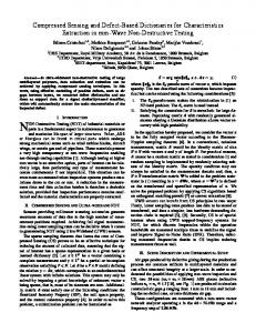
where g1 = s1 , and gi = si − si−1 for i > 1. The gap measure is related to the space needed to represent S in gap encoding [3], which stores the stream of gaps G = g1 , . . . , gn along with the value n instead of S. Note that we cannot merely store each gi in log(gi + 1) bits and decode the stream uniquely; we also need to know the separation boundaries between successive items. One popular technique to “mark” these separators is by using a prefix code such as the δ code [6]. In δ coding, we represent each gi in log(gi + 1) + 2 loglog(gi + 1) bits, where the first loglog(gi + 1) bits are the unary encoding of the number loglog(gi + 1), the next loglog(gi + 1) bits are the binary representation of the number log(gi + 1), and the final log(gi + 1) bits are the binary representation of gi . Given any prefix code, we can uniquely decode the stream G = g1 , g2 , ..., gn by simply concatenating the prefix encoding of each gi . For our theoretical results in this paper, we make use of the δ code. Another example of a prefix code is the nibble code proposed in [4]. In this paper, we will primarily use a variation of the nibble code called nibble4 in our experiments. For this scheme, we write a “nibble” part of log(gi + 1)/4 in unary, which is then followed by 4· log(gi + 1)+ 3/4 bits to write the binary representation of gi , padded out to multiples of four bits. (Later, we describe nibble4fixed, which we use for 64-bit data. It encodes the first part in binary in four bits, since for a universe size of 264 , we would need to write 64/4 = 16 different lengths.) The gap measure is also related to the space needed to represent S in the prefix omission method (POM) described in [10], which is often used to represent bitstrings of arbitrary length. Consider the bitstrings sorted lexicographically. In POM, each bitstring ti is represented with respect to the previous bitstring ti−1 by omitting the common prefix of the two bitstrings. We denote the total length of this stream of (compressed) bits as trie(S). It is shown in [8] that trie(S) ≥ gap(S), and in the worst case, trie(S) is close to 2gap(S); however, if we pick a random number k ∈ U and add it (modulo u) to all the numbers in S (which we call shifting by k), trie(S) is expected to be very close to gap(S). To encode in this amount of space, we need to find a good k. We summarize the relationship between these measures in the following fact.   Fact 1. Both log nu and gap(S)  are smaller than n log u. Also, gap(S)≤ trie(S). When n = o(u), gap(S) ≤ log nu . We provide some experimental results on real data sets in Figure 1, which bears out the theoretical statements of Fact 1. Here, the files tested are described in Section 4.1, and the space is reported (in bits) along the y-axis. The figure on the left shows data files with a universe of size u ≤ 232 , and the figure on the right shows data files with u ≤ 264 .   Notice that gap(S) is significantly smaller than log nu for real data. In fact, nibble4 is a decodeable gap encoding that also outperforms the informationtheoretic minimum. For the IP data files, gap(S) performs relatively poorly,

162

A. Gupta et al.




Fig. 1. Comparison of log nu , trie(S), gap(S), and a gap stream encoded according to the nibble4 code for the data files in Section 4.1

because although IPs tend to be clustered together by domains, within a domain, addresses tend to be more uniformly distributed. On the other hand, the titles file tends to have very tightly-clustered entries, since many books start with the same (or similar) words. As such, this represents a good case for gap encoding. Since gap(S) is less than trie(S) for all of the files, we are free to use gap encoding throughout the remainder of the paper. Also, the impact of gap(S) (and therefore its prefix encodings) is more dramatic for larger universe sizes: the figure on the right showcases this observation for the listed files. In Section 4.2, we show tradeoffs between various prefix codes for both the space required and their encoding/decoding time. It turns out that nibble4 is the method of choice (which is why we included it here).

3

The Binary-Searchable Gap Encoding Scheme (BSGAP)

In this section, we describe our BSGAP data structure that compresses a balanced binary search tree T on S and still supports queries in O(log n) time. The main point of this section is in showing that a binary-searchable representation requires about the same number of bits as linear encoding schemes [10]. (In Section 4.2, we show that this observation also holds in practice.) The basic idea to achieve compression for T is to store each of the n nodes in the binary search tree for S in less than log u bits. In particular, an item s corresponding to node v in the binary search tree will be more succinctly stored if we can store the difference between s and some other item along the path from v to the root. The best such item s would minimize |s − s |. By the properties of binary search trees, s must either be v’s left parent or v’s right parent.1 Generally, let si represent this best ancestor along the path from the root to the node vi corresponding to item si . Formally, let the subsets SL = s1 , s2 , ...sn/2−1  and SR = sn/2+1 , ..., sn  represent the left and right subtrees of the root of the balanced binary search tree 1

The left (right) parent of v is the first node on the path P from v to root that is to the left (right) of v. In a binary search tree, it contains the largest (smallest) item that is smaller (larger) than s among the nodes on P .

Compressed Dictionaries: Space Measures, Data Sets, and Experiments

163

T , which stores the item sn/2 . For the BSGAP of S, denoted as BSGAP(S), let |BSGAP(S)| be the number of bits used to encode BSGAP(S), where we δ-encode each value required. Then, the encoding of BSGAP of S is defined recursively as a concatenation of encoding of four components: BSGAP(S) = sn/2 − sn/2 ; |BSGAP(SL )|; BSGAP(SL ); BSGAP(SR ), where we define sn/2 = 0 to handle encoding the root. The value sn/2 − sn/2 is called the key-value of BSGAP(S). Note the sign of this key-value determines whether the best ancestor is the left parent or the right parent. This value is encoded in variable-length encoding, by the use of a prefix code (such as δ or nibble4) to allow compression. The term |BSGAP(SL )| is needed as a pointer to jump to the the right half of the set while searching, and thus constitutes additional overhead. We shall refer to this space overhead as the pointer cost. In fact, we actually store the encoding of min{|BSGAP(SL )|, |BSGAP(SR )|}, along with an additional bit to indicate which value we have stored. (This improvement saves space both in theory and practice, since the only time one spends any extra bits over the original encoding is when |BSGAP(SL )| = |BSGAP(SR )|.) The search in BSGAP(S) follows exactly the same steps as a search in the original (uncompressed) binary search tree, with the exception that we must decode item values in each node on the fly. In order to maintain an O(log n) query time, we have to consider the issue of decoding a δ-coded number (or similar prefix code) in the RAM model in constant time. We assume that in the RAM model, the word size of the machine is at least log u bits, and that we are allowed to perform addition, subtraction, multiplication, and bitshift operations on words in O(1) time. We also assume that we can calculate the position of the leftmost 1 of a subword x of log log u bits in O(1) time. (This is equivalent to calculating the value log(x + 1) when the word x is seen as an integer.) This latter assumption allows us to decode a δ-coded number (or similar prefix code) in O(1) time in our data structure. If this is not the case, we can simulate the decoding by storing the decoding result of every possible log log u-bit number in a table with log u entries. Note that this table takes O(log u log log log u) bits, which is negligible when compared to the other space terms in our data structure. In summary, we have the following theorem, where the proof is analogous to Lemma 2 in [8], except that we avoid having to find the best shift k that minimizes their space usage. Theorem 1. The BSGAP(S) representation requires gap(S) + O(n log log(u/n)) bits and supports membership, rank and select queries in O(log n) time. Proof. (sketch) Recall that a key-value in the BSGAP structure is storing the difference between an item si and its best ancestor si in the binary search order. Though encoding a particular key-value si −si can take more space than encoding the corresponding gap value gi , we can show that the total space for encoding all the key-values in the BSGAP structure is at most gap(S) + O(n log log(u/n)) bits using a counting technique similar to Lemma 2 of [8]. The remaining space, including the pointer cost and overhead from using δ encoding, can be bounded by O(n log log(u/n)) bits using Jensen’s inequality. 

164

A. Gupta et al.

Now, we describe our main structure, which uses BSGAP as a black box for succinct representation and fast decoding of small blocks. We describe our structure in a bottom-up way. At the bottom level, we group every b items into a block and encode the items in each block by a BSGAP structure. The ith BSGAP structure corresponds to those sj ’s in S with j in [ib + 1, ib + b]. We keep an array P of n/b entries, where P [i] points to the ith BSGAP structure. The array P requires O((n/b) log u) bits of space. At the top level, we collect the first item in each block, and build an instance of Andersson and Thorup’s predecessor structure [1] on these first items, which takes (n/b) log u bits of space. Setting b = log2 n, we achieve the result in the theorem below, which is a slight improvement over Theorem 2 in [8], since we avoid finding a random shift k. As a companion result, we also achieve a worst-case analysis in Corollary 1, since gap(S) and O(n log log(u/n)) are bounded by O(n log(u/n)). Theorem 2. Given a set S of n items from [1, u], we implement a dictionary in gap(S) + O(n log(u/n)/ log n) + O(n log log(u/n)) bits so that rank takes AT (u, n) time and select takes O(log log n) time. Proof. (sketch) To answer select, we only need to traverse one BSGAP structure, thus requiring O(log log n) time. To answer rank, the time is dominated by the predecessor query at the top level, which takes AT (u, n) time. For our space bounds, the n/ log2 n BSGAP data structures require a total of gap(S) + O(n log log(u/n)) bits. The predecessor structure and P take O((n/b) log u) = O(n log(u/n)/ log n) bits of space, thus achieving the stated space bound. 

Corollary 1. We implement a dictionary in at most O(n log(u/n)) bits of space so that rank takes AT (u, n) time and select takes O(log log n) time. In practice, we replace [1] with a simple binary search tree, and introduce a new parameter h = O(log log n) that does not affect the theoretical time for BSGAP but provides a noticeable improvement in practice. Inside each BSGAP-encoded block, we further tune our structure to resort to a simple sequential encoding scheme when there are at most h items left to search, where h < b. Theoretically, the time required to search in the BSGAP structure is still O(log log n). We employ this technique when sequential decoding is fast enough, to save space on the BSGAP pointers used to jump to the right half of the set. In our experiments, we actually let h range up to b, to see the point at which a sequential decoding of h items becomes impractical. It turns out that these few adjustments to our theoretical work result in a fast and succinct practical dictionary.

4

Experimental Results

In this section, we present our experimental results. Section 4.1 describes the experimental setup. In Section 4.2, we discuss various issues with the space requirements of our BSGAP structure and give some intuition about how to encode the various parts of the BSGAP structure efficiently. In Section 4.3, we describe a further tweakable parameter for our BSGAP structure and use it as a black box to succinctly encode blocks of data.

Compressed Dictionaries: Space Measures, Data Sets, and Experiments

165

Apart from the δ code, the nibble code [4], and the nibble4 code we have mentioned in Section 2, in this section, we also refer to a number of variations of prefix codes as follows: – The delta squared code encodes the value log(gi + 1) using δ codes, which is followed by the binary representation of gi . For instance, the delta squared code for 170 is 001 00 1000 10101010. – The nibble4Gamma encodes the “nibble” part of the nibble4 code using γ code instead of unary.2 For instance, the nibble4Gamma code for 170 is 01 0 10101010. – In case the universe size of the data set is at most 232 , we will also have the fixed5 code which encodes the value log(gi + 1) in binary using five bits. For instance, 170 here is encoded as 01000 10101010. – For larger universe sizes (such as our 264 -sized ones), we use the nibble4fixed code, a mix of the nibble4 code and the fixed5 code. Here, we encode the “nibble” part of the nibble4 code using four bits. For each of these codes, we create a small table of values so that we can decode them quickly when appropriate. As described in Section 3, these tables add negligible space, and we have accounted for this (and other) table space in the experimental results that we describe throughout the paper. 4.1

Experimental Setup

Our source code is written in C++ in an object-oriented style. The experiments were run on a Dell PowerEdge 650 with 3 GB of RAM. The machine was running Centos 4.1, with a gnu g++ 3.4.4 compiler. The data sets used were as follows: – IP1: List of IP addresses obtained from Duke University’s Computer Science Department. The list refers to 159,690 IP addresses that hit the Duke CS pages in the month of January 2005. – IP2: Similar to IP1, but this list consists of 148,700 IP addresses that hit the Duke CS pages in February 2005. – UPC 32: List of 100,000 upc codes obtained from items sold by the WalMart supermarket that fit in a universe of size 232 . – ISBN: List of 390,000 ISBNs of books at the Purdue Libraries in a 32-bit format. – UPC 48: List of 432,223 upc codes in the original 48-bit format obtained from items sold by the Wal-Mart supermarket. – Title: List of 256,391 book titles from Purdue Libraries, converted into a numeric value out of a universe of size 264 . 4.2

Code Comparisons for Encodings and Pointers

We performed experiments to compare the space/time tradeoffs of using different encodings in place of nibble4. We summarize those experiments in Figure 2. 2

The “nibble” part will be an integer from [1, 16]. The γ code for an integer x is a unary encoding of log x followed by the binary encoding of x in log(x + 1) bits.

166

A. Gupta et al.

Fig. 2. Comparison of codes and measures for the data files in Section 4.1

The figures in the top row show the time required to process 10,000 randomly generated rank queries with a BSGAP structure using the codes listed, averaged over 10 trials. The figures in the bottom row show the space (in bits) required to encode the BSGAP data structure using the listed prefix codes. Each of the bottom two rows also has the information-theoretic minimum and gap(S) listed for reference. It is clear that both fixed5 and nibble4 are very good codes in the BSGAP structure for the 32-bit case; fixed5 is slightly faster than nibble4, and nibble4 is slightly more space-efficient. (For the ISBN file, nibble4 is significantly more space-efficient.) For 64-bit files, nibble4 is the clear choice. Since our focus is on space efficiency, the rest of the paper will build BSGAP structures with nibble4. (For our 64-bit data sets, we will actually use nibble4fixed.) Next, we investigate the cost of these BSGAP pointers and see if a different choice of code for just the pointers can improve its cost. We summarize the space/time tradeoffs in Figure 3. The figure shows the pointer costs (in bits) of each BSGAP structure. As we can see, nibble4 and nibble are both space-efficient for the pointer distribution. However, nibble4 is again the logical choice, since it is both the most space-efficient and very fast to decode. If we remove these pointer costs from the total space cost for the BSGAP structure, we see that this space is about the same as encoding the gap stream sequentially; as such, we can think of the pointer overhead for BSGAP as a cost to support fast searching.

Compressed Dictionaries: Space Measures, Data Sets, and Experiments

167

Fig. 3. Comparison of prefix codes for BSGAP pointers for the data files in Section 4.1

4.3

BSGAP: The Succinct Binary-Searchable Black Box

In this section, we focus on the practical implementation of our dictionary described in Section 3, which is based on a two-level scheme with a binary search tree at the top and BSGAP structures at the bottom. Recall that there is a parameter b that governs the number of items contained in each BSGAP structure and a parameter h that controls the degree of sequential encoding within a BSGAP data structure. We denote a particular configuration of our dictionary structure by D(b, h). Let BB refer to the data structure in [4]. In this framework, BB is a special case of our dictionary D(b, h) when h = b. In Figure 4, we show a space/time tradeoff for BB and our dictionary. Each graph plots space vs. time, where the time is that required to process 10,000 randomly generated rank queries, averaged over five trials. Here, we tune BB to operate on the same number of items in each block to avoid extra costs for padding and give them the same benefits as BSGAP receives. For each graph in Figure 4, we let the blocksize b range from [2, 256] and the hybrid value range from [2, b]. We collect time and space statistics for each D(b, h) data structure. The BB curve is generated from the 256 points corresponding to D(b, b). For the BSGAP curve, we partition the x-axis into 300 partitions and choose the most time-efficient implementation of D(b, h) taking that much space. Notice that our BSGAP structure converges to BB as we allow more space for the data structures, but we have some improvement for extremely small space. Since BB is a subcase of our BSGAP structure, one might think that our spacetime curve should never be higher than BB’s. However, the curve is generated with actual data structures D(b, h) taking a particular space and time. So, the existence of a point above the BB curve on our BSGAP curve simply means that there exists one configuration of our data structure D(b, h) which has those particular results. The parameter h is crucial to achieving a good space/time tradeoff. Notice that as h increases, the space of D(b, h) decreases because we store fewer pointers in each BSGAP data structure. One may think of transferring this saved space into entries in the top level binary search tree to speed up the query time. On the other hand, the time required to search at the bottom of each BSGAP

168

A. Gupta et al.

Fig. 4. Comparison of BB and BSGAP on 32-bit data files in Section 4.1

Space vs. Time (title)

Time (in sec)

0.0004

BB04 BSGAP

0.0002

0 5000000

8000000

11000000 14000000

Space (in bits)

Fig. 5. Comparison of BB and BSGAP on 48-bit and 64-bit data files in Section 4.1

structure increases linearly with h. So, there must be some moderate value of h that balances these costs and arrives at the best space/time tradeoff. Hence, we collect all (b, h) pairs and evaluate the best candidates among them. In Figure 5, we compare BB and our dictionary for 64-bit data. We plot space vs. time, where the time is that required to process 1,000 randomly generated rank queries, averaged over five trials. We collect data for D(b, h) as before, where the range for b and h for upc 48 is [2, 512] and title is [2, 2048]. Notice that our data structure provides a clear advantage over BB as the universe size increases.

Compressed Dictionaries: Space Measures, Data Sets, and Experiments

5

169

Conclusion

In this paper, we have shown evidence that data-aware measures (such as gap) tend to be smaller than combinatorial measures on real-life data. Employing techniques that exploit the redundancy of the data can lead to more succinct data structures and a better understanding of the underlying information. As such, we encourage researchers to develop theoretical results with a data-aware analysis. In particular, our BSGAP data structure, along with BB (proposed in [4]) are extremely succinct for sparse data sets. In addition, we provide some evidence that BSGAP is less sensitive than [4] to an increase in the size of the universe. Finally, we provide some useful information on the relative performance of prefix codes with respect to compression space and decompression time.

References 1. A. Andersson and M. Thorup. Tight(er) worst-case bounds on dynamic searching and priority queues. In Proceedings of the ACM Symposium on Theory of Computing, 2000. 2. P. Beame and F. Fich. Optimal bounds for the predecessor problem. In Proceedings of the ACM Symposium on Theory of Computing, 1999. 3. T. C. Bell, A. Moffat, C. G. Nevill-Manning, I. H. Witten, and J. Zobel. Data compression in full-text retrieval systems. Journal of the American Society for Information Science, 44(9):508–531, 1993. 4. D. Blandford and G. Blelloch. Compact representations of ordered sets. In Proceedings of the ACM-SIAM Symposium on Discrete Algorithms, 2004. 5. A. Brodnik and I. Munro. Membership in constant time and almost-minimum space. SIAM Journal on Computing, 28(5):1627–1640, 1999. 6. P. Elias. Universal codeword sets and representations of the integers. IEEE Transactions on Information Theory, IT-21:194–203, 1975. 7. R. Grossi and K. Sadakane. Squeezing succinct data structures into entropy bounds. In Proceedings of the ACM-SIAM Symposium on Discrete Algorithms, 2006. 8. A. Gupta, W. Hon, R. Shah, and J. Vitter. Compressed data structures: Dictionaries and data-aware measures. In Proceedings of the IEEE Data Compression Conference, 2006. 9. G. Jacobson. Succinct static data structures. Technical Report CMU-CS-89-112, Carnegie-Mellon University, 1989. 10. S. T. Klein and D. Shapira. Searching in compressed dictionaries. In Proceedings of the IEEE Data Compression Conference, 2002. 11. J. I. Munro. Tables. Foundations of Software Technology and Theoretical Computer Science, 16:37–42, 1996. 12. R. Raman, V. Raman, and S. S. Rao. Succinct indexable dictionaries with applications to encoding k-ary trees and multisets. In Proceedings of the ACM-SIAM Symposium on Discrete Algorithms, pages 233–242, 2002. 13. P. van Emde Boas, R. Kaas, and E. Zijlstra. Design and implementation of an efficient priority queue. Math. Systems Theory, 10:99–127, 1977. 14. D. E. Willard. New trie data structures which support very fast search operations. Journal of Computer and System Sciences, 28(3):379–394, 1984. 15. I. H. Witten, A. Moffat, and T. C. Bell. Managing Gigabytes: Compressing and Indexing Documents and Images. Morgan Kaufmann Publishers, 1999.