Jun 29, 2013 - Normal sensor nodes produce CHs by. Competition. Normal sensor nodes which are not CHs become CMs. .... Electronics and Control. 2011 ...
Sep 19, 2016 - In LTE and LTE-Advance [5], once a transmission is triggered by some ... a random access (RA) procedure by firstly sending a randomly ...
Abstractâ Intelligent Transportation Systems (ITS) often operate on large road networks, and typically collect traffic data with high temporal resolution.
Haar wavelet compression is an efficient way to perform both lossless and lossy
image ... In Matlab, this would be a matrix with unsigned 8-bit integer values. We.
Part II. Image Data Compression. Prof. Ja-Ling Wu. Department of Computer
Science and Information Engineering. National Taiwan University ...
download over a network compared to uncompressed textures, and .... is standardizedâthough not mandatoryâon Android
Jan 30, 2003 ... the general procedure for image compression using wavelets. ... These
theoretical aspects are illustrated through a MATLAB project which.
Nov 28, 2014 - We are grateful to Jimmy Azar and Cris Luengo for helpful discussions. F. Mendivil is partially supported by a grant from the Natural Sciences ...
King's College London (Univ. of London) ... 1st Seminar on Information Technology and its Applications (ITA '91), Markfield Conf. .... H.-O. PEITGEN AND D. SAUPE, The Science of Fractal Image, Springer Verlag, New York, U.S.A., 1988,.
Paul Shelley, Xiaobo Li, Bin Han, âA hybrid quantization scheme for image compressionâ, University of Alberta, 2003. [7]. Martha R. Quispe-Ayala, Krista ...
of the string yz one will detect an occurrence of E(x), which is a wrong match. ... matching scheme for files that were compressed by the LZSS algorithm, and then.
International Journal of Computer Science and Software Engineering (IJCSSE), Volume 5, Issue 11, November 2016. ISSN (Online): 2409-4285 www.IJCSSE.org ... BTC algorithm has good ability to compress an image and the complexity the ...
for high compression rates and non-textured images, this PDE-based approach
gives visually ... The basic idea is to regard the given image data as Dirichlet.
to locate specific landmarks on the face from which Gabor wavelet features are ... each landmark by convolving the image I(x) with the Gabor wavelet of Eq. (1):.
collected during quality evaluations performed on a Dolby. Pulsar HDR monitor. ..... Applications of Digital Image Processing XXXVII, San. Diego, California ...
Mar 9, 2010 - For this type of application, image compression is also the solution. ... agencies, such as the Border Patrol, the Coast Guard, and even the ...
TRANSMISSION RATIO (TR) lossless JPEG. FELICS. LOCO-I. CALIC. SPIHT. SPIHT+arith. Figure 6: SPIHT's performance versus other lossless compressors.
representative codewords to form the codebook. From the .... generate the expanded codebook from the traditional VQ codebook. ..... In VQ, 32.043 dB of image.
Nov 20, 2011 - saved to a different format (.bmp, .tiff). The saved image can be passed to the receiver since the compression rate is unknown. Afterwards, the ...
compression ratio with a higher quality than JPEG. This article describes the digital images compression by compacting energy in the singular values domain.
Received XX Month XXXX; revised XX Month, XXXX; accepted XX Month XXXX; posted XX ..... CALIC) [49] is another extension of CALIC, it modified interband.
packet transform or local trigonometric transform) that yields a table of transform ... The table is called a discrete packet table Ptable with levels l and blocks.
This is done by using a heirarical scalar quantization followed by modified bit- slicing method to select .... (2.11.1) Scalar Quantization⦠..... dr3 dg3 db3. V1. V2.
the field of image coding (the âoldâ JPEG standard has this capabil- ity, as well as ... pdf to fixed size intervals, which have to be predefined before en- coding [16 ...
Compressed Sensing-Based Distributed Image Compression Muhammad Yousuf Baig 1 , Edmund M-K Lai 2, * and Amal Punchihewa 3 1
School of Engineering and Advanced Technology, Massey University, Palmerston North, New Zealand; E-Mail: [email protected] 2 School of Engineering and Advanced Technology, Massey University, Albany, Auckland, New Zealand 3 Asia-Pacific Broadcasting Union, Angkasapuri, Kuala Lumpur 50614, Malaysia; E-Mail: [email protected] * Author to whom correspondence should be addressed; E-Mail: [email protected]; Tel.: +64-9-4140800 Received: 7 October 2013; in revised form: 21 January 2014 / Accepted: 28 February 2014 / Published: 31 March 2014
Abstract: In this paper, a new distributed block-based image compression method based on the principles of compressed sensing (CS) is introduced. The coding and decoding processes are performed entirely in the CS measurement domain. Image blocks are classified into key and non-key blocks and encoded at different rates. The encoder makes use of a new adaptive block classification scheme that is based on the mean square error of the CS measurements between blocks. At the decoder, a simple, but effective, side information generation method is used for the decoding of the non-key blocks. Experimental results show that our coding scheme achieves better results than existing CS-based image coding methods. Keywords: distributed image coding; compressed sensing
1. Introduction Traditional image coding techniques are developed for applications where the source is encoded once and the coded data is played back (decoded) many times. Hence, the encoder is very complex, while the decoder is relatively simple and cheap to implement. However, in many modern applications, such as camera arrays for surveillance, it is desirable to reduced the complexity and cost of the encoder.
Appl. Sci. 2014, 4
129
There are two enabling techniques, which allow reduced complexity encoders to be designed. The first one is distributed coding. Based on the information theoretic work by Wyner and Ziv [1], the coding allows correlated sources to be encoded independently, while the decoder takes advantage of the correlation between source data to improve the quality of the reconstructed images. It has been applied to both image [2,3] and video coding [4]. The second technique is compressed sensing (CS) [5,6]. It has attracted considerable research interest because it allows continuous signals to be sampled at rates much lower than the Nyquist rate for signals that are sparse in some (transform) domain. There have been some application of CS to image coding in the literature. A review is provided in Section 3. Earlier schemes apply CS to the whole image. More recently, block-based coding methods have been proposed [7–10]. The image is divided into non-overlapping blocks of pixels, and each image block is encoded independently. These methods generally use the same measurement rate for all image blocks, even though the compressibility and sparsity of the individual blocks can be quite different. Most proposed coding schemes use a block-based coding approach, where the image is divided into non-overlapping blocks of pixels and each image block is coded independently. They generally use the same measurement rate for all image blocks, even though the compressibility and sparsity of the individual blocks can be quite different [7–10]. For effective and simple CS-based image coding, it is desirable to use a block-based strategy that exploits the statistical structure of the image data. In [11,12], the measurement rate of each block is adapted to the block sparsity. However, it is not easy to estimate the sparsity or compressibility of an image block from the CS measurements alone. In this paper, we take the distributed approach to CS block-based image coding. The image is divided into non-overlapping blocks, and CS measurements for each block are then acquired. Some blocks are designated as key blocks and others as non-key blocks. The non-key blocks are encoded at reduced rates. At the decoder, the reconstruction quality of the non-key blocks is improved by using side information generated from the key blocks. This side information is purely in the CS domain and does not require any prior decoding, making it very simple to generate. We also consider key issues, including the choice of sensing matrix, the measurement (sampling) rate and the reconstruction algorithm. The rest of this paper is organized as follows. Section 2 provides a brief overview of the theory of CS. A review of related works in CS-based image compression is presented in Section 3. Our distributed image coding scheme is presented in Section 4. Section 5 presents experimental results to show the effectiveness of this image codec. 2. Compressed Sensing Shannon’s sampling theorem stipulates that a signal should be sampled at a rate higher than twice the bandwidth of the signal for a successful recovery. For high bandwidth signals, such as image and video, the required sampling rate becomes very high. Fortunately, only a relatively small number of the discrete cosine transform (DCT) or wavelet transform (WT) coefficients of these signals have significant magnitudes. Therefore, coefficients with small magnitudes can be discarded without affecting the quality of the reconstructed signal significantly. This is the basic idea exploited by all existing lossy signal compression techniques. The idea of CS is to acquire (sense) these significant information directly
Appl. Sci. 2014, 4
130
without first sampling the signal in the traditional sense. It has been shown that if the signal is “sparse” or compressible, then the acquired information is sufficient to reconstruct the original signal with a high probability [5,6]. Sparsity is defined with respect to an appropriate basis, such as DCT or WT, for that signal. The theory also stipulates that the CS measurements of the signal must be acquired through a process that is incoherent with the signal. Incoherence makes certain that the information acquired is randomly spread out in the basis concerned. In CS, the ability of a sensing technique to effectively retain the features of the underlying signal is very important. The sensing strategy should provide a sufficient number of CS measurements in a non-adaptive manner that enables near perfect reconstruction. Let f = {f1 , . . . , fN } be N real-valued samples of a signal, which can be represented by the transform coefficients, x. That is, N X f = Ψx = xi ψi (1) i=1
where Ψ = [ψ1 , ψ2 . . . ψN ] is the transform basis matrix and x = [x1 , . . . , xN ] is an N -vector of coefficients with xi =< x, ψi >. We assume that x is S-sparse, meaning that there are only S 0.9). This means that we can make use of this correlation for distributed coding of CS measurements. Furthermore, the MSE values of the image data are reflected in those of the CS measurement. Hence, we can use the MSE of the CS measurements as an indication of the MSE of the original image data. Thus, similar image blocks have low MSE values of CS measurements. To evaluate the effect of block size on image block similarity, the percentage of correlated blocks exceeding an MSE threshold is computed for block sizes of 64 × 64, 32 × 32, 16 × 16 and 8 × 8. Figure 1 shows the results for the four images. As expected, there are more correlated blocks for smaller block sizes. Blocks with a size of 64 × 64 can virtually be considered independent. The percentage of blocks that can be considered correlated depends on the MSE threshold. Thus, a smaller block size with appropriate MSE threshold would be desirable for our codec. Figure 1. Percentage of similar blocks for the block size (64, 32, 16 and eight) for (a) Lena; (b) Boat; (c) Cameraman; and (d) Goldhill. 70
4.2. The Encoder A block diagram of the proposed encoder is shown in Figure 2a. At the encoder, an image with a dimension of N × N pixels is divided into B non-overlapping blocks of NB × NB pixels. Let xi represent the i-th block with CS measurements yi = ΦB xi . Each image block is classified either as a key block or a non-key (WZ) block. They are encoded using CS measurement rates of Mk and Mw respectively, where Mk Mw . The CS measurements are then quantized using the quantization scheme proposed in our earlier work [39]. Figure 2. Proposed distributed intra-image codec: (a) the encoder and (b) the decoder. CS, compressed sensing.
Key Blocks
Adaptive Encoding
Initial CS Measurements
CS Encoding
Estimating Similarity Non-Key (WZ) Blocks
Image
Quantization
Quantization
Block Division
Non-Adaptive Encoding
(a)
Key Blocks
CS Encoding
Quantization
Non-Key (WZ) Blocks
CS Encoding
Quantization
Appl. Sci. 2014, 4
136 Figure 2. Cont.
Key Block Decoding Inverse Quantization
CS Decoding
Dictionary
Inverse Quantization
Decoded Key Blocks
Side Information Generation
CS Decoding
WZ Block Decoding
Decoded WZ Blocks
(b) The way by which the image blocks are classified affects the compression ratio, as well as the quality of the reconstructed image. The number of CS measurements required to reconstruct a signal is dependent on the sparsity of the signal. If a block has high sparsity, then it can be reconstructed with fewer measurements compared with a block with low sparsity. If a low sparsity block is encoded with a low measurement rate, the reconstruction quality will be poor. Determining the sparsity of an image block is a challenging problem. Two different block classification schemes, one non-adaptive and the other adaptive, are proposed here. 4.2.1. Non-Adaptive Block Classification The non-adaptive block classification scheme is designed for very low complexity encoding with minimum computation. In this scheme, the blocks are classified sequentially according to the order position in which they are acquired. A group of consecutive M blocks is referred to as a group of blocks (GOB). The first block in a GOB is a key block. The remaining M − 1 blocks are WZ blocks. Block sparsity is not considered in this scheme. It is similar to the concept of group of picture (GOP) used in traditional video coding. If M = 1, then every block is a key block and is encoded at the same rate. The average measurement rate decreases as M increases. 4.2.2. Adaptive Block Classification The adaptive block classification scheme can be deployed for encoders with more computing resources. This scheme requires the creation of a dictionary of CS measurements of key blocks. This
Appl. Sci. 2014, 4
137
dictionary is initially empty. The first block of the image is always a key block. The CS measurements of this block become the first entry of the dictionary. For each subsequent image block, the MSE between its CS measurements and the entries in the dictionary is computed. If any of these MSEs computed falls below a threshold, λ, then this block is classified as a WZ block and will be encoded at the lower rate. Otherwise, it is a key block, and its measurements are added to the dictionary as a new entry. In order to reduce the resources required, the size of the dictionary can be limited. When the dictionary is full and a new entry is needed, the oldest entry will be discarded. The threshold, λ, is determined adaptively as follows. For each image block, i, the threshold is obtained by: λ = C · median(|yi |) (10) where yi are the CS measurements of block i and C is a constant. The value of C controls the relative number of key blocks and WZ blocks. If C > 1, the number of WZ blocks will be increased. Choosing C < 1 will increase the number of key blocks. This method reduces the encoding delay compared with SD-based methods described in Section 3. The entire encoding process is summarized in Algorithm 1. Algorithm 1 Adaptive CS encoding. Input:yw , D for each column i inD do Calculate r[i] = M SE(yw , D) end for Calculate τ = min[r] Estimate λ = C.median(|yw |) if τ > λ then yk (key block) else if τ < λ then yw (WZ block) end if end if
4.3. The Decoder The decoder has to reconstruct the full image from the CS measurements of the individual image blocks. A block diagram of the proposed decoder is shown in Figure 2b. The key issue that affects the quality of the reconstructed image is the CS reconstruction strategy. This will be discussed in Section 4.3.1. The theory of distributed coding tells us that side information is needed to reconstruct these blocks effectively. So, for a distributed codec, another issue to be addressed is the generation of appropriate side information. This will be addressed in Section 4.3.2.
Appl. Sci. 2014, 4
138
Figure 3. Block-based CS reconstruction comparison: (a) The original image; (b) independent block recovery; and (c) joint recovery. PSNR, peak signal-to-noise ratio.
(a) Lena Original
(b) Lena Independent PSNR = 28.04 dB
(c) Lena Joint, PSNR = 28.23 dB
4.3.1. Reconstruction Approach There are three approaches by which the full image can be recovered from the block-based CS measurements. The first one is to reconstruct each block from its CS measurements independently of the other blocks, using the corresponding sensing and block sparsifying matrices. This is the independent block recovery approach. The second way is to place a block sparsifying transform in to a block diagonal sparsifying matrix and then use the block diagonal sparsifying transform to reconstruct the full image [40]. In this approach, instead of reconstructing independent blocks, CS measurements of all the blocks are used to reconstruct the full image. The reconstruction performances of these two
Appl. Sci. 2014, 4
139
approaches are almost the same [40]. Alternatively, all image blocks can be reconstructed jointly using a full sparsifying matrix [40]. This approach is known as joint recovery. Instead of using the block sparsifying matrix or the block diagonal sparsifying matrix, a full sparsifying transform is applied to the CS measurements of all sampled blocks combined to reconstruct the full image. This is better than independent and diagonal reconstruction, as a full transform promotes a sparser representation and blocking artefacts can be avoided, as well. Generally speaking, the difference in the peak signal-to-noise ratio (PSNR) between independent and joint recovery is not significant. However, blocking artefacts can be an issue for independently recovered images, as shown in Figure 3. Based on this knowledge, the strategy adopted for our decoder is as follows. Each individual image block is recovered as they become available at the decoder. This is used as an initial solution. Once all the blocks are available at the decoder, a joint reconstruction is performed to provide a visually better result. 4.3.2. Side Information Generation At the decoder, after inverse quantization, the key blocks are reconstructed from their own CS measurements. For WZ blocks, reconstruction is performed with the help of side information, which is generated through a dictionary. Since the CS measurements of adjacent image blocks are highly correlated, those of the key blocks can be used directly as side information (SI). Starting with an empty dictionary, D, it is populated with the (inverse quantized) CS measurements of the key blocks as they are received. With non-adaptive block classification, each key block is followed by one or more WZ blocks. For the WZ blocks in the same GOB, D has only one entry: D1 . Therefore, D1 is used as the SI to reconstruct this WZ block. For the WZ blocks in the next GOB, the dictionary will have two entries from the two key blocks received so far. The entry in the dictionary that is chosen as SI is the one that has the minimum MSE with the current WZ block. This process continues, until all the WZ blocks are reconstructed. With adaptive block classification, the WZ blocks are reconstructed in a similar way. The only difference is that the number of WZ blocks following each key block is not fixed. There are several advantages with this SI generation method. Firstly, it does not require the key blocks to be decoded first. Secondly, the dictionary only consists of CS measurements of key blocks, which are already available for decoding. Therefore, it does not need to be computed or learned. Most importantly, SI obtained in this way can be directly used by the CS reconstruction algorithm without any further processing. 5. Experimental Results Twelve standard test images [41] are used to evaluate the effectiveness of the proposed distributed CS image codec. They are shown in Figure 4. These images are 512 × 512 pixels in size and contain different content and textures. The visual reconstruction quality of the reconstructed images is evaluated by the peak signal-to-noise ratio (PSNR) and the structural similarity index (SSIM). The compression efficiency of the codec is evaluated by bits per pixel (bpp). The average measurement rate is the average including both the key and WZ blocks.
Appl. Sci. 2014, 4
140
Figure 4. Standard test images with their corresponding titles used in the experiments.
(a) Lenna
(b) Boat
(c) Camerman
(d) Goldhill
(e) Barbara
(f) Clown
(g) Crowd
(h) Couple
(i) Girl
(j) Man
(k) Mandrill
(l) Peppers
In Section 4.1, it has been shown that smaller block sizes yield a larger percentage of correlated blocks. Therefore, in these experiments, a block size of 8×8 pixels is used. A scrambled block Hadamard ensemble (SBHE) sensing matrix is used to obtain the CS measurements, and Daubechies 9/7 wavelets are used as the sparsifying matrix. The SpaRSA [24] algorithm is used as the reconstruction algorithm at the decoder. The proposed adaptive and non-adaptive approach with and without SI at the decoder is compared with two other techniques. The first one is the encoding of image blocks with the same measurement rate, i.e., no distinction of the key and WZ blocks. It is labelled as “Fixed Rate” in the results. The second technique is first proposed in [12] and recently used to classify image blocks as compressible or incompressible [11]. It is labelled as the “SD approach” in the results. The idea is that if the SD of the CS measurements of an image block is higher than the SD of the full image, then the block is classified as incompressible, and more measurements are required for successful reconstruction. The authors of [12] used the original image data to compute the SD, which is not possible in real-world applications. For the adaptive block selection, C = 1 is used. All codecs are coded in MATLAB R2012b and simulations run on an Intel i5 3.6 GHz, Windows 7 Enterprise Edition, 64-bit Operating
Appl. Sci. 2014, 4
141
System with 4 GB of RAM. For each measurement rate per image, the experiment is run five times, and then, the average is reported.
32
30
31
29
30
28
29
27 PSNR (dB)
PSNR (dB)
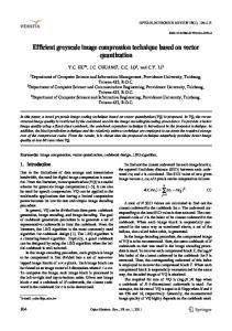
Figure 5. Rate-distortion performance for the test images: (a) Lena; (b) Boat; (c) Cameraman; and (d) Couple.
28 27 26
25 24
STD Approach Adaptive(Proposed, No SI) Adaptive(Proposed, With SI) Non−Adaptive(Proposed, No SI) Non−Adaptive(Proposed, with SI) Fixed Rate
25 24 23
26
0.2
0.25
0.3 0.35 0.4 Average Measurement Rate (%)
0.45
0.5
STD Approach Adaptive(Proposed, No SI) Adaptive(Proposed, With SI) Non−Adaptive(Proposed, No SI) Non−Adaptive(Proposed, with SI) Fixed Rate
23 22 21
0.55
0.2
0.25
(a)
0.3 0.35 0.4 Average Measurement Rate (%)
0.45
0.5
0.55
(b)
34
29 28
32 27 26 PSNR (dB)
PSNR (dB)
30
28
26
24 23
STD Approach Adaptive(Proposed, No SI) Adaptive(Proposed, With SI) Non−Adaptive(Proposed, No SI) Non−Adaptive(Proposed, with SI) Fixed Rate
24
22
25
0.2
0.25
0.3 0.35 0.4 Average Measurement Rate (%)
(c)
0.45
0.5
0.55
STD Approach Adaptive(Proposed, No SI) Adaptive(Proposed, With SI) Non−Adaptive(Proposed, No SI) Non−Adaptive(Proposed, with SI) Fixed Rate
22 21 20
0.2
0.25
0.3 0.35 0.4 Average Measurement Rate (%)
0.45
0.5
0.55
(d)
Figure 5 shows the R-D curves for four test images (“Lenna”, ”Boat”, “Cameraman” and “Couple”). The proposed adaptive sensing scheme with and without SI at the decoder outperforms all other algorithms for all test images. The non-adaptive scheme without SI is comparable with “Fixed Rate” and “SD Approach”. The non-adaptive scheme with SI improves the reconstruction quality and produces better results than “Fixed Rate” and “SD Approach”. The visual reconstruction quality evaluation for the above four images on the basis of structure similarity index [42] is shown in Figure 6. The visual
Appl. Sci. 2014, 4
142
quality of the adaptive scheme and the non-adaptive scheme with SI is superior for all test images. Table 1 shows the R-D performance of all twelve images averaged for all measurement rates. Again, the adaptive scheme outperforms all other schemes. The lowest average MR is obtained for “Cameraman”, “Girl” and “Lena” with the adaptive scheme; the PSNR is more than 1.5 dB better than other schemes. However, for an image with less intra-image similarity, like “Mandrill”, the adaptive scheme requires a higher number of measurements than other approaches. Using the proposed SI generation method improves reconstruction performance for both adaptive and non-adaptive encoding.
0.94
0.92
0.92
0.89
0.9
0.86
0.88
0.83 SSIM Index
SSIM Index
Figure 6. SSIM Index for Test Images, (a) Lena; (b) Boat; (c) Cameraman and (d) Couple.
0.86 0.84 0.82
0.77 0.74
STD Approach Adaptive(Proposed, No SI) Adaptive(Proposed, With SI) Non−Adaptive(Proposed, No SI) Non−Adaptive(Proposed, with SI) Fixed Rate
0.8 0.78 0.76
0.8
0.2
0.25
0.3 0.35 0.4 Average Measurement Rate (%)
0.45
0.5
STD Approach Adaptive(Proposed, No SI) Adaptive(Proposed, With SI) Non−Adaptive(Proposed, No SI) Non−Adaptive(Proposed, with SI) Fixed Rate
0.71 0.68 0.65
0.55
0.2
0.25
(a)
0.3 0.35 0.4 Average Measurement Rate (%)
0.45
0.5
0.55
(b)
0.94
0.9
0.92
0.87
0.9
0.84
0.88
0.81 SSIM Index
SSIM Index
0.96
0.86 0.84
0.78 0.75 0.72
0.82
STD Approach Adaptive(Proposed, No SI) Adaptive(Proposed, With SI) Non−Adaptive(Proposed, No SI) Non−Adaptive(Proposed, with SI) Fixed Rate
0.8 0.78
STD Approach Adaptive(Proposed, No SI) Adaptive(Proposed, With SI) Non−Adaptive(Proposed, No SI) Non−Adaptive(Proposed, with SI) Fixed Rate
0.69 0.66 0.63
0.76
0.2
0.25
0.3 0.35 0.4 Average Measurement Rate (%)
(c)
0.45
0.5
0.55
0.2
0.25
0.3 0.35 0.4 Average Measurement Rate (%)
(d)
0.45
0.5
0.55
Appl. Sci. 2014, 4
143
Table 1. Performance evaluation using the test images according to measurement rate (MR), pixel signal-to-noise ration (PSNR), and structural similarity index(SSIM).
Image
Criteria
SD Approach
Fixed Rate
Non-Adaptive (No SI)
Non-Adaptive (SI)
Adaptive (No SI)
Adaptive (SI)
Boat
MR PSNR SSIM
38% 24.87 0.81
35% 25.36 0.82
35% 25.14 0.81
35% 25.60 0.83
35% 26.27 0.83
35% 26.62 0.84
Barbara
MR PSNR SSIM
35% 23.95 0.81
35% 23.57 0.81
35% 23.62 0.81
35% 24.05 0.83
37% 24.64 0.84
37% 24.89 0.85
Camera man
MR PSNR SSIM
38% 27.02 0.87
35% 27.18 0.88
35% 26.78 0.87
35% 27.55 0.89
31% 28.74 0.89
31% 29.21 0.90
Couple
MR PSNR SSIM
36% 24.99 0.80
35% 25.11 0.81
35% 24.82 0.80
35% 25.40 0.82
36% 26.19 0.83
36% 26.58 0.84
Clown
MR PSNR SSIM
33% 26.84 0.82
35% 26.01 0.84
35% 26.06 0.85
35% 26.89 0.87
37% 26.66 0.86
37% 28.09 0.89
Crowd
MR PSNR SSIM
32% 25.83 0.84
35% 25.00 0.85
35% 24.51 0.84
35% 25.24 0.86
37% 26.20 0.88
37% 26.79 0.89
Girl
MR PSNR SSIM
37% 27.76 0.83
35% 28.45 0.82
35% 28.04 0.82
35% 28.73 0.84
31% 28.55 0.82
31% 29.20 0.83
Goldhill
MR PSNR SSIM
34% 26.68 0.79
35% 27.01 0.81
35% 26.76 0.81
35% 27.07 0.82
37% 26.53 0.82
37% 27.89 0.84
Lena
MR PSNR SSIM
36% 27.14 0.86
35% 27.56 0.87
35% 27.55 0.87
35% 27.96 0.88
32% 28.30 0.88
32% 28.88 0.89
Man
MR PSNR SSIM
36% 25.84 0.81
35% 25.98 0.82
35% 25.59 0.81
35% 26.00 0.82
36% 26.70 0.84
36% 27.26 0.85
Mandrill
MR PSNR SSIM
35% 21.01 0.68
35% 21.07 0.68
35% 21.10 0.69
35% 21.12 0.69
41% 21.96 0.75
41% 22.18 0.75
Peppers
MR PSNR SSIM
33% 26.83 0.88
35% 26.45 0.87
35% 26.60 0.88
35% 27.48 0.90
33% 27.59 0.89
33% 28.29 0.90
Appl. Sci. 2014, 4
144
32
30
31
29
30
28
29
27 PSNR (dB)
PSNR (dB)
Figure 7. Compression efficiency for the test images: (a) Lena; (b) Boat; (c) Cameraman; and (d) Couple.
28 27 26
25 24
25
23
STD Approach Adaptive(Proposed, No SI) Adaptive(Proposed, With SI) Fixed Rate
24 23 0.05
26
0.1
0.15
0.2 0.25 Bitrate (bpp)
0.3
0.35
STD Approach Adaptive(Proposed, No SI) Adaptive(Proposed, With SI) Fixed Rate
22 21 0.05
0.4
0.1
0.15
(a)
0.2 0.25 Bitrate (bpp)
0.3
0.35
0.4
(b)
33
29
32
28
31 27
26
29
PSNR (dB)
PSNR (dB)
30
28 27
25
24
26 23 25
STD Approach Adaptive(Proposed, No SI) Adaptive(Proposed, With SI) Fixed Rate
24 23 0.05
0.1
0.15
0.2 0.25 Bitrate (bpp)
(c)
0.3
0.35
0.4
STD Approach Adaptive(Proposed, No SI) Adaptive(Proposed, With SI) Fixed Rate
22
21 0.05
0.1
0.15
0.2 0.25 Bitrate (bpp)
0.3
0.35
0.4
(d)
To evaluate the compression efficiency of the proposed distributed image codec, the CS measurements are quantized using the quantization scheme proposed in [39]. Each CS measurement is allotted eight bits for quantization. The quantized CS measurements are then entropy coded using Huffman coding. Figure 7 shows the PSNR performance of four test images at different bit rates. The compression efficiency of the adaptive scheme with SI is higher than the “Fixed Rate” and “SD” schemes at the same reconstruction quality. At lower average measurement rates, the “Fixed Rate” scheme performs better than the adaptive scheme with no SI for images “Boat” and “Couple”.
Appl. Sci. 2014, 4
145
6. Conclusions In this article, a new distributed block-based CS image codec has been proposed. The coding is performed entirely in the CS measurement domain. It has two special features. The first one is the way by which image blocks are classified as key or non-key. The adaptive classification method proposed is based on the experimental analysis of the MSE of the CS measurements between image blocks. At the decoder, the CS measurements of the key blocks are used as side information for the decoding of non-key blocks. The choice of which measurements are used is again based on the MSE of CS measurements. This SI generation technique is simple to implement, yet very effective in improving the reconstruction quality of WZ blocks. It can also be easily integrated with any CS reconstruction algorithm without the need for modification. Experimental data show that this codec outperforms “Fixed Rate” and SD-based approaches for all the test images. Conflicts of Interest The authors declare no conflict of interest. References 1. Wyner, A. Recent Results in the Shannon Theory. IEEE Trans. Inf. Theory 1974, 20, 2–10. 2. Dikici, C.; Guermazi, R.; Idrissi, K.; Baskurt, A. Distributed source coding of still images. In Proceedings of 13th European Signal Processing Conference, Antalya, Turkey, 4–8 September 2005. 3. Zhang, J.; Li, H.; Chen, C.W. Distributed image coding based on integrated markov modeling and LDPC decoding. In Proceedings of IEEE International Conference on Multimedia and Expo, Hannover, Germany, 23–26 June 2008; pp. 637–640. 4. Girod, B.; Aaron, A.; Rane, S.; Rebollo-Monedero, D. Distributed Video Coding. IEEE Proc. 2005, 93, 71–83. 5. Donoho, D. Compressed Sensing. IEEE Trans. Inf. Theory 2006, 52, 1289–1306. 6. Candes, E.; Romberg, J.; Tao, T. Robust Uncertainty Principles: Exact Signal Reconstruction from Highly Incomplete Frequency Information. IEEE Trans. Inf. Theory 2006, 52, 489–509. 7. Gan, L. Block compressed sensing of natural images. In Proceedings of 15th International Conference on Digital Signal Processing, Cardiff, Wales, 1–4 July 2007; pp. 403–406. 8. Mun, S.; Fowler, J.E. Block compressed sensing of images using directional transforms. In Proceedings of 16th IEEE International Conference on Image Processing, Cairo, Egypt, 7–12 November 2009; pp. 3021–3024. 9. Yang, Y.; Au, O.; Fang, L.; Wen, X.; Tang, W. Perceptual compressive sensing for image signals. In Proceedings of IEEE International Conference on Multimedia and Expo, Cancun, Mexico, 28 June–3 July 2009; pp. 89–92. 10. Gao, Z.; Xiong, C.; Zhou, C.; Wang, H. Compressive sampling with coefficients random permutations for image compression. In Proceedings of the International Conference on Multimedia and Signal Processing, Guilin, China, 14–15 May 2011; Volume 1, pp. 321–324.
Appl. Sci. 2014, 4
146
11. Zhang, X.; Chen, J.; Meng, H.; Tian, X. Self-adaptive Structured Image Sensing. Opt. Eng. 2012, 51, 127001:1–127001:3. 12. Sun, L.; Wen, X.; Lei, M.; Xu, H.; Zhu, J.; Wei, Y. Signal Reconstruction Based on Block Compressed Sensing. In Artificial Intelligence and Computational Intelligence; Springer: Berlin, Germany, 2011; Volume 7003, pp. 312–319. 13. Baraniuk, R. Compressive Sensing [Lecture Notes]. IEEE Signal Process. Mag. 2007, 24, 118–121. 14. Candes, E.; Wakin, M. An Introduction to Compressive Sampling. IEEE Signal Process. Mag. 2008, 25, 21–30. 15. Chen, S.; Donoho, D. Basis pursuit. In Proceedings of IEEE Asilomar Conference on Signals, Systems and Computers, Pacific Grove, CA, USA, November 1994; Volume 1, pp. 41–44. 16. Chen, S.; Donoho, D.; Saunders, M. Atomic Decomposition by Basis Pursuit. SIAM Rev. 2001, 43, 129–159. 17. Tibshirani, R. Regression Shrinkage and Selection via the Lasso. J. R. Stat. Soc. Ser. B 1994, 58, 267–288. 18. Mallat, S.; Zhang, Z. Matching Pursuit with Time-Frequency Dictionaries. IEEE Trans. Signal Process. 1993, 41, 3397–3415. 19. Tropp, J.; Gilbert, A. Signal Recovery From Partial Information via Orthogonal Matching Pursuit. IEEE Trans. Inf. Theory 2007, 53, 4655–4666. 20. Donoho, D.; Tsaig, Y.; Drori, I.; Starck, J.L. Sparse Solution of Underdetermined Systems of Linear Equations by Stagewise Orthogonal Matching Pursuit. IEEE Trans. Inf. Theory 2012, 58, 1094–1121. 21. Needell, D.; Tropp, J. CoSaMP: Iterative Signal Recovery From Incomplete and Inaccurate Samples. Appl. Comput. Harmon. Anal. 2009, 26, 301 – 321. 22. Figueiredo, M.; Nowak, R.; Wright, S. Gradient Projection for Sparse Reconstruction: Application to Compressed Sensing and other Inverse Problems. IEEE J. Sel. Topics Signal Process. 2007, 1, 586–597. 23. van den Berg, E.; Friedlander, M.P. Probing the Pareto Frontier for Basis Pursuit Solutions. SIAM J. Sci. Comput. 2008, 31, 890–912. 24. Wright, S.J.; Nowak, R.D.; Figueiredo, M.A.T. Sparse Reconstruction by Separable Approximation. IEEE Trans. Signal Process. 2009, 57, 2479–2493. 25. Bioucas-Dias, J.M.; Figueiredo, M.A.T. A New TwIST: Two-Step Iterative Shrinkage/Thresholding Algorithms for Image Restoration. IEEE Trans. Image Process. 2007, 16, 2992–3004. 26. Candes, E.J.; Romberg, J. Practical signal recovery from random projections. In Proceedings of SPIE Computational Imaging, San Jose, CA, USA, January 2005; Volume 5674, pp. 76–86. 27. Do, T.; Nguyen, L.G.N.; Tran, T.D. Sparsity adaptive matching pursuit algorithm for practical compressed sensing. In Proceedings of 42nd IEEE Asilomar Conference on Signals, Systems and Computers, Pacific Grove, CA, USA, 26–29 October 2008. 28. Do, T.; Gan, L.; Tran, T. Fast compressive sampling with structurally random matrices. In Proceedings of IEEE International Conference on Acoustics, Speech and Signal Processing, Las Vegas, NV, USA, 30 March–4 April 2008; pp. 3369–3372.
Appl. Sci. 2014, 4
147
29. Lu Gan, T.D.; Tran, T. Fast Compressive Imaging Using Scrambled Block Hadamard Ensemble. In Proceedings of European Signal Processing Conference, Lausanne, Switzerland, 25–29 August 2008. 30. Tsaig, Y.; Donoho, D.L. Extensions of Compressed Sensing. Signal Process. 2006, 86, 549–571. 31. Han, B.; Wu, F.; Tian, X. Image Representation by Compressive Sensing for Visual Sensor Networks. J. Vis. Commun. Image Represent. 2010, 21, 325–333. 32. J. E. Fowler, S.M.; Tramel, E.W. Multiscale block compressed sensing with smoothed projected landweber Reconstruction. In Proceedings of European Signal Processing Conference, Barcelona, Spain, 29 August–2 September 2011; pp. 564–568. 33. Ji, S.; Xue, Y.; Carin, L. Bayesian Compressive Sensing. IEEE Trans. Signal Process. 2008, 56, 2346–2356. 34. He, L.; Carin, L. Exploiting Structure in Wavelet-Based Bayesian Compressive Sensing. IEEE Trans. Signal Process. 2009, 57, 3488–3497. 35. He, L.; Chen, H.; Carin, L. Tree-Structured Compressive Sensing With Variational Bayesian Analysis. IEEE Signal Process. Lett. 2010, 17, 233–236. 36. Babacan, S.; Molina, R.; Katsaggelos, A. Bayesian Compressive Sensing Using Laplace Priors. IEEE Trans. Image Process. 2010, 19, 53–63. 37. Xie, S.; Rahardja, S.; Li, Z. Wyner-Ziv image coding from random projections. In Proceedings of IEEE International Conference on Multimedia and Expo, Beijing, China, 2–5 July 2007; pp. 136–139. 38. Gan, Z.; Qi, L.; Zhu, X. Wyner-Ziv coding of image using compressed sensing. In Proceedings of International Symposium on Intelligent Signal Processing and Communication Systems, Chengdu, China, 6–8 December 2010; pp. 1–4. 39. Baig, Y.; Lai, E.; Lewis, J. Quantization effects on compressed sensing video. In Proceedings of 17th International Telecommunications Conference, Doha, Qatar, 4–7 April 2010; pp. 917–922. 40. Fowler, J.E.; Mun, S.; Tramel, E.W. Block-Based Compressed Sensing of Images and Video. Found. Trends Signal Process. 2012, 4, 297–416. 41. Test Images. Available online: http://decsai.ugr.es/cvg/dbimagenes/index.php (accessed on 20 March 2014). 42. Wang, Z.; Bovik, A.C.; Sheikh, H.R.; Simoncelli, E.P. Image Quality Assessment: From Error Visibility to Structural Similarity. IEEE Trans. Image Process. 2004, 13, 600–612. c 2014 by the authors; licensee MDPI, Basel, Switzerland. This article is an open access article
distributed under the terms and conditions of the Creative Commons Attribution license (http://creativecommons.org/licenses/by/3.0/).