Jan 24, 2014 - CSâfMRI with GRE, but not with EPI, improves the statistical sensitivity for. 24 ..... sists of electri
YNIMG-11124; No. of pages: 10; 4C: 4, 6, 7, 8 NeuroImage xxx (2014) xxx–xxx
Contents lists available at ScienceDirect
NeuroImage journal homepage: www.elsevier.com/locate/ynimg
F
Q1
Compressed sensing fMRI using gradient-recalled echo and EPI sequences Xiaopeng Zong a,e,1, Juyoung Lee b,1, Alexander Poplawsky a, Seong-Gi Kim a,c,d, Jong Chul Ye b,⁎
O
1
a
Neuroimaging Laboratory, Department of Radiology, University of Pittsburgh, Pittsburgh, PA 15203, USA Bio-Imaging & Signal Processing Lab., Korea Advanced Institute of Science & Technology (KAIST), 373-1 Guseong-Dong, Yuseong-Gu, Daejon 305-701, Republic of Korea Center for Neuroscience Imaging Research, Institute for Basic Science (IBS), Daejeon 305-701, Republic of Korea d Department of Biological Science, Sungkyunkwan University, Suwon 440-746, Republic of Korea e Biomedical Research Imaging Center, University of North Carolina at Chapel Hill, Chapel Hill, NC 27599, USA b
18 6 19 7 20 8 21 9 22 10 23 11 12 24 13 25 14 26
Keywords: Compressed sensing fMRI k–t FOCUSS Olfactory bulb Somatosensory cortex BOLD CBV High magnetic field
Compressed sensing (CS) may be useful for accelerating data acquisitions in high-resolution fMRI. However, due to the inherent slow temporal dynamics of the hemodynamic signals and concerns of potential statistical power loss, the CS approach for fMRI (CS–fMRI) has not been extensively investigated. To evaluate the utility of CS in fMRI application, we systematically investigated the properties of CS–fMRI using computer simulations and in vivo experiments of rat forepaw sensory and odor stimulations with gradient-recalled echo (GRE) and echo planar imaging (EPI) sequences. Various undersampling patterns along the phase-encoding direction were studied and k–t FOCUSS was used as the CS reconstruction algorithm, which exploits the temporal redundancy of images. Functional sensitivity, specificity, and time courses were compared between fully-sampled and CS–fMRI with reduction factors of 2 and 4. CS–fMRI with GRE, but not with EPI, improves the statistical sensitivity for activation detection over the fully sampled data when the ratio of the fMRI signal change to noise is low. CS improves the temporal resolution and temporal noise correlations. While CS reduces the functional response amplitudes, the noise variance is also reduced to make the overall activation detection more sensitive. Consequently, CS is a valuable fMRI acceleration approach, especially for GRE fMRI studies. © 2014 Published by Elsevier Inc.
D
Article history: Accepted 24 January 2014 Available online xxxx
E
3 15 4 16 5 17
a b s t r a c t
P
i n f o
T
a r t i c l e
C
2
R O
c
E
27 28 32 30 29
R
31
Introduction
34
Compressed sensing (CS) theory (Candes et al., 2006; Donoho, 2006) has been gathering interest in the MR community due to its potential for accelerated image acquisition without compromising image quality. Specifically, CS theory informs us that an accurate reconstruction from undersampled measurements below the Nyquist sampling limit is possible using a nonlinear reconstruction algorithm if the image is sparse in some transform domain and the sensing matrix is sufficiently incoherent. In many dynamic imaging applications, such as cardiac cine MRI, various compressed sensing algorithms have been successfully implemented by exploiting the temporal redundancies of images (Feng et al., 2011; Hu et al., 2012; Jung and Ye, 2010; Jung et al., 2007, 2009, 2010; Lingala et al., 2011; Lustig et al., 2006; Usman et al., 2011; Zhao et al., 2010). A similar CS approach is potentially useful for high-resolution fMRI to improve the temporal resolution since such temporal redundancies exist in fMRI data (Jung and Ye, 2009; Lu and Vaswani, 2011; Nguyen and Glover, 2013).
39 40 41 42 43 44 45 46 47 48 49
N C O
37 38
U
35 36
R
33
⁎ Corresponding author at: Bio-Imaging & Signal Processing Lab., Korea Advanced Institute of Science & Technology (KAIST), 373-1 Guseong-Dong, Yuseong-Gu, Daejon 305-701, Republic of Korea. 1 Contribute equally.
In fMRI studies with a relatively low spatial resolution (e.g. ~3 × 3 × 3 mm3 in human brain at 3 T), whole brain images can be acquired by the single-shot echo planar imaging technique within 2 s. Given the inherently slow hemodynamic responses, the CS approach may not be necessary for routine low resolution human fMRI studies, but may be useful for studies requiring long image repetition times. One example is to acquire high-resolution fMRI with multi-shot EPI sequences, which increase the repetition time (TR) by a factor equal to the additional number of shots. Another obvious case is conventional gradientrecalled echo (GRE) fMRI studies (Frahm et al., 1993; Kida et al., 2002; Ogawa et al., 1992). The GRE approach is often used for imaging highly field-inhomogeneous regions, especially in small animals (Xu et al., 2000), where the EPI data acquisition induces image distortions and intensity losses. In both cases, acceleration of data acquisition becomes necessary to ensure sufficient temporal resolution for measuring the hemodynamic responses (Holland et al., 2013; Jeromin et al., 2012; Jung and Ye, 2009). There have been potential concerns about the usefulness of CS–fMRI. First, compared to other dynamic imaging applications like cardiac imaging, the minute hemodynamic responses measured by fMRI may not be effectively recovered from noises after CS reconstruction. Another important concern for CS–fMRI comes from the potential loss of statistical efficiency for detecting activation-induced responses because the accelerated acquisition reduces the number of k-space
1053-8119/$ – see front matter © 2014 Published by Elsevier Inc. http://dx.doi.org/10.1016/j.neuroimage.2014.01.045
Please cite this article as: Zong, X., et al., Compressed sensing fMRI using gradient-recalled echo and EPI sequences, NeuroImage (2014), http:// dx.doi.org/10.1016/j.neuroimage.2014.01.045
50 51 52 53 54 55 56 57 58 59 60 61 62 63 64 65 66 67 68 69 70 71 72 73
91 92 93 94 95 96 97 98 99 100 101 102 103 104 105 106 107 108 109 110 111 112 113 114
Theory
116
Dynamic CS using k–t FOCUSS
117
To enable compressed sensing reconstruction, three conditions must be satisfied. First, the unknown signal should be sparse or compressible in some domain. When the fMRI hemodynamic response is periodic, such as in periodic block-designed studies in which several trials are presented within a single scan, FT is expected to be an effective sparsifying transform. However, in rapid event-related (ER) or singletrial block-designed scans, no periodicity is present in the time course and a data-driven transform such as the Karhunen–Loeve transform (KLT) is effective at sparsifying the signal (Jain, 1989). In this case, the optimal transform is iteratively learned from the data using a fast FT as the initial transform. Thus, both FT and KLT approaches were used and compared in this paper. Second, CS requires an incoherent sampling pattern. A proper choice of the probability distribution for k-space sampling is critical in achieving optimal reconstruction. Thus, various sampling patterns that can minimize the coherent aliasing patterns were examined. Third, CS requires nonlinear algorithms to recover sparse signal components. We used one of the successful dynamic CS algorithms called k–t FOCUSS, whose details can be found in (Jung et al., 2009).
122 123 124 125 126 127 128 129 130 131 132 133 134 135
C
N
U
120 121
O
115
118 119
�
2^ ε � N 0; σ V
�
139 140 141 142
ð1Þ
V¼
F
^ is the 144 where σ2 is a voxel-dependent variance component and V ^ is 145 serial correlation matrix that is common across all voxels. In SPM, V estimated in a parametric form (Friston et al., 2011) as: 146 Xq
λQ ; i¼1 i i
O
89 90
137 138
ð2Þ
where Qi is the known basis for covariance structure and λi is the estimated weighting parameters using the ReML estimation framework, which are obtained by assuming an autoregressive (AR) model that is effective at capturing the temporal dynamics of the fMRI signal ^ was done by pooling all voxels, (Friston et al., 2011). The estimation of V 2 but σ was determined using ReML on a voxel-by-voxel basis. Note that the effective degrees of freedom (EDF) becomes larger when less serial correlations are present, and a larger EDF lowers the threshold values to make the statistical testing more sensitive. Therefore, it is important to ^ and its investigate the temporal correlation structure represented in V change due to CS reconstruction in fMRI.
R O
87 88
To determine activation voxels, the GLM is commonly used with a statistic test such as the t- or F-statistics. Here, the serial correlation across the temporal frames should be taken into consideration, since it directly affects the statistical efficiency. More specifically, in the GLM, the estimation error term for the time series is assumed to have a normal distribution:
P
85 86
136
D
83 84
Statistical analysis
Methods
T
81 82
C
80
E
78 79
R
76 77
samples and, thus, reduces the signal to noise ratio (SNR). Moreover, nonlinear CS reconstruction that exploits the temporal redundancies could introduce some artificial temporal correlations that may result in the loss of degrees of freedom and, consequently, reduce the sensitivity of the activation detection. Therefore, these issues should be systematically studied. Most of the existing CS–fMRI studies have been conducted with synthesized experiments where fully sampled k-space data were retrospectively down-sampled, partially because of the difficulty in implementing accelerated fMRI pulse sequences that are free of artifacts (Jeromin et al., 2012). However, it is very difficult to determine pulse sequence-dependent artifacts as well as potential advantages of improved temporal resolutions using retrospective analyses. More importantly, the synthesized experiments do not fully reflect the true physical phenomenon of accelerated fMRI acquisition. Therefore, to verify the usefulness of CS for fMRI, systematic studies using real k-space undersampling sequences must be conducted. Therefore, in this paper, we provide comprehensive studies of CS–fMRI using computer simulation, in vivo experiments, and rigorous statistical analysis. For simulation, BOLD and cerebral blood volume (CBV) fMRI data were synthesized by adding noise and modulating signal changes in certain regions of the brain with realistic response functions, then the k-space data was under-sampled. For in vivo experiments, fully sampled fMRI and CS–fMRI with reduction factors of 2 or 4 were acquired using 2-D GRE and EPI sequences during forepaw and odor stimulations in anesthetized rats at 9.4 T. To reconstruct CS data, we used the k–t FOCUSS algorithm to take advantage of the temporal image redundancies (Feng et al., 2011; Jung and Ye, 2010; Jung et al., 2007, 2010; Lustig et al., 2006). For rigorous statistical analysis that is compatible with human fMRI analysis, a general linear model (GLM) framework with restricted maximum likelihood (ReML) covariance estimation (Friston et al., 2011; Graser et al., 1987; Harville, 1977; Kenward and Roger, 1997; Searle, 1979) was used to take into account the potential temporal correlation confounds introduced by CS reconstruction. The functional image quality and sensitivity for activation detection were investigated and compared to the fully sampled data. We found that CS–fMRI rather reduces the temporal correlation in residual noise, and improves the sensitivity for activation detection when the ratio of fMRI signal change to noise is low. From these analyses, the potential for improving the fMRI activation detection using CS is demonstrated.
R
74 75
X. Zong et al. / NeuroImage xxx (2014) xxx–xxx
E
2
148 149 150 151 152 153 154 155 156 157 158
Overview
159
The usefulness of CS fMRI may depend on the activation spatial extent relative to the imaged area, hemodynamic response function, paradigm design, sparse sampling scheme, and reconstruction algorithm. Thus, we chose two stimulation conditions (a focal activation site in the primary somatosensory cortex (S1) during forepaw stimulation and large, broader activation regions in the olfactory bulb (OB) during strong odor stimulation), two different pulse sequences (GRE and EPI), multiple sampling patterns with the reduction factors (R) of 2 and 4, two paradigms (single-trial and periodic block designs), and two sparsifying transforms (FT and KLT) in k–t FOCUSS reconstruction.
160 161
k-Space undersampling patterns along the phase-encoding direction
170
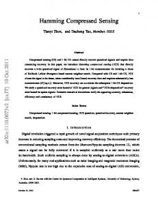
It is likely that the optimal sampling pattern depends on the spatial extent of the activated region. For example, denser sampling of central k-space lines might work better in studies with a larger activation area since the spatial Fourier transform of the activated area would have larger low frequency components. Preferential sampling of the central k-space lines might also be beneficial since most image intensities reside in the low k-space region. In 2D imaging, randomness was only present along the phase encoding (PE) direction. A full sampling pattern and two undersampling patterns are displayed in Fig. 1. Three undersampling patterns are as follows.
171 172
Gaussian + ky = 0 line (Gaussian) The undersampling pattern in Fig. 1B always samples the ky = 0 line and randomly samples the remaining lines according to a Gaussian probability distribution, A ⋅ exp(− n2y /2σ2), with standard deviation σ = 0.25Ny, where Ny is the number of PE steps and ny is the k-space line index ranging from −Ny/2 + 1 to Ny. The scaling factor A was adjusted so that the desired reduction factor was achieved. This pattern is denoted as Gaussian.
181
Please cite this article as: Zong, X., et al., Compressed sensing fMRI using gradient-recalled echo and EPI sequences, NeuroImage (2014), http:// dx.doi.org/10.1016/j.neuroimage.2014.01.045
162 163 164 165 166 167 168 169
173 174 175 176 177 178 179 180 Q2
182 183 184 185 186 187 188
3
R O
O
F
X. Zong et al. / NeuroImage xxx (2014) xxx–xxx
193 194
205
Stimulation paradigms
206
218
For simplicity, the number of images and the TR reported in this section refer to those in the fully sampled case. To compare CS and fully sampled data, both scans have the same scan time and stimulation pattern while the numbers of images are different. For example, for CS fMRI with R of 4, the number of images and the TR are 4 times and one fourth of the fully sampled case, respectively. For the periodic block-designed paradigm, each scan consists of 5 electrical stimulation trials, in which each trial consisted of 4 controls, 6 stimulations, and 20 control fullysampled images with a TR of 1.92 s. For the single-trial block-designed paradigm, each scan consists of a single trial of 15 controls, 8 stimulations, and 15 control fully-sampled images with a TR of 8 s. During the stimulation periods, an odor of amyl-acetate was delivered to the animals. The block-designed paradigms are illustrated in Fig. 1S.
219
Computer simulations
220 221
We first carried out computer simulations with the above stimulation paradigms to evaluate the dependence of the k–t FOCUSS performance on the k-space sampling pattern, spatial activation extent and temporal response shape. To evaluate the variability of the simulation results, the simulation was repeated 6 times with identical noise
207 208 209 210 211 212 213 214 215 216 217
222 223 224
C
E
R
R
201 202
N C O
199 200
U
197 198
T
203 204
Random (rand) A third undersampling pattern, not shown in Fig. 1, is to randomly sample ny with a constant probability over the whole ny range. This pattern is denoted as Rand. These undersampling patterns were re-generated for each image in repeated acquisitions. Computer simulations were first carried out to examine the performance of the three possible undersampling patterns in fMRI of S1 and OB, and in vivo experiments were performed with Gaussian and Rand + C6 patterns. When necessary, the reduction factor was reported by a number within parentheses following the pattern name.
195 196
distributions. In each simulation, a k-space dataset was generated in the following four steps. First, image series was generated by replicating a complex-valued, single-slice seed image. The seed images were taken from the S1 and OB fMRI studies (see later) with matrix size = 64 × 64, and were assumed to have a TR = 0.48 s and 2 s in S1 and OB studies, respectively, which are equal to the experimental TR values with R = 4. Second, the magnitudes of voxels within an activation region of interest (ROI) were modulated according to the hemodynamic response functions. The activation ROIs in S1 and OB (see contours in Figs. 2(A) and (B)) were defined based on the activation maps obtained in real experiments. The response functions were obtained by convoluting the stimulation patterns (on = 1 and off = 0) with canonical impulse response functions; gamma function in S1 and a single exponential function in OB. The resulting peak responses were assumed to be 1.5% and −8% in S1 and OB, respectively, as shown in Fig. 1S. Third, white noise was added to all voxels. The real and imaginary parts of the noise followed an identical Gaussian distribution for all voxels. Five noise levels were chosen with a different width for the noise distributions, resulting in the mean peak fMRI signal change to noise ratios (CNR) of 2.0, 1.5, 1.0, 0.5, and 0.3 in the activated S1 and OB ROIs. Fourth, the fully sampled data were simulated by retaining one of every four images in the series. For undersampled data, the image series were Fourier transformed to the k-space, randomly undersampled along PE with R = 4 according to the Gaussian, Rand + C6, and Rand patterns, and then reconstructed with k–t FOCUSS. The PE direction is assumed to be along the dorsal–ventral direction.
225 226
In vivo fMRI experiments
253
D
191 192
Random + 6 low k-space lines (rand + C6) The undersampling pattern in Fig. 1C always samples six central kspace lines corresponding to 5–10% of the 128 and 64 lines in full kspace, and randomly selects the remaining lines. This pattern is denoted as Rand + C6.
E
189 190
P
Fig. 1. Different sampling patterns for simulations and experiments. (A) Fully sampled (R = 1), (B) undersampled along the PE direction with a reduction factor (R) of 2. The sampling probability follows a Gaussian distribution with sampling of ky = 0 (Gaussian) (top panel) or is constant with the sampling of 6 central lines (Rand + C6) (bottom panel). (C) Same undersampling patterns as in (B) but with R of 4.
227 228 229 230 231 232 233 234 235 236 237 238 239 240 241 242 243 244 245 246 247 248 249 250 251 252
BOLD and CBV-weighted fMRI were carried out for S1 and OB activa- 254 tion studies, respectively, to evaluate the performance of in vivo CS– 255 fMRI applications. 256 Animal preparation and stimulation Eight male Sprague–Dawley rats weighing 240–450 g (Charles River Laboratories, Wilmington, MA, USA) were studied with approval by the University of Pittsburgh Animal Care and Use Committee; three for somatosensory cortex BOLD fMRI studies and five for olfactory bulb CBV-weighted fMRI. Animals were anesthetized with α-chloralose and
Please cite this article as: Zong, X., et al., Compressed sensing fMRI using gradient-recalled echo and EPI sequences, NeuroImage (2014), http:// dx.doi.org/10.1016/j.neuroimage.2014.01.045
257 258 259 260 261 262
X. Zong et al. / NeuroImage xxx (2014) xxx–xxx
R O
O
F
4
273 274 275 276 277 278 279 280 281 282 283 284 285 286
t1:1 t1:1
Table 1 Summary of fMRI experimental parameters.
U
N
287
1. The GRE sequence for S1 BOLD–fMRI had TE = 20 ms, and the time for acquiring one k-space line = 30 ms. Fully sampled data and CS data with R = 2 and R = 4 were acquired.
t1:1
Forepaw stimulation
t1:1
#1. GRE
#2. EPI
#3. GRE
64 × 64 × 1 20 × 20 × 2 mm3 1.92 s (R = 1) 0.96 s (R = 2) 0.48 s (R = 4) Full (3), Gaussian (3), Rand + C6 (3) Periodic block
128 × 128 × 2 30 × 30 × 4 mm3 2 s (R = 1; 2 shots); 1 s (R = 2; 1 shot)
64 × 64 × 9 7 × 7 × 4.5 mm3 8 s (R = 1) 2 s (R = 4)
Full (3), Gaussian (3), Rand + C6 (3) Periodic block
Full (5), Gaussian (2), Rand + C6 (5) Single-trial block
t1:1 t1:1
Matrix size FOV Image TR
t1:1
Sampling patterna t1:1 t1:1 t1:1
288
Data analysis
305
All CS data were reconstructed with k–t FOCUSS. Then, the t- and Fstatistics were calculated within the GLM framework using SPM8 (Wellcome Trust Centre for Neuroimaging, London, UK) software. A significance level of p ≤ 0.01 was used to define activated voxels.
306
CS data process with k–t FOCUSS To reconstruct the under-sampled simulated and experimental fMRI data, k–t FOCUSS with temporal FT and KLT was used. Parameter definitions can be found in Jung et al. (2009). Parameters for k–t FOCUSS with FT and KLT were: FOCUSS iteration number = 2, iteration number of conjugate gradient = 60, weighting matrix update power γ = 0.5, and regularization factor λ = 0.01. For k–t FOCUSS with KLT, the initial KLT matrix was calculated from images reconstructed by k–t FOCUSS with FT. After the reconstruction was finished, the KLT matrix was updated. The reconstruction and matrix updates were repeated three times. The iteration numbers were chosen empirically to ensure convergence and to achieve close-to-optimal activation maps. Before the CS reconstruction, the average of acquired k-space data across all of the image frames was subtracted from the raw data. After the reconstruction, the averaged images were added back to the reconstructed images at each time point (Jung et al., 2009).
310
E
D
2. High-resolution S1 BOLD–fMRI with the EPI sequence was performed with spectral width = 278 kHz. Two-shot fully sampled data (R = 1) and single-shot CS data with R = 2 were alternatively acquired. The echo time was 20 ms for full sampling, while for undersampling, due to the random skipping of some k-space lines, the echo time (time of ky = 0) had a mean of 20 ms, but varied with a standard deviation of 1–1.2 ms between images. For all EPI scans, a reference scan was acquired at the beginning of each scan with the same sequence but with the PE gradient turned off to partially correct for the phase inconsistency between the odd and even echoes. The correction was performed on a point-by-point basis after Fourier transform along the readout direction (Bruder et al., 1992). 3. High-resolution CBV-weighted OB GRE fMRI data were obtained after the intravenous injection of 15 mg Fe/kg Feraheme (AMAG Pharmaceuticals, Inc., MA) with TE = 8 ms and time for acquiring one k-space line for all slices = 125 ms. Fully sampled scans and CS scans with R = 4 were acquired.
T
C
271 272
Data acquisition All MRI experiments were performed on a 9.4 T/31 cm magnet equipped with an actively shielded 12-cm gradient set interfaced to a DirectDrive 2 console (Agilent Santa Clara, CA, USA). Single-loop surface coils with inner diameters of 2 cm and 1 cm were used in forepaw and odor stimulation studies, respectively. For the electrical stimulation study, the coil was placed above the skull near S1; while, for the odor stimulation study, the coil was dorsal to OB. The fMRI acquisition parameters are summarized in Table 1. Specifically, BOLD fMRI responses to forepaw stimulation were measured with GRE, and gradient-echo EPI sequences (#1–#2), while CBV fMRI responses to odor stimulation were measured with GRE (#3) only, since EPI in OB results in severe image distortion and signal dropout due to the presence of large B0 inhomogeneities. Specific acquisition and experimental parameters are described as follows:
E
270
R
268 269
R
266 267
urethane during the two studies, respectively. The detailed animal preparation procedure can be found in Poplawsky and Kim (in press) and Zong et al. (2012). For somatosensory cortex fMRI, the stimulation consists of electric current with amplitude = 1.4 mA, pulse duration = 333 μs, and repetition rate = 3 Hz delivered to the left forepaw. For olfactory bulb fMRI, odors of 5% amyl acetate in mineral oil and 100% mineral oil served as the stimulation and baseline control, respectively.
O
264 Q3 265
C
263
P
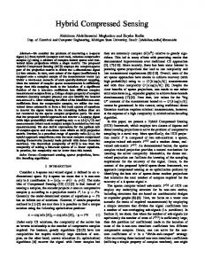
Fig. 2. Statistical t-value maps (p b 0.01) of S1 and OB calculated from the simulated block-designed fMRI data with different CNR levels. Different rows correspond to different sampling patterns. Green contour: ROI containing the true activation. Color bar: t-value.
Paradigm a
Odor stimulation
The numbers after pattern names are the number of animals scanned.
Please cite this article as: Zong, X., et al., Compressed sensing fMRI using gradient-recalled echo and EPI sequences, NeuroImage (2014), http:// dx.doi.org/10.1016/j.neuroimage.2014.01.045
289 290 291 292 293 294 295 296 297 298 299 300 301 302 303 304
307 308 309
311 312 313 314 315 316 317 318 319 320 321 322 323 324 325
X. Zong et al. / NeuroImage xxx (2014) xxx–xxx
347 348 349 350 351 352 353
354 355 356 357 358 359 360 361 362
ROC analysis of simulated data Receiver operator curves (ROC) of true positive fraction (TPF) versus false positive fraction (FPF) were calculated by varying the |t|-value threshold in defining activated regions. The TPF was calculated as the fraction of voxels above the threshold within the true activation ROI, while the FPF was calculated as the fraction of voxels above the threshold within a non-activation ROI. In order to consider the possible presence of increased false positive activations near the site of true activations due to spatial smoothing that may be introduced during
382
O
F
Results
R O
345 346
P
343 344
367 368 369 370 371 372 373 374 375 376 377 378 379 380 381
Computer simulations
383
Activation maps Fig. 2 displays the t-value maps calculated from the GLM analysis of the simulated fMRI data. All CS data were simulated with R = 4. At a CNR of 1 or above, clear and strong activations are detected in almost all voxels within the true activation ROI, regardless of the sampling pattern and sparsifying transform. At CNR of 0.3 and 0.5, the maps with Gaussian and Rand + C6 sampling patterns contain more activated voxels than those with Rand and full sampling. No obvious increase of false positive rates in the voxels surrounding the true activation ROI was observed, suggesting that no spatial smoothing was introduced during the reconstruction process. No noticeable difference is present between the maps reconstructed with KLT and FT (Fig. 2S). Therefore, only KLT maps are displayed in Fig. 2.
384
D
341 342
366
E
339 340
T
337 338
C
335 336
E
333 334
R
332
ROI-based analyses In the simulation, the ROI was defined as the assumed true activation area in both S1 and OB data. For S1 fMRI experiments, the ROI was defined as the cluster of voxels with p ≤ 0.01 and positive t-values in the expected S1 area contralateral to the stimulated forepaw in one fully sampled scan. For the OB experiments, the ROI was defined as voxels within OB with p ≤ 0.01 and positive t-values on the CS fMRI maps reconstructed with k–t FOCUSS with KLT, since the fully sampled maps have low sensitivity. ROI-averaged time courses were calculated for the block-designed simulated and experimental data to examine the effects of CS reconstruction on the temporal characteristics of the response. Also, the average peak intensity, noise level and mean t-value were computed from all voxels within each ROI. Voxel-wise noise levels were calculated as temporal standard deviations in the baseline images (0–8 s and 40–60 s for S1 and 0–120 s and 256–304 s for OB in each trial). The mean noise was calculated by averaging across scans and animals.
R
330 331
N C O
328 329
the reconstruction process, the non-activation ROI was defined as 363 one-voxel-thick band immediately surrounding the true activation 364 ROI. Then, areas under the ROC (AUR) were calculated. 365
GLM analysis The GLM analysis of simulated data was carried out with the same reference response functions used for generating the simulated data. For the periodic block-designed scans in S1, the GLM analysis was performed for each scan. For the single-trial block-designed OB scans, the GLM analysis was performed on three concatenated scans. The covariance structure in the noise was estimated by the “spm_ar_reml.m” function in SPM8 which provides an estimate of the AR coefficient for the residual temporal correlation. The six simulated data sets were analyzed individually and the results averaged. For the GLM analysis of the experimental data, we used reference response functions by convoluting canonical IRFs with the stimulation patterns. For S1, the IRF was generated with the “spm_hrf.m” in SPM with an onset delay of 1.3 s (Hillman et al., 2007). For OB, the IRF was given by f(t) = exp(−t/τ), with τ = 22 s. In S1 fMRI, each scan was analyzed separately. In OB fMRI studies, three consecutive scans with the same sampling pattern were concatenated in each animal, and multiple GLM analyses (each with three concatenated scans) were performed for each pattern. The design matrix consisted of a column of reference responses and two columns modeling constant and linearly drifting baselines. Separate baseline columns were used for different scans to account for possible baseline image intensity changes across scans. The covariance structures of the noise in all analyses were estimated by the function “spm_reml.m” in SPM8. In addition, for two animals with 9 fully sampled scans, all scans were concatenated for GLM analysis in order to obtain activation maps with higher sensitivity. Such full sampling maps can serve as a better reference for evaluating the activation areas observed in the CS–fMRI maps.
U
326 327
5
Fig. 3. Mean fMRI responses in the truly activated ROI in the simulated fMRI data with CNR = 2.0 and 0.3. (A) S1 (first and second columns) and (B) OB data (third and fourth columns) were averaged over 30 and 18 trials, respectively, for four k-space sampling patterns. Patterns in rows 1–4: full, Gaussian, Rand + C6, and Rand. The CS data were reconstructed by k–t FOCUSS with KLT.
Please cite this article as: Zong, X., et al., Compressed sensing fMRI using gradient-recalled echo and EPI sequences, NeuroImage (2014), http:// dx.doi.org/10.1016/j.neuroimage.2014.01.045
385 386 387 388 389 390 391 392 393 394 395 396
X. Zong et al. / NeuroImage xxx (2014) xxx–xxx
P
R O
O
F
6
C
O
R
R
E
C
T
E
shapes from the undersampled data with R = 4 closely match those of the fully sampled ones, their peak heights were reduced, depending on the sampling pattern and CNR. The reduction is the largest for random sampling and the least for Rand + C6, consistent with higher
N
399 400
Time courses and noise characteristics Fig. 3 shows time courses from the true activation ROI in the simulated data. Time courses appear very similar between CS data reconstructed with FT (data not shown) and KLT. While the response
U
397 398
D
Fig. 4. Baseline noise levels (A–B) and areas under the receiver operator curves for activation detection (C–D) in simulated block-designed data with different CNRs and four sampling patterns (different colors). (A) and (C) for S1 and (B) and (D) for OB. The CS data were reconstructed by k–t FOCUSS with KLT.
Fig. 5. Experimental statistical t-value maps of two rats responding to forepaw stimulation using block-designed GRE fMRI with different sampling patterns and acceleration factors. Color functional maps were overlaid on baseline GRE images. Images were reconstructed by using k–t FOCUSS with FT and KLT. Note that the number of spuriously activated voxels is reduced with KLT.
Please cite this article as: Zong, X., et al., Compressed sensing fMRI using gradient-recalled echo and EPI sequences, NeuroImage (2014), http:// dx.doi.org/10.1016/j.neuroimage.2014.01.045
401 402 403 404
7
R O
O
F
X. Zong et al. / NeuroImage xxx (2014) xxx–xxx
413 414 415 416 417
E
T
411 412
C
409 410
Since the Rand + C6 and Gaussian patterns provide better sensitivity 426 in both S1 and OB data than the Rand pattern, only these two 427 undersampling patterns were used in the actual experiments. 428
E
407 408
sampling density of low k-space lines in the latter. On the other hand, the noise level is reduced in the CS data as shown in Fig. 4(A) and (B). Note that the noise levels are different between the OB and S1 at the same CNR because of the different peak response amplitudes. The ReML analysis of the temporal noise suggests that k–t FOCUSS did not introduce false temporal correlations into the reconstructed images. The AR coefficients estimated for all GLM analyses were very small (~ 0.02) for all sampling patterns, noise levels, and sparsifying transforms, and did not differ between the fully sampled and undersampled cases. For the fully sampled images, no temporal correlation is expected since white noise was added to the data.
R
405 406
D
P
Fig. 6. Experimental statistical t-value maps of two rats responding to amyl acetate odor stimulation using experimental block-designed GRE fMRI with full sampling and undersampling of R of 4. Color functional maps were overlaid on T2-weighted images. The white arrows indicate areas with false activation and opposite signal change. Undersampled images were reconstructed with k–t FOCUSS with KLT.
In vivo block-designed experiments with the GRE sequence
429
Robust activation in S1 by forepaw stimulation is detected in both fully sampled and CS scans as shown in Fig. 5 in two representative rats. In general, there is an increase in the t-values when the reduction factor is increased, while the number of activated voxels remains similar. Compared to the fully sampled fMRI maps, some CS functional maps show increased numbers of false activations outside of S1, which appear to be reduced for the KLT reconstruction. Fig. 6 displays representative thresholded t-value maps responding to strong odor stimulation. The CS fMRI maps show a remarkable increase in the number of activated voxels compared to the fully sampled fMRI maps, even when comparing to the fully sampled maps with three times the number of concatenated trials. Nevertheless, the activation centers with high t-values co-localize well between the 3-trial CS–fMRI maps and the 9-trial fully sampled maps. Due to the increased sensitivity with undersampling, broad activation surrounding the activation centers in the middle layers of the OB is observed, consistent
430
t2:2 t2:2
Table 2 Percent signal change, noise level, the number of activated voxels, and t-value in block-designed S1 and OB fMRI obtained with the GRE sequencea.
422 423
t2:2
N C O
420 421
Area
U
418 419
R
424 425
ROC analysis To assess the sensitivity of CS fMRI, AUR for the simulated S1 and OB data are displayed in Fig. 4(C) and (D). A higher AUR indicates higher sensitivity at the same false positive rates. At the highest CNR, performances of the different sampling patterns appear similar. However, as the CNR decreases, the Gaussian and Rand + C6 patterns provide higher sensitivities than the Rand and full sampling patterns. The AURs for the Rand + C6 pattern are either similar to or greater than those for the Gaussian pattern in most cases, suggesting that sampling of several low ky lines is more beneficial than sampling a single line at ky = 0.
Sampling pattern
Percent change
Noise level
t2:2 t2:2 t2:2 t2:2 t2:2 t2:2 t2:2 t2:2 t2:2 t2:2
S1
Full R=2 R=4
OB
Full R=4
Gaussian Rand + C6 Gaussian Rand + C6 Gaussian Rand + C6
6.5 4.1 3.3 2.2 2.1 −4.2 −3.6 −4.1
± ± ± ± ± ± ± ±
2.2% 1.3% 1.2% 0.5% 0.6% 0.5% 0.3% 0.4%
5.4 5.1 5.0 3.8 4.1 14.5 10.3 9.8
± ± ± ± ± ± ± ±
0.4% 0.5% 0.3% 0.4% 0.4% 2.8% 1.4% 2.4%
# of active voxels
t-Value
Positive only
Positive + negative
51 53 59 50 77 1433 3985 5113
69 80 90 95 117 1519 4442 5451
± ± ± ± ± ± ± ±
13 11 8 11 18 351 489 717
± ± ± ± ± ± ± ±
17 43 32 28 33 370 71 751
4.8 5.1 5.1 5.4 5.6 3.1 3.9 4.9
± ± ± ± ± ± ± ±
1.0 0.8 0.5 0.6 0.6 0.2 0.3 0.8
a Percent change, noise level, and t-value were obtained from the ROI, while # of activated voxels were calculated from entire images. “Positive only” and “Positive + negative” refer to the sign of t values of the activated voxels (p b 0.01). Results in S1 were first obtained from each scan and then averaged across 6 scans (n = 6). Results in OB with Rand + C6 and full patterns were first obtained from GLM analysis of 3 concatenated scans and then averaged across different concatenated sets (n = 8). Results in OB with Gaussian sampling were first obtained from GLM analysis of 3 concatenated scans and then averaged across different concatenated sets (n = 4). The errors are standard deviations.
Please cite this article as: Zong, X., et al., Compressed sensing fMRI using gradient-recalled echo and EPI sequences, NeuroImage (2014), http:// dx.doi.org/10.1016/j.neuroimage.2014.01.045
431 432 433 434 435 436 437 438 439 440 441 442 443 444 445
8
X. Zong et al. / NeuroImage xxx (2014) xxx–xxx Table 3 Percent signal change, noise level, and the number of activated voxels in high-resolution S1 fMRI obtained with the EPI sequencea.
Full R=2
Percent change
Noise level
# of activated pixels
t3:3
3.9 ± 1.3% 3.2 ± 0.7%
1.1 ± 0.5% 5.5 ± 1.0%
96 ± 34 75 ± 24
t3:3 t3:3
a Results were first obtained from each scan and then averaged across 9 scans (n = 9). The errors are standard deviations.
461 462 463 464 465 466 467 468 469 470 471 472 473 474 475
477
Discussion
489
D
P
R O
O
F
Fig. 8 shows activation maps obtained from fully sampled, two-shot data and undersampled, one-shot data. Despite the sensitivity of EPI to field inhomogeneities and off-resonance artifacts, the images reconstructed from undersampled EPI data have similar artifact levels as the fully sampled two-shot data (see background gray images). However, the activation maps calculated from the CS data have a reduced number of activated voxels, in contrast to those with the GRE sequence. The group-averaged mean response amplitude of the activated voxels, noise levels, and number of active voxels are listed in Table 3 for full and Rand + C6 (R = 2) sampling patterns. There is a large increase in noise levels when undersampling is applied in the EPI sequence, which might explain the sensitivity reduction in the undersampled data.
478 479 480 481 482 483 484 485 486 487 488
Dependence on the sampling pattern
490
Our simulation results showed that patterns of Gaussian and random sampling with full sampling of some center k-space lines outperform the fully random sampling pattern. Note that most of the high magnitude data points reside around the low k-space region, so the SNR penalty is more significant when skipping k-space data here. However, a greater acquisition of k-space center lines will bias the reconstruction toward the down-sampled low frequency component and will result in a blurring of the activation foci. Therefore, a balance between the center and edge k-space line acquisitions is necessary to optimize the performance of CS–fMRI data reconstruction, which appears to be the case for both the Gaussian and Rand + C6 patterns employed in our experiments. Also, the k–t FOCUSS algorithm is a re-weighted norm algorithm, so the convergence speed depends on the initial estimate. The Gaussian and Rand + C6 patterns can provide a reasonable, low resolution reconstruction that accelerates the convergence of k–t FOCUSS.
491
CS reconstruction algorithm and temporal correlation
507
T
C
459 460
E
457 458
R
455 456
R
453 454
O
452
C
450 451
N
448 449
with earlier glucose uptake measurements (Johnson et al., 1998; Sharp et al., 1977) and our previous fMRI studies with extensive signal averaging (Poplawsky and Kim, in press). In some rats, false activation with opposite signal change was observed in the CS–fMRI maps, as indicated by the white arrows in Fig. 6. To study the temporal characteristics of the functional responses measured by CS–fMRI, the group-averaged response time courses were obtained from the S1 and OB activation ROIs. Consistent with the simulation results, the CS data had reduced response amplitudes and a greater reduction was observed at R = 4 compared to R = 2 (data not shown). The response amplitude, voxel-wise noise level, number of active voxels, and mean t-value are compared for S1 and OB studies. The group-averaged values are given in Table 2. The CNR in S1 and OB block-designed experiments was found to be 1.2 and 0.3, respectively, in the fully sampled data. When R increases, both the response amplitude and noise level decrease as seen in the simulation data (Figs. 3 and 4A–B). While the numbers of activated voxels are similar across reduction factors in S1, CS greatly increases the number of activated voxels in OB compared to the fully sampled data. These differential sensitivities in CS–fMRI can be partly explained by the CNR difference in S1 and OB data, which is consistent with simulation data (Figs. 4C–D). Furthermore, the average t-values within the ROI increases at higher reduction factor in both S1 and OB, also consistent with simulation. To confirm that k–t FOCUSS did not introduce temporal noise correlations, the autocorrelation functions were estimated using the SPM ^ in Eq. (2)) for the block-designed S1 fMRI data (Fig. 7). procedure (V Note that the TR is 1.92 s, 0.96 s, and 0.48 s for R = 1, 2, and 4, respectively. The autocorrelation function for R = 4 is concentrated mostly around zero, suggesting that highly accelerated fMRI acquisition reduces temporal correlations.
476
492 493 494 495 496 497 498 499 500 501 502 503 504 505 506
Although no periodicity is present in the hemodynamic responses of 508 the single trial, k–t FOCUSS with FT can still recover activation maps 509 with improved sensitivity from undersampled k-space data. A plausible 510
U
446 447
t3:3
In vivo block-designed experiments with 2D-EPI
E
Fig. 7. Temporal autocorrelation functions of the reconstructed time series with various sampling patterns and sampling rates for averaged, block-designed, GRE S1 fMRI data. Only results for k–t FOCUSS with KLT are shown here, since k–t FOCUSS with FT produced similar results.
t3:3 t3:3 t3:3
Fig. 8. EPI-based fMRI maps of two rats responding to forepaw stimulation obtained from block-designed data with full and Rand + C6 (R = 2) sampling patterns. Color maps were overlaid on the corresponding baseline EPI images.
Please cite this article as: Zong, X., et al., Compressed sensing fMRI using gradient-recalled echo and EPI sequences, NeuroImage (2014), http:// dx.doi.org/10.1016/j.neuroimage.2014.01.045
X. Zong et al. / NeuroImage xxx (2014) xxx–xxx
explanation is that, due to the relatively slow hemodynamic response compared to the image acquisition rate (1/TR), FT of the time course has large coefficients concentrating mostly in the low frequency range and, thus, FT can still serve as an effective sparsifying transform. One could be concerned that better temporal resolution could potentially increase temporal correlation. Our interest for statistical analy^ sis is on the long range correlation which makes the structure of the V
press)). Third, the CS–fMRI activation patterns are consistent with ear- 575 lier glucose uptake measurements using the same odor (Johnson et al., 576 1998; Sharp et al., 1977). 577
580 581
550
matrix less diagonal. The reason that the long range correlation is more important than the frame-wise correlation is that it reduces the EDF (Friston et al., 2011). As discussed in the Statistical analysis section, it is well known that the reduced EDF increases the threshold of the t-statistic for the same p-value, which makes the t-test less sensitive (Friston et al., 2011). We believe that the long range correlation does not increase in CS due to the following reasons. First, as the acceleration factor increases, the temporal resolution is improved. Some common sources of noise that can introduce serial correlations, like hardware-related lowfrequency drifts, oscillatory fluctuations from respiration and cardiac pulsation, and residual movement artifacts not accounted for by image registration (Boynton et al., 1996; Friston et al., 1994; Weisskoff et al., 1993; Woolrich et al., 2001), can be reduced by improving the temporal resolution. Second, the CS reconstruction algorithm itself exploits the temporal redundancy to improve the reconstruction results. More specifically, the k–t FOCUSS with KLT exploits the sparsity in the Karhunen– Loeve transform (KLT) domain, which is known as the best de-correlator (Jain, 1989). Hence, the reweighted norm procedure suppresses the potential correlation in the background areas, which may result in the reduction of serial correlation. Consequently, the reduction of the serial correlation increases the EDF, which makes the statistical test more efficient. Reduction of the temporal correlation is another reason to justify the usefulness of CS–fMRI. Increased false negative changes (FPF) are sometimes observed in the experimental CS–fMRI maps (Figs. 5 and 6), which might compromise the sensitivity gain offered by CS–fMRI. Interestingly, the false activation appears less severe in KLT maps in Fig. 5. In addition, such increased false activations are absent in simulated CS–fMRI maps in Fig. 2. The origin of the increased FPF in experimental maps may be related to the presence of baseline drifts in the experimental data that were also non-periodic and, thus, can be better estimated with KLT. However, this phenomenon requires further investigation.
551
Discrepancy of sensitivity increase in S1 and OB
552 553
Undersampling leads to a large increase in the number of activated voxels in OB for a single-trial block paradigm, while, in S1, no obvious sensitivity increase is observed with undersampling. This difference may be explained by the CNR differences between the S1 and OB fMRI studies. According to Fig. 4C–D, the sensitivity gain by CS is only noticeable when CNR is ≤ 0.5. Experimental CNR is 1.2 in S1 and 0.3 for OB, which can explain the differential functional sensitivity gains. We note that the CNR threshold for better performance with CS depends on the number of trials and stimulation duration. Although no sensitivity gain is observed with CS in our study for CNR ≥1 due to the already very high sensitivity of the fully sampled data, t-values increase with CS–fMRI compared to full sampling at all CNRs (Figs. 2 and 5). In addition, the sensitivity gain could increase when a smaller number of trials or shorter stimulation durations are used, even at CNR ≥ 1. Under such experimental conditions, CS–fMRI can still provide sensitivity enhancement. Furthermore, the increased sensitivity in OB CS–fMRI is unlikely an artifact of k–t FOCUSS reconstruction. First, our simulation results demonstrated that no increased false positive rates are introduced by undersampling for k–t FOCUSS reconstruction. Second, although the true activated area is not known a priori for in vivo study, the CS–fMRI activation maps are similar to those obtained from fully sampled data with a large number of trials (see Fig. 6 and Poplawsky and Kim (in
532 533 534 535 536 537 538 539 540 541 542 543 544 545 546 547 548 549
554 555 556 557 558 559 560 561 562 563 564 565 566 567 568 569 570 571 572 573 574 Q5
Relevance to human sparsely sampled fMRI studies
625
EPI is a common imaging sequence for human fMRI studies. Due to the availability of conventional acceleration techniques, such as parallel imaging and multi-band excitation, on human scanners, the combination of EPI with these techniques allows sufficient temporal resolution for measuring hemodynamic responses. The large increase of noise in CS EPI data would reduce or eliminate the potential sensitivity gain offered by further increased temporal resolution with CS. However, as demonstrated in Jung and Ye (2009), if the additional noises are controlled during accelerated acquisition, CS–fMRI may be a useful tool for EPI–fMRI. Therefore, novel techniques to reduce the temporal noise from irregular sampling need to be investigated further to validate
626 627
O
F
579
R O
530 531
We found a large increase in sensitivity when applying CS to the GRE sequence, consistent with our simulation results. However, there appears to be no sensitivity gain when CS is applied to the EPI sequence. This difference can be explained by the difference in CNRs and by the additional noises introduced by the random sampling in the EPI sequence, which is absent in the GRE sequence. First, CNR is N2.0 for fully-sampled, two-shot EPI data (Table 3), but 0.3 to 1.2 for GRE data (Table 2). The sensitivity gain by CS is minimal when CNR ≥ 1 (see Fig. 4C–D). Hence, the advantages of CS–fMRI may not be as pronounced for EPI sequences with large CNR. Second, the temporal noise for images reconstructed from the undersampled EPI data is larger than for the fully sampled data (Table 3). However, the noise levels for images reconstructed from the undersampled GRE and simulated data were much lower than those reconstructed from the fully sampled data (Table 2 and Figs. 4A–B). Thus, such additional increases in noise that are unique to EPI reduce the potential sensitivity gain offered by CS. There are several possible sources of the temporal noise increases in undersampled EPI data. First, imperfections of PE blips can introduce errors in the ky values. Since the sampling pattern varies from image to image, such errors are image-dependent and introduce additional temporal fluctuations in the reconstructed images. In comparison, these imperfections and resulting errors in ky values remain constant in the regular, fully-sampled EPI and in both undersampled and regular GRE sequences. A second source of error in the undersampled EPI sequence is the mismatch between the odd and even echoes, which may not be completely corrected by the reference scans acquired at the beginning of each scan. In regular EPI, such mismatches produce the well-known N/2 ghosting artifact and remains constant across images. However, in the undersampled EPI, a k-space line at a certain ky value is randomly encoded by either an odd or even echo, depending on the sampling pattern at that time point. Therefore, additional temporal fluctuations are introduced. Third, off-resonance, due to local field inhomogeneities, produces a constant image shift along the phase-encoding direction with the regular EPI sequence as a result of off-resonance-induced phase accumulation that linearly depends on ky. However, when random undersampling is applied, the phase accumulation becomes an irregular function of ky, which may result in blurring and a shift of the image intensities. Thus, the image to image variation of this effect introduces additional temporal noise to the affected image regions. Fourth, because of a random change in TE among the images, the image intensity would vary due to the T2⁎ decay. Assuming a T2⁎ value of 27 ms, as is typically found in the in vivo rat brain at 9.4 T (Kim and Kim, 2011), the TE variation of 1 ms in our sequence would introduce nearly a 4% signal fluctuation. This fluctuation can be reduced if sampling patterns with a constant TE are used, such as measuring the same number of ky values before measuring ky = 0 for all images.
P
528 529
578
D
526 527
GRE vs. EPI
E
524 525
T
522 523
C
520 Q4 521
E
518 519
R
517
R
515 516
N C O
513 514
U
511 512
9
Please cite this article as: Zong, X., et al., Compressed sensing fMRI using gradient-recalled echo and EPI sequences, NeuroImage (2014), http:// dx.doi.org/10.1016/j.neuroimage.2014.01.045
582 583 584 585 586 587 588 589 590 591 592 593 594 595 596 597 598 599 600 601 602 603 604 605 606 607 608 609 610 611 612 613 614 615 616 617 618 619 620 621 622 623 624
628 629 630 631 632 633 634 635 636
679
Acknowledgments
680
685
This work was partially supported by the National Institutes of Health (NS07391, MH18273, EB003324, and EB003375), the Institute for Basic Science (IBS) (EM1305), and the Korea Science and Engineering Foundation Grant funded by the Korean Government (MEST) (No. 2009-0081089). In addition, we thank Dr. Ping Wang for experimental support, and Kristy Hendrich for the 9.4 T scanner maintenance.
686
References
687 688 689 690 691 692 693 694 695 696 697
Boynton, G.M., Engel, S.A., Glover, G.H., Heeger, D.J., 1996. Linear systems analysis of functional magnetic resonance imaging in human V1. J. Neurosci. 16, 4207–4221. Bruder, H., Fischer, H., Reinfelder, H.E., Schmitt, F., 1992. Image reconstruction for echo planar imaging with nonequidistant k-space sampling. Magn. Reson. Med. 23, 311–323. Candes, E., Romberg, J., Tao, T., 2006. Robust uncertainty principles: exact signal reconstruction from highly incomplete frequency information. IEEE Trans. Inf. Theory 52, 489–509. Donoho, D.L., 2006. Compressed sensing. IEEE Trans. Inf. Theory 52, 1289–1306. Feng, L., Otazo, R., Jung, H., Jensen, J.H., Ye, J.C., Sodickson, D.K., Kim, D., 2011. Accelerated cardiac T2 mapping using breath-hold multiecho fast spin-echo pulse sequence with k–t FOCUSS. Magn. Reson. Med. 65, 1661–1669.
666 667 668 669 670 671 672 673 674 675 676
681 682 683 684
C
664 665
E
658 659
R
656 657
R
654 655
O
652 653
C
650 651
N
648 649
U
646 647
F
677 678
This paper investigated the performances of CS–fMRI using blockdesign stimulation experiments for rat models using 9.4-T MRI. Specifically, accelerated acquisition and CS-reconstruction using k–t FOCUSS were studied extensively using GRE and EPI pulse sequences with real k-space undersampling and rigorous statistical analysis. Despite the potential concerns about CS–fMRI, our results showed that the improved temporal resolution from CS–fMRI reduces the serial correlation in the fMRI image and improves the statistical performance of activation detection. We also found that center-weighted random sampling patterns were preferred over the purely random sampling patterns. Similarly, CS–fMRI should also be useful for rapid event-related fMRI experiments. In summary, our results confirm that CS–fMRI is a viable tool that has a great potential to improve the performance of fMRI studies, although the potential presence of increased FPF should be carefully evaluated. Supplementary data to this article can be found online at http://dx. doi.org/10.1016/j.neuroimage.2014.01.045.
644 645
O
663
643
R O
Conclusions
641 642
P
662
639 640
Frahm, J., Merboldt, K.D., Hanicke, W., 1993. Functional MRI of human brain activation at high spatial resolution. Magn. Reson. Med. 29, 139–144. Friston, K.J., P. J., Turner, R., 1994. Analysis of functional MRI time-series. Hum. Brain Mapp. 1, 153–171. Friston, K.J., Ashburner, J.T., Kiebel, S.J., Nichols, I.E., Penny, W.D., 2011. Statistical Parametric Mapping: The Analysis of Functional Brain Images. Academic Press. Graser, H., Smith, S., Tier, B., 1987. A derivative-free approach for estimating variance components in animal models by restricted maximum likelihood. J. Anim. Sci. 1987, 1362–1370. Harville, D., 1977. Maximum likelihood approaches to variance component estimation and to related problems. J. Am. Stat. Assoc. 72, 320–338. Hillman, E.M., Devor, A., Bouchard, M.B., Dunn, A.K., Krauss, G.W., Skoch, J., Bacskai, B.J., Dale, A.M., Boas, D.A., 2007. Depth-resolved optical imaging and microscopy of vascular compartment dynamics during somatosensory stimulation. Neuroimage 35, 89–104. Holland, D.J., Liu, C., Song, X., Mazerolle, E.L., Stevens, M.T., Sederman, A.J., Gladden, L.F., D'Arcy, R.C., Bowen, C.V., Beyea, S.D., 2013. Compressed sensing reconstruction improves sensitivity of variable density spiral fMRI. Magn. Reson. Med. Hu, Y., Lingala, S.G., Jacob, M., 2012. A fast majorize–minimize algorithm for the recovery of sparse and low-rank matrices. IEEE Trans. Image Process. 21, 742–753. Jain, A.K., 1989. Fundamentals of Digital Image Processing. Prentice-Hall, Englewood Cliffs. Jeromin, O., Pattichis, M.S., Calhoun, V.D., 2012. Optimal compressed sensing reconstructions of fMRI using 2D deterministic and stochastic sampling geometries. Biomed. Eng. Online 11, 25. Johnson, B.A., Woo, C.C., Leon, M., 1998. Spatial coding of odorant features in the glomerular layer of the rat olfactory bulb. J. Comp. Neurol. 393, 457–471. Jung, H., Ye, J.C., 2009. Performance evaluation of accelerated functional MRI acquisition using compressed sensing. IEEE Int. Symp. Biomed. Imag. 702–705. Jung, H., Ye, J., 2010. Motion estimated and compensated compressed sensing dynamic magnetic resonance imaging: what we can learn from video compression techniques. Int. J. Imaging Syst. Technol. 20, 81–98. Jung, H., Ye, J.C., Kim, E.Y., 2007. Improved k–t BLAST and k–t SENSE using FOCUSS. Phys. Med. Biol. 52, 3201–3226. Jung, H., Sung, K., Nayak, K.S., Kim, E.Y., Ye, J.C., 2009. k–t FOCUSS: a general compressed sensing framework for high resolution dynamic MRI. Magn. Reson. Med. 61, 103–116. Jung, H., Park, J., Yoo, J., Ye, J.C., 2010. Radial k–t FOCUSS for high-resolution cardiac cine MRI. Magn. Reson. Med. 63, 68–78. Kenward, M.G., Roger, J.H., 1997. Small sample inference for fixed effects from restricted maximum likelihood. Biometrics 53, 983–997. Kida, I., Xu, F., Shulman, R.G., Hyder, F., 2002. Mapping at glomerular resolution: fMRI of rat olfactory bulb. Magn. Reson. Med. 48, 570–576. Kim, T., Kim, S.-G., 2011. Cerebral arterial blood R2* and volume measurements during stimulation. Proc. Intl. Soc. Mag. Reson. Med. 19, 1546. Lam, F., Zhao, B., Liu, Y., Liang, Z.-P., Weinei, M., Schuff, N., 2013. Accelerated fMRI using low-rank model and sparsity constraints. Proc. Intl. Soc. Mag. Reson. Med. 21, 2620. Lingala, S.G., Hu, Y., DiBella, E., Jacob, M., 2011. Accelerated dynamic MRI exploiting sparsity and low-rank structure: k–t SLR. IEEE Trans. Med. Imaging 30, 1042–1054. Lu, W., Vaswani, N., 2011. Modified-cs-residual for recursive reconstruction of highly undersampled functional mri sequences. Proc. IEEE Int. Conf. Imag Proc. (ICIP). Lustig, M., Santos, J., Donoho, D., Pauly, J., 2006. kt SPARSE: high frame rate dynamic MRI exploiting spatio-temporal sparsity. Proc. Intl. Soc. Mag. Reson. Med. 14, 2420. Nguyen, H.M., Glover, G.H., 2013. A modified generalized series approach: application to sparsely sampled FMRI. IEEE Trans. Biomed. Eng. 60, 2867–2877. Ogawa, S., Tank, D.W., Menon, R., Ellermann, J.M., Kim, S.G., Merkle, H., Ugurbil, K., 1992. Intrinsic signal changes accompanying sensory stimulation: functional brain mapping with magnetic resonance imaging. Proc. Natl. Acad. Sci. U. S. A. 89, 5951–5955. Ojemann, J.G., Akbudak, E., Snyder, A.Z., McKinstry, R.C., Raichle, M.E., Conturo, T.E., 1997. Anatomic localization and quantitative analysis of gradient refocused echo-planar fMRI susceptibility artifacts. Neuroimage 6, 156–167. Olman, C.A., Davachi, L., Inati, S., 2009. Distortion and signal loss in medial temporal lobe. PLoS One 4, e8160. Poplawsky, A., Kim, S.-G., 2014. Layer-dependent BOLD and CBV-weighted fMRI responses in the rat olfactory bulb. Neuroimage (2013, in press). Searle, S., 1979. Notes on Variance Component Estimation: A Detailed Account of Maximum Likelihood and Kindred Methodology. Biometrics Unit, Cornell University. Sharp, F.R., Kauer, J.S., Shepherd, G.M., 1977. Laminar analysis of 2-deoxyglucose uptake in olfactory bulb and olfactory cortex of rabbit and rat. J. Neurophysiol. 40, 800–813. Usman, M., Prieto, C., Schaeffter, T., Batchelor, P.G., 2011. k–t Group sparse: a method for accelerating dynamic MRI. Magn. Reson. Med. 66, 1163–1176. Weisskoff, R., Baker, J., Belliveau, J., Davis, T., Kwong, K., Cohen, M., Rosen, B., 1993. Power spectrum analysis of functionally-weighted MR data: what's in the noise. Proc. Soc. Magn. Reson. Med. 1, 7. Woolrich, M.W., Ripley, B.D., Brady, M., Smith, S.M., 2001. Temporal autocorrelation in univariate linear modeling of FMRI data. Neuroimage 14, 1370–1386. Xu, F., Kida, I., Hyder, F., Shulman, R.G., 2000. Assessment and discrimination of odor stimuli in rat olfactory bulb by dynamic functional MRI. Proc. Natl. Acad. Sci. U. S. A. 97, 10601–10606. Zhang, T., Chowdhury, S., Lustig, M., Barth, R.A., Alley, M.T., Grafendorfer, T., Calderon, P.D., Robb, F.J., Pauly, J.M., Vasanawala, S.S., 2013. Clinical performance of contrast enhanced abdominal pediatric MRI with fast combined parallel imaging compressed sensing reconstruction. J. Magn. Reson. Imaging. Zhao, B., Haldar, J.P., Brinegar, C., Liang, Z.P., 2010. Low rank matrix recovery for real-time cardiac MRI. IEEE Int. Symp. Biomed. Imag. 996–999. Zong, X., Kim, T., Kim, S.G., 2012. Contributions of dynamic venous blood volume versus oxygenation level changes to BOLD fMRI. Neuroimage 60, 2238–2246.
T
660 661
the efficacy of CS–fMRI for human study. On the other hand, the GRE sequence may still be useful for fMRI of human brain regions with large B0 field inhomogeneities, such as the medial temporal lobe, orbital frontal cortex, and olfactory bulb (Ojemann et al., 1997; Olman et al., 2009), where CS can be applied in combination with the other acceleration techniques for increased temporal resolution and sensitivity, as demonstrated in a recent dynamic contrast enhanced MRI study (Zhang et al., 2013). Therefore, GRE based CS–fMRI can be directly used for human brain study as an extension of this work. Several studies have demonstrated the feasibility of sparsely sampled fMRI with reduction factors up to R = 5 (Holland et al., 2013; Jeromin et al., 2012; Jung and Ye, 2009; Lam et al., 2013; Lu and Vaswani, 2011; Nguyen and Glover, 2013). Except in Nguyen and Glover (2013), most of the studies exploited retrospectively undersampled data and/or had a fixed TR at all reduction factors. Therefore, undersampling did not translate to an increased number of images or an increased sensitivity for the same experimental durations in these studies. In Nguyen and Glover (2013), a variable density spiral sequence was implemented with R = 4, which resulted in an increased statistical power compared to the fully sampled data, consistent with our results. k–t FOCUSS was also examined and was found to introduce high-frequency ringing artifacts, which are not observed in our study. This discrepancy may be explained by the absence of random variations of the k-space sampling pattern across images in Nguyen and Glover (2013), which is an important prerequisite for the application of k–t FOCUSS.
D
637 638
X. Zong et al. / NeuroImage xxx (2014) xxx–xxx
E
10
Please cite this article as: Zong, X., et al., Compressed sensing fMRI using gradient-recalled echo and EPI sequences, NeuroImage (2014), http:// dx.doi.org/10.1016/j.neuroimage.2014.01.045
698 699 700 Q6 701 702 703 704 705 706 707 708 709 710 711 712 713 714 715 Q7 716 717 718 719 720 721 722 723 724 725 726 727 728 729 730 731 732 733 734 735 736 737 738 739 740 741 742 743 744 745 746 747 748 749 750 751 752 753 754 755 756 757 758 759 Q8 760 761 762 763 764 765 766 767 768 769 770 771 772 773 774 775 776 777 778 Q9 779 780 781 782