Compressed Sensing Makes Every Pixel Count

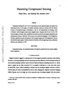
One is Enough. A photograph taken by the “single-pixel camera” built by Richard Baraniuk and Kevin Kelly of Rice University. (a) A photograph of a soccer ball, taken by a conventional digital camera at 64 × 64 resolution. (b) The same soccer ball, photographed by a single-pixel camera. The image is derived mathematically from 1600 separate, randomly selected measurements, using a method called compressed sensing. (Photos courtesy of R. G. Baraniuk, Compressive Sensing [Lecture Notes], Signal c Processing Magazine, July 2007. 2007 IEEE.)

114

What’s Happening in the Mathematical Sciences

Compressed Sensing Makes Every Pixel Count

T

rash and computer files have one thing in common: compact is beautiful. But if you’ve ever shopped for a digital camera, you might have noticed that camera manufacturers haven’t gotten the message. A few years ago, electronic stores were full of 1- or 2-megapixel cameras. Then along came cameras with 3-megapixel chips, 10 megapixels, and even 60 megapixels. Unfortunately, these multi-megapixel cameras create enormous computer files. So the first thing most people do, if they plan to send a photo by e-mail or post it on the Web, is to compact it to a more manageable size. Usually it is impossible to discern the difference between the compressed photo and the original with the naked eye (see Figure 1, next page). Thus, a strange dynamic has evolved, in which camera engineers cram more and more data onto a chip, while software engineers design cleverer and cleverer ways to get rid of it. In 2004, mathematicians discovered a way to bring this “arms race” to a halt. Why make 10 million measurements, they asked, when you might need only 10 thousand to adequately describe your image? Wouldn’t it be better if you could just acquire the 10 thousand most relevant pieces of information at the outset? Thanks to Emmanuel Candes of Caltech, Terence Tao of the University of California at Los Angeles, Justin Romberg of Georgia Tech, and David Donoho of Stanford University, a powerful mathematical technique can reduce the data a thousandfold before it is acquired. Their technique, called compressed sensing, has become a new buzzword in engineering, but its mathematical roots are decades old. As a proof of concept, Richard Baraniuk and Kevin Kelly of Rice University even developed a single-pixel camera. However, don’t expect it to show up next to the 10-megapixel cameras at your local Wal-Mart because megapixel camera chips have a built-in economic advantage. “The fact that we can so cheaply build them is due to a very fortunate coincidence, that the wavelengths of light that our eyes respond to are the same ones that silicon responds to,” says Baraniuk. “This has allowed camera makers to jump on the Moore’s Law bandwagon”—in other words, to double the number of pixels every couple of years. Thus, the true market for compressed sensing lies in nonvisible wavelengths. Sensors in these wavelengths are not so cheap to build, and they have many applications. For example, cell phones detect encoded signals from a broad spectrum of radio frequencies. Detectors of terahertz radiation1 could be used to spot contraband or concealed weapons under clothing.

Emmanuel Candes. (Photo courtesy of Emmanuel Candes.)

1

This is a part of the electromagnetic spectrum that could either be described as ultra-ultra high frequency radio or infra-infrared light, depending on your point of view. What’s Happening in the Mathematical Sciences

115

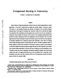
Figure 1. Normal scenes from everyday life are compressible with respect to a basis of wavelets. (left) A test image. (top) One standard compression procedure is to represent the image as a sum of wavelets. Here, the coefficients of the wavelets are plotted, with large coefficients identifying wavelets that make a significant contribution to the image (such as identifying an edge or a texture). (right) When the wavelets with small coefficients are discarded and the image is reconstructed from only the remaining wavelets, it is nearly indistinguishable from the original. (Photos and figure courtesy of Emmanuel Candes.)

116

What’s Happening in the Mathematical Sciences

Even conventional infrared light is expensive to image. “When you move outside the range where silicon is sensitive, your $100 camera becomes a $100,000 camera,” says Baraniuk. In some applications, such as spacecraft, there may not be enough room for a lot of sensors. For applications like these, it makes sense to think seriously about how to make every pixel count.

The Old Conventional Wisdom The story of compressed sensing begins with Claude Shannon, the pioneer of information theory. In 1949, Shannon proved that a time-varying signal with no frequencies higher than N hertz can be perfectly reconstructed by sampling the signal at regular intervals of 1/2N seconds. But it is the converse theorem that became gospel to generations of signal processors: a signal with frequencies higher than N hertz cannot be reconstructed uniquely; there is always a possibility of aliasing (two different signals that have the same samples). In the digital imaging world, a “signal” is an image, and a “sample” of the image is typically a pixel, in other words a measurement of light intensity (perhaps coupled with color information) at a particular point. Shannon’s theorem (also called the Shannon-Nyquist sampling theorem) then says that the resolution of an image is proportional to the number of measurements. If you want to double the resolution, you’d better double the number of pixels. This is exactly the world as seen by digital-camera salesmen. Candes, Tao, Romberg, and Donoho have turned that world upside down. In the compressed-sensing view of the world, the achievable resolution is controlled primarily by the information content of the image. An image with low information content can be reconstructed perfectly from a small number of measurements. Once you have made the requisite number of measurements, it doesn’t help you to add more. If such images were rare or unusual, this news might not be very exciting. But in fact, virtually all real-world images have low information content (as shown in Figure 1). This point may seem extremely counterintuitive because the mathematical meaning of “information” is nearly the opposite of the common-sense meaning. An example of an image with high information content is a picture of random static on a TV screen. Most laymen would probably consider such a signal to contain no information at all! But to a mathematician, it has high information content precisely because it has no pattern; in order to describe the image or distinguish between two such images, you literally have to specify every pixel. By contrast, any real-world scene has low information content because it is possible to convey the content of the image with a small number of descriptors. A few lines are sufficient to convey the idea of a face, and a skilled artist can create a recognizable likeness of any face with a relatively small number of brush strokes.2

Terence Tao. (Photo courtesy of Reed Hutchinson/UCLA.)

2

The modern-day version of the “skilled artist” is an image compression algorithm, such as the JPEG-2000 standard, which reconstructs a copy of the original image from a small number of components called wavelets. (See “Parlez-vous Wavelets?” in What’s Happening in the Mathematical Sciences, Volume 2.) What’s Happening in the Mathematical Sciences

117

Justin Romberg. (Photo courtesy of Justin Romberg.)

The idea of compressed sensing is to use the low information content of most real-life images to circumvent the Shannon-Nyquist sampling theorem. If you have no information at all about the signal or image you are trying to reconstruct, then Shannon’s theorem correctly limits the resolution that you can achieve. But if you know that the image is sparse or compressible, then Shannon’s limits do not apply. Long before “compressed sensing” became a buzzword, there had been hints of this fact. In the late 1970s, seismic engineers started to discover that “the so-called fundamental limits weren’t fundamental,” says Donoho. Seismologists gather information about underground rock formations by bouncing seismic waves off the discontinuities between strata. (Any abrupt change in the rock’s state or composition, such as a layer of oil-bearing rock, will reflect a vibrational wave back to the surface.) In theory the reflected waves did not contain enough information to reconstruct the rock layers uniquely. Nevertheless, seismologists were able to acquire better images than they had a right to expect. The ability to “see underground” made oil prospecting into less of a hit-or-miss proposition. The seismologists explained their good fortune with the “sparse spike train hypothesis,” Donoho says. The hypothesis is that underground rock structures are fairly simple. At most depths, the rock is homogeneous, and so an incoming seismic wave sees nothing at all. Intermittently, the seismic waves encounter a discontinuity in the rock, and they return a sharp spike to the sender. Thus, the signal is a sparse sequence of spikes with long gaps between them. In this circumstance, it is possible to beat the constraints of Shannon’s theorem. It may be easier to think of the dual situation: a sparse wave train that is the superposition of just a few sinusoidal waves, whose frequency does not exceed N hertz. If there are K frequency spikes in a signal with maximal frequency N, Shannon’s theorem would tell you to collect N equally spaced samples. But the sparse wave train hypothesis lets you get by with only 3K samples, or even sometimes just 2K. The trick is to sample at random intervals, not at regular intervals (see Figures 2 and 3). If K