Compression of microarray images

Compression of microarray images

429

22 0 Compression of microarray images * António J. R. Neves and Armando J. Pinho

Signal Processing Lab, DETI/IEETA, University of Aveiro Portugal

1. Introduction DNA microarrays have become a tool of paramount importance in the study of gene function, regulation, and interaction across large numbers of genes, and even entire genomes (Hegde et al., 2000; Moore, 2001). Microarray experiments generate pairs of 16 bits per pixel grayscale images (see Fig. 1, for an example). These images, which may require several tens of megabytes in order to be stored or transmitted, are analyzed by software tools that extract relevant information, such as the intensity of the spots and the background level. This information is then used for evaluating the expression level of individual genes (Hegde et al., 2000; Moore, 2001).

(a) Green channel (b) Red channel Fig. 1. Example of a pair of images (1041 × 1044 pixels) that results from a microarray experiment. The common approach for microarray compression has been based on image analysis for spot finding (griding followed by segmentation) with the aim of separating the microarray image data into different streams based on pixel similarities (Adjeroh et al., 2006; Faramarzpour and Shirani, 2004; Faramarzpour et al., 2003; Hua et al., 2003; 2002; Jörnsten et al., 2003; 2002a; Lonardi and Luo, 2004; Zhang et al., 2005). Once separated, the streams are compressed together with the segmentation information. A potential drawback of these segmentation based * This

work was supported in part by the FCT (Fundação para a Ciência e Tecnologia).

430

Signal Processing

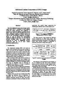
approaches is that different spot placements (e.g., non-rectangular) might compromise their performance. In fact, although initially the rectangular packing was the organization used for spot placement in microarrays, other non-rectangular packings have also been proposed (see Fig. 2).

(a) Rectangular packing (b) Orange packing Fig. 2. Different spot packing: (a) Rectangular packing; (b) Orange packing (sample image from http://microarray1k.aecom.yu.edu/). Note that these images are not related. They serve just for illustrating different spot placements. Although initially most of the specialized techniques for microarray image compression considered the lossy approach as a reasonable possibility (Faramarzpour and Shirani, 2004; Hua et al., 2003; 2002; Jörnsten et al., 2003; 2002a), the most recent methods address mainly reversible techniques (Faramarzpour et al., 2003; Lonardi and Luo, 2004; Zhang et al., 2005). Keeping the original images allows future re-analysis by possibly better algorithms. In fact, the analytic methods that are used for extracting information from the images are continuously being improved (Kothapalli et al., 2002; Leung and Cavalieri, 2003; Sasik et al., 2004). Also, as with other biomedical related data, legal issues might play a key role when choosing between maintaining or deleting the original data. Recently, we have investigated methods for compressing microarray images that do not require spot segmentation. This new approach is based on arithmetic coding that is driven by image-dependent multi-bitplane finite-context models. Basically, the image is compressed on a bitplane basis, going from the most significant to the least significant bitplane. The finitecontext model used by the arithmetic encoder uses (causal) pixels from the bitplane under compression and also pixels from the bitplanes already encoded. To our knowledge, this technique is currently the best one available in terms of compression efficiency of microarray images (Neves and Pinho, 2009). In this chapter, we start by describing the most important techniques for the lossless compression of microarray images that have been proposed in the literature. Then, we present a set of experiments that have been performed with the aim of providing a reference regarding the performance of standard image coding techniques, namely, lossless JPEG2000, JBIG and JPEG-LS, when applied to the lossless compression of microarray images. We proceed with the description of an image-independent multi-bitplane finite-context approach and we continue with the image-dependent version. Finally, we present experimental results that


431

illustrate the compression performance of the several approaches and we draw some conclusions.

2. Compression techniques for microarray images In this section, we present the most important methods for compression of microarray images, namely, the works of Jörnsten et al. (2003), Hua et al. (2002), Faramarzpour et al. (2003), Lonardi and Luo (2004) and Zhang et al. (2005). Although all the methods presented in this section address the microarray compression problem using different approaches, some of the processing steps are common and similar to the ones depicted in Fig. 3. All the methods start by segmenting the microarray images into regions of interest (ROIs) containing the spot and some surrounding background. Some methods go even further, separating the spot area from the background. However, the segmentation algorithm used in each method is different. Microarray image

Gridding

Segmentation

Header coding

Spots coding

Background coding

Compressed image

Fig. 3. The common processing steps of the compression methods presented in this section. Through segmentation, it is possible to encode the spots and background separately. This is explicitly done in the works of Hua et al. (2003; 2002); Jörnsten et al. (2003); Jörnsten and Yu (2000; 2002); Jörnsten et al. (2002a;b); Lonardi and Luo (2004), and more implicilty in the work of Faramarzpour and Shirani (2004); Faramarzpour et al. (2003), because, in this case, the separation between the spot area and the background is performed only when the sequence is entropy encoded. Almost all available methods have also a lossy compression version. These methods remove what is considered to be noise or redundant. Although this step sounds obvious, the question is “What should be considered noise or redundant?” Note that, in the context of microarray images, the background is very important for noise estimation, because the bias due to noise can be estimated and removed in the calculation of the gene expression level of each spot.

432

Signal Processing

The technique proposed by Jörnsten et al. (2003) is characterized by a first stage devoted to griding and segmentation. Using the approximate center of each spot, a seeded region growing is performed for segmenting the spots. The segmentation map is encoded using chain-coding, whereas the interior of the regions are encoded using a modified version of the LOCO-I algorithm (LOw COmplexity LOssless COmpression for Images, the algorithm behind the JPEG-LS coding standard), named SLOCO. Besides lossy-to-lossless capability, Jörnsten’s technique allows partial decoding by means of independently encoded image blocks. Hua et al. (2002) presented a transform-based coding technique. Initially, a segmentation is performed using the Mann-Whitney algorithm and the segmentation information is encoded separately. Due to the thresholding properties of the Mann-Whitney algorithm, the griding stage is avoided. Then, a modified EBCOT (Embedded Block Coding with Optimized Truncation) (Taubman and Marcellin, 2002) for handling arbitrarily shaped regions is used for encoding the spots and background separately, allowing lossy-to-lossless coding of background only (with the spots encoded in lossless mode) or both background and spots. The compression method proposed by Faramarzpour et al. (2003) starts by locating and extracting the microarray spots, isolating each spot into an individual ROI. A spiral path is adjusted to each of these ROIs, such that its center coincides with the center of mass of the spot. The idea is to transform the ROI into an one-dimensional signal with minimum entropy. Then, predictive coding is applied along this path, with a separation between residuals belonging to the spot area and those belonging to the background area. Lonardi and Luo (2004) proposed lossless and lossy compression algorithms for microarray images (MicroZip). The method uses a fully automatic griding procedure, similar to that of Faramarzpour’s method, for separating spots from the background (which can be lossy compressed). Through segmentation, the image is split into two streams: foreground and background. Then, for entropy coding, each stream is divided into two 8 bit sub-streams and arithmetic encoded, with the option of being previously processed by a Burrows-Wheeler transform. The method proposed by Adjeroh et al. (2006); Zhang et al. (2005) is based on PPAM (Prediction by Partial Approximate Matching). PPAM is an image compression algorithm which extends the PPM text compression algorithm, considering the special characteristics of natural images (Zhang et al., 2005). Initially, the microarray image is separated into background and foreground. Then, for each of these two components, the pixel representation is separated into its most significant and least significant parts. To compress the data, the most significant part is first processed by an error prediction scheme. The residuals are then encoded by the PPAM context model and encoder. The least significant part is encoded directly by the PPAM encoder and the segmentation information is saved without compression.

3. Standard image compression methods JBIG, JPEG-LS and JPEG2000 are state-of-the-art standards for coding digital images. They have been developed with different goals in mind, being JBIG more focused on bi-level imagery, JPEG-LS dedicated to the lossless compression of continuous-tone images and JPEG2000 designed with the aim of providing a wide range of functionalities. The JBIG standard (Joint Bi-level Image Experts Group) was issued in 1993 by ISO/IEC (International Organization for Standardization / International Electrotechnical Commission) and ITU-T (Telecommunication Standardization Sector of the International Telecommunication Union) for the progressive lossless compression of binary and low-precision gray-level images (typically, having less than 6 bits per pixel). The major advantages of JBIG over other


433

existing standards, such as FAX Group 3/4, are its capability of progressive encoding and its superior compression efficiency (Hampel et al., 1992; ISO/IEC, 1993; Netravali and Haskell, 1995; Salomon, 2000). The core of JBIG is an adaptive context-based arithmetic encoder, relying on 1024 contexts when operating in sequential mode or on low resolution layers of the progressive mode, or 4096 contexts when encoding high resolution layers. More recently, a new version, named JBIG2, has been published (ISO/IEC, 2000b), introducing additional functionalities to the standard, such as multipage document compression, two modes of progressive compression, lossy compression and differentiated compression methods for different regions of the image (e.g., text or halftones) (Salomon, 2000). JPEG-LS was developed by the Joint Photographic Experts Group (JPEG) with the aim of providing a low complexity lossless image standard that could be able to offer better compression efficiency than lossless JPEG (ISO/IEC, 1999; Taubman and Marcellin, 2002; Weinberger et al., 2000). Part 1 of this standard was finalized in 1999. The core of JPEG-LS is based on the LOCO-I algorithm, that relies on prediction, residual modeling and context-based coding of the residuals. Most of the low complexity of this technique comes from the assumption that prediction residuals follow a two-sided geometric probability distribution and from the use of Golomb codes which are known to be optimal for this kind of distributions. Besides lossless compression, JPEG-LS also provides a lossy mode where the maximum absolute error can be controlled by the encoder. This is known as near-lossless compression or L∞ -constrained compression. From the three image coding standards addressed in this section, JPEG2000 is the most recent one (ISO/IEC, 2000a; Taubman and Marcellin, 2002). Part 1 was published as an International Standard in the year 2000. It is based on wavelet technology and EBCOT coding of the wavelet coefficients, providing very good compression performance for a wide range of bitrates, including lossless coding. Moreover, JPEG2000 allows the generation of embedded code streams, meaning that from a higher bitrate stream it is possible to extract lower bitrate instances without the need for re-encoding. This property is of fundamental importance for progressive transmission, for example, over slow communication channels. These three standard image encoders cover a great variety of coding approaches. In fact, whereas JPEG2000 is transform based, JPEG-LS relies on predictive coding, and JBIG relies on context-based arithmetic coding. This diversity in coding engines might be helpful for drawing conclusions regarding the appropriateness of each of these technologies for the case of microarray image compression. 3.1 Compression performance of the standards

Before trying to develop new compression methods, it is always useful to find out how existing compression standards behave on the class of images of interest. Therefore, for performing that assessment, we collected microarray images from three different publicly available sources: (1) 32 images that we refer to as the Apo AI set and which have been collected from http://www.stat.berkeley.edu/users/terry/zarray/Html/index. html (this set was previously used by Jörnsten et al. (2003); Jörnsten and Yu (2002)); (2) 14 images forming the ISREC set which have been collected from http://www.isrec.isb-sib. ch/DEA/module8/P5_chip_image/images/; (3) three images previously used to test MicroZip (Lonardi and Luo, 2004), which were collected from http://www.cs.ucr.edu/ ~yuluo/MicroZip/.

434

Signal Processing

JBIG compression was obtained using version 1.6 of the JBIG Kit package1 , with sequential coding (-q flag). JPEG2000 lossless compression was obtained using version 5.1 of the JJ2000 codec with default parameters (lossless compression)2 . JPEG-LS coding was obtained using version 2.2 of the SPMG JPEG-LS codec with default parameters3 . For additional reference, we also give compression results using the popular compression tool GZIP (version 1.2.4). Table 1 shows the compression results, in number of bits per pixel (bpp), where the first group of images corresponds to the Apo AI set, the second to the ISREC set and the third one to the MicroZip image set. Image size ranges from 1000 × 1000 to 5496 × 1956 pixels, i.e., from uncompressed sizes of about 2 megabytes to more than 20 megabytes (all images have 16 bits per pixel). The average results presented take into account the different sizes of the images, i.e., they correspond to the total number of bits divided by the total number of image pixels. Image set

Gzip

JPEG2000

APO_AI ISREC Microzip Average

12.711 12.464 11.434 12.273

11.063 11.366 9.515 10.653

JBIG 10.851 10.925 9.297 10.393

JPEG-LS 10.608 11.145 8.974 10.218

Table 1. Compression results, in bits per pixel (bpp), using lossless JPEG2000, JBIG and JPEGLS. For reference, results are also given for the popular compression tool GZIP. The total average results show that gains of about 13.2%, 15.3% and 16.7%, in relation to GZIP compression, are attained respectively for lossless JPEG2000, JBIG and JPEG-LS, showing the superiority of image coding techniques over general purpose data compression methods in the task of compressing images. The average results by image set show that JPEG-LS provides the highest compression in the case of the Apo AI and MicroZip images, whereas JBIG gives the best results for the ISREC set. Lossless JPEG2000 is always slightly behind these two. It is interesting to note that the set for which JBIG gave the best results is also the one requiring more bits per pixel for encoding. 3.1.1 Sensitivity to noise

It has been noted by Jörnsten et al. (2003) that, in general, the eight least significant bitplanes of cDNA microarray images are close to random and, therefore, incompressible. Since this fact may result in some degradation in the compression performance of the encoders, we decided to address this problem and to study the effect of noisy bitplanes in the compression performance of the standards. To perform this evaluation, we separated the images into a number p of most significant bitplanes and 16 − p least significant bitplanes. Whereas the p most significant bitplanes have been sent to the encoder, the 16 − p least significant bitplanes have been left uncompressed. This means that the bitrate of a given image is the sum of the bitrate generated by encoding the p most significant bitplanes plus the 16 − p bits concerning the bitplanes that have been left uncompressed. 1 2 3

http://www.cl.cam.ac.uk/~mgk25/jbigkit/. http://jj2000.epfl.ch. The original website of this codec, http://spmg.ece.ubc.ca, is currently unavailable. However, it can be obtained from ftp://www.ieeta.pt/~ap/codecs/jpeg_ls_v2.2.tar.gz.


435

15

JBIG: 1230c1G JPEG-LS: 1230c1G JPEG2000: 1230c1G

Bitrate (bpp)

14

13

12

11

10 2

4

6 8 10 12 Number of bitplanes encoded

15

14

16

14

16

JBIG: array1 JPEG-LS: array1 JPEG2000: array1

Bitrate (bpp)

14

13

12

11

10 2

4

6 8 10 12 Number of bitplanes encoded

Fig. 4. Influence of noisy bitplanes in the performance of the standard encoding methods. The the curves indicate the bitrate obtained when only a given number p of the most significant bitplanes are sent to the encoder, whereas the other 16 − p bitplanes are left uncompressed. Image set Apo_AI ISREC MicroZip Average

JPEG2000 8 bp Best 10.940 10.790 11.100 10.954 9.918 9.321 10.661 10.376

JBIG 8 bp Best 10.510 10.507 10.607 10.583 9.506 9.030 10.224 10.073

JPEG-LS 8 bp Best 10.523 10.433 10.838 10.713 9.588 8.912 10.302 10.026

Table 2. Average compression results, in bits per pixel (bpp), when a number of bitplanes is left uncompressed. The columns labeled “8 bp” provide results for the case where only the 8 most significant bitplanes have been encoded and the 8 least significant bitplanes have been left uncompressed. The column named “Best” contains the results for the case where the separation of most and least significant bitplanes has been optimally found.

436

Signal Processing

Figure 4 depicts bitrate curves, as a function of p, for two different images, “1230c1G” and “array1”. As can be observed, the best bitrate is generally not met when compressing all 16 bitplanes, but instead when some of the least significant bitplanes are left uncompressed. However, the value of the optimum value of p, popt , varies not only from image to image, but also from one encoder to the other. In fact, for the Apo AI set, which is characterized by the most regular value of popt , JBIG is the encoder with the highest value of popt (around 8), then comes lossless JPEG2000 (around 10) and, finally, JPEG-LS (around 13). This result is not surprising, since JBIG encodes the bitplanes independently. Therefore, without being able to get information from other bitplanes, it is natural that JBIG starts considering bitplanes as “noise” earlier than the other encoders. Moreover, this can also be the justification for its better performance in the ISREC set, because it is the most noisy. Table 2 compares average results for the three set of images regarding two situations: (1) the image is divided into the eight most significant bitplanes (which are encoded) and the eight least significant bitplanes (which are left uncompressed); (2) the optimum value of p is determined for each image. From this table, and comparing with the Table 1, we can see that, in fact, this splitting operation can provide some additional compression gains. The best results attained provided improvements of 3.1%, 2.6% and 1.9% respectively for JBIG, lossless JPEG2000 and JPEG-LS. However, finding the right value for p may require as many as 16 iterations of the compression phase in order to find it. Moreover, from the results shown in Table 2, we can see that a simple separation of the bitplanes in an upper and lower half may improve the compression in some cases (Apo AI and ISREC image sets), but may also produce the opposite result (MicroZip image set). 3.1.2 Lossy-to-lossless compression

From the point of view of compression efficiency, and taking into account the results presented in Table 1, JPEG-LS is the overall best lossless compression method, followed by JBIG and lossless JPEG2000. The difference between JPEG-LS and lossless JPEG2000 is about 4.1% and between JPEG-LS and JBIG is only 1.7%. However, the better compression performance provided by JPEG-LS can be overshadowed by a potentially important functionality provided by the other two standards, which is progressive, lossy-to-lossless, transmission. In the case of lossless JPEG2000, this functionality is basically a by-product of the multiresolution wavelet technology used in its encoding engine and also due to a strategy of encoding the information in layers (Taubman and Marcellin, 2002). In the case of JBIG, this property comes from two different sources. On one hand, images with more that one bitplane are encoded using a bitplane-by-bitplane coding approach. This provides a kind of progressive transmission, from most to least significant bitplanes, where the precision of the pixels is improved for each added bitplane. Moreover, this technique produces a reduction of the L∞ error by a factor of two for each additional bitplane. On the other hand, JBIG permits the progressive transmission of each bitplane by progressively increasing its spatial resolution (ISO/IEC, 1993; Salomon, 2000). However, the compression results that we present in Table 1 do not take into account the additional overhead implied by this encoding mode of JBIG (we used the -q flag of the encoder, which disables this mode). In Fig. 5, we present rate-distortion curves for two images, “1230c1G” and “array1”, obtained with the lossless JPEG2000 and JBIG coding standards, and according to two error metrics: L2 -norm (root mean squared error) and L∞ -norm (maximum absolute error). Regarding the L2 -norm, we observe that lossless JPEG2000 provides slightly better rate-distortion results for

Root mean squared error


10

4

10

3

JBIG: 1230c1G JPEG2000: 1230c1G JBIG: array1 JPEG2000: array1

102

10

1

0.1

10 Maximum absolute error

437

0

2

4 6 8 Bitrate (bpp)

10

12

5

JBIG: 1230c1G JPEG2000: 1230c1G JBIG: array1 JPEG2000: array1

104 103

10

2

10

1

0

2

4 6 8 Bitrate (bpp)

10

12

Fig. 5. Rate distortion curves showing the performance of lossless JPEG2000 and JBIG in a lossy-to-lossless mode of operation. Results are given both for the L2 (root mean squared error) and L∞ (maximum absolute error) norms. bitrates less than 8 bpp. For higher bitrates, this codec exhibits a sudden degradation of the rate-distortion. We believe that this phenomenon is related to the default parameters used by the encoder, which might not be well suited for images having 16 bits per pixel, such as those of the microarrays. Moreover, we think that a careful setting of these parameters may lead to improvements in the rate-distortion of JPEG2000 for bitrates higher than 8 bpp, although we consider this tuning a problem that is beyond the scope of this work. With respect to the L∞ -norm, we observe that JBIG is the one with the best rate-distortion performance. In fact, due to its bitplane-by-bitplane approach, it guarantees an exponential and upper bounded decrease of the maximum absolute error. The upper bound of the error is given by 2(16− p) − 1, where p is the number of bitplanes already decoded. Contrarily, lossless JPEG2000 cannot guarantee such bound, which may be a major drawback in some cases. Finally, we note that the sudden deviation of the lossless JPEG2000 curves around bitrates of 8 bpp is probably related to the same problem pointed out earlier for the case of the L2 -norm.

438

Signal Processing

3.2 Conclusions

The main objective of this section was to provide a set of comprehensive results regarding the lossless compression of microarray images by state-of-the-art image coding standards, namely, lossless JPEG2000, JBIG and JPEG-LS. In order to facilitate future comparisons by other researchers, we collected a total of 49 microarray images available from the Internet. We believe that the development of specialized compression techniques should be supported by a preliminary study of the performance provided by well established methods and, particularly, by those that are standards. Only after making such study it is possible to be in a comfortable position for arguing about the relevance of some specialized technique. From the experimental results obtained, we conclude that JPEG-LS gives the best lossless compression performance. However, it lacks lossy-to-lossless capability, which may be a decisive functionality if remote transmission over possibly slow links is a requirement. Complying to this requirement we find JBIG and lossless JPEG2000, lossless JPEG2000 being the best considering rate-distortion in the sense of the L2 -norm and JBIG the most efficient when considering the L∞ -norm. Moreover, JBIG is consistently better than lossless JPEG2000 regarding lossless compression ratios. Also, JBIG is the method that can benefit most from a correct separation of most significant bitplanes that are encoded and least significant bitplanes that are left uncompressed (it gained 3.1%), and it is also the coding technique that, due to the bitplaneby-bitplane coding, can search for the optimum point of separation on-the-fly. In fact, this can be done by monitoring the bitrate resulting from the compression of each bitplane, and stop doing compression when this value is over 1 bpp. As a final conclusion, and according to what we presented in this section, it is our opinion that the technology behind JBIG seems to be the most appropriate for microarray image coding.

4. Compression of microarray images using finite-context models and arithmetic coding 4.1 Finite-context models

The core of the methods proposed in the remainder of this chapter consists of an adaptive finite-context model followed by arithmetic coding. A finite-context model (see Fig. 6) of an information source assigns probability estimates to the symbols of an alphabet A, according to a conditioning context computed over a finite and fixed number, M, of past outcomes (orderM finite-context model) (Rissanen, 1983; Rissanen and Langdon, Jr., 1981; Sayood, 2000). At time t, we represent these conditioning outcomes by ct = xt− M+1 , . . . , xt−1 , xt . The number of conditioning states of the model is |A| M , dictating its complexity (or model cost). In our case, A = {0, 1} and, therefore, |A| = 2. In practice, the probability that the next outcome, xt+1 , is “0” is obtained using the estimator P ( x t +1 = 0| c t ) =

n(0, ct ) + δ n(0, ct ) + n(1, ct ) + 2δ

,

(1)

where n(s, ct ) represents the number of times that, in the past, the information source generated symbol s ∈ A having ct as the conditioning context. The parameter δ > 0, besides allowing fine tuning the estimator, avoids generating zero probabilities when a symbol is encoded for the first time. In our case, we used δ = 1, which corresponds to Laplace’s estimator (it can be seen as an initialization of all counters to one). The counters are updated each time a symbol is encoded. Since the context template is causal, the decoder is able to reproduce the same probability estimates without needing additional information.


...

439

x t−4

x t+1

0 1 0 1 0 1 0 0 1 1 0

...

Context ct Model

Input symbol

P(xt+1= s | c t ) Encoder

Output bit−stream

Fig. 6. Finite-context model: the probability of the next outcome, xt+1 , is conditioned by the M last outcomes. In this example, M = 5. Context, ct 00000 00001 00010 00011 00100 .. . 11111

n(0, ct ) 23 16 19 34 36 .. . 8

n(1, ct ) 41 6 30 42 17 .. . 2

n(0, ct ) + n(1, ct ) 64 22 49 76 53 .. . 10

Table 3. Simple example illustrating how finite-context models are implemented. The rows of the table represent a probability model at a given instant t. In this example, the particular model that is chosen for encoding a symbol depends on the last five encoded symbols (order-5 context). Table 3 shows an example of how a finite-context is typically implemented. In this example, an order-5 finite-context model is presented. Each row represents a probability model that is used to encode a given symbol according to the last encoded symbols (five in this example). Therefore, if the last symbols were “00010”, i.e., ct = 00010, then the model communicates the following probability estimates to the arithmetic encoder: P(0|00010) = 19/49 and P(1|00010) = 30/49. The block denoted “Encoder” in Fig. 6 is an arithmetic encoder. It is well known that practical arithmetic coding generates output bit-streams with average bitrates almost identical to the entropy of the model (Bell et al., 1990; Salomon, 2000; Sayood, 2000). In our case, the theoretical bitrate average (entropy) of the model after encoding N symbols is given by HN = −

1 N −1 log2 P( xt+1 = s|ct ) N t∑ =0

bps,

(2)

where “bps” stands for “bits per symbol”. Since we are dealing with images, instead of using the generic “bps” measure we use “bpp”, which stands for “bits per pixel”. Recall that the

440

Signal Processing

entropy of any sequence of two symbols is limited to 1 bps, a value that is achieved when the symbols are independent and equally likely. 4.2 Image-independent contexts

In Section 3, we presented a study of the compression performance of three image coding standards in the context of microarray image compression: JPEG2000, JBIG and JPEG-LS. Since they rely on three different coding technologies, we were able not only to evaluate the performance of each of these standards, but also to collect hints regarding what might be the best coding technology regarding microarray image compression. In that study, we concluded that from the three technologies evaluated (predictive coding in the case of JPEG-LS, transform coding in the case of JPEG2000 and context-based arithmetic coding in the case of JBIG), the technology behind JBIG seemed to be the most promising. In fact, JPEG-LS provided the highest compression, closely followed by JBIG. However, unlike JPEG2000 and JBIG, it does not provide lossy-to-lossless capabilities, a characteristic that might be of high interest, specially in the case where remote databases have to be accessed using transmission channels of reduced bandwidth. Moreover, with JBIG, the image bitplanes are compressed independently, suggesting the existence of some room for improvement. Motivated by these observations, we developed a compression method for microarray images which is based on the same technology as JBIG but that, unlike JBIG, exploits inter-bitplane dependencies, providing coding gains in relation to JBIG (Neves and Pinho, 2006). Designing contexts that gather information from more than one bitplane (multi-bitplane contexts) is not just a matter of joining more bits to the context, because for each new bit added the memory required doubles. Moreover, there is the danger of running into the context dilution problem, due to the lack of sufficient data for estimating the probabilities. Therefore, this extension to multi-bitplane contexts must be done carefully. The method proposed by Neves and Pinho (2006) was inspired by EIDAC (Yoo et al., 1998), a compression method that has been used with success for coding images with a reduced number of intensities (simple images). The images are compressed on a bitplane basis, from the most to the least significant bitplane. The causal finite-context model that drives the arithmetic encoder uses pixels both from the bitplane currently being encoded and from the bitplanes already encoded. As encoding proceeds, the average bitrate obtained after encoding each bitplane is monitored. If, for some bitplane, the average bitrate exceeds one bit per pixel, then the encoding process is stopped and the remaining bitplanes are saved without compression. The encoding procedure is outlined in Fig. 7. The context modeling part of EIDAC was designed mainly with the aim of compressing images with eight bitplanes or less, implying, at most, 19 bits of context. A straightforward extension to images with 16 bitplanes would require contexts of 27 bits, i.e., at least 2 × 227 = 228 counters. Essentially, the technique proposed by Neves and Pinho (2006) differs from EIDAC in three aspects: (1) it was designed taking into account the specific nature of the images, keeping the size of the contexts limited to 21 bits; (2) it does not use the histogram packing procedure proposed for EIDAC because, generally, microarray images have dense intensity histograms; (3) it implements a rate-control mechanism that avoids producing average bitrates of more than one bit per pixel in bitplanes that are too noisy (this is a common characteristic of the least significant bitplanes of microarray images (Jörnsten et al., 2003)). As we mentioned before, choosing the context template for a multi-bitplane image is a critical task, requiring tradeoffs involving aspects such as the maximum size of the context, the problem of context dilution and the placement of the context bits such that the maximum informa-


441

Input Image Encode bitplane k k = 15, 14, 13, ..., 0 Choose the best context size Encode all pixels in the bitplane

Bitrate > 1bpp

No

Yes Save the remaining bitplanes uncompressed Fig. 7. Encoding procedure of the method proposed by Neves and Pinho (2006). The choice of the context shape is based on Fig. 8. Note that, being a bitplane based encoder, it is possible to monitor the bitrate used to encode each bitplane. tion can be collected. This work was done in (Neves and Pinho, 2006) mainly using a trial and error procedure, leading to the image-independent context configuration displayed in Fig. 8. Note that, when encoding the eight least significant bitplanes, the finite-context model is only formed with pixels from the higher numbered bitplanes. This specific context configuration together with the rate-control mechanism avoids the degradation in compression rate when there are bitplanes that are close to random and, therefore, are almost incompressible. Although being able to provide state-of-the-art compression results, the method proposed in (Neves and Pinho, 2006) could be improved. In fact, due to its image-independent nature, and despite being designed for a specific type of images (microarrays), the context configuration depicted in Fig. 8 resulted from a complicated process that tried to balance the inevitable particularities among the images. From the point of view of a single image, this context configuration might seem overkill, i.e., a smaller context might suffice. However, it is needed for satisfying the ensemble of images. This observation motivated the image-dependent contextmodeling approach that we describe in the next section.

442

Signal Processing

? (a) BP = 15

? (b) BP = 14 ? (c) BP = 13 ? (d) 8