Compressive Wavefront Sensing with Weak Values Gregory A. Howland,1,∗ Daniel J. Lum1 , and John C. Howell1
arXiv:1405.3671v1 [physics.optics] 14 May 2014
1 University
of Rochester Department of Physics and Astronomy, 500 Wilson Blvd, Rochester, NY 14618, USA *
[email protected]
Abstract: We demonstrate a wavefront sensor based on the compressive sensing, single-pixel camera. Using a high-resolution spatial light modulator (SLM) as a variable waveplate, we weakly couple an optical field’s transverse-position and polarization degrees of freedom. By placing random, binary patterns on the SLM, polarization serves as a meter for directly measuring random projections of the real and imaginary components of the wavefront. Compressive sensing techniques can then recover the wavefront. We acquire high quality, 256 × 256 pixel images of the wavefront from only 10, 000 projections. Photon-counting detectors give sub-picowatt sensitivity. © 2014 Optical Society of America OCIS codes: (110.1758) Computational imaging, (270.0270) Quantum optics, (010.1080) Active or adaptive optics, (120.5050) Phase measurement
References and links 1. F. Roddier, Adaptive optics in astronomy (Cambridge university press, 1999). 2. L. N. Thibos and X. Hong, “Clinical applications of the Shack-Hartmann aberrometer,” Optometry & Vision Science 76, 817–825 (1999). 3. M. J. Booth, “Adaptive optics in microscopy,” Philosophical Transactions of the Royal Society A: Mathematical, Physical and Engineering Sciences 365, 2829–2843 (2007). 4. M. Levoy, “Light fields and computational imaging,” IEEE Computer 39, 46–55 (2006). 5. R. Tyson, Principles of adaptive optics (CRC Press, 2010). 6. J. S. Lundeen, B. Sutherland, A. Patel, C. Stewart, and C. Bamber, “Direct measurement of the quantum wavefunction,” Nature 474, 188–191 (2011). 7. B. C. Platt and R. Shack, “History and principles of Shack-Hartmann wavefront sensing,” Journal of Refractive Surgery 17, S573–S577 (2001). 8. R. Lane and M. Tallon, “Wave-front reconstruction using a Shack-Hartmann sensor,” Applied optics 31, 6902– 6908 (1992). 9. S. Kocsis, B. Braverman, S. Ravets, M. J. Stevens, R. P. Mirin, L. K. Shalm, and A. M. Steinberg, “Observing the average trajectories of single photons in a two-slit interferometer,” Science 332, 1170–1173 (2011). 10. J. Z. Salvail, M. Agnew, A. S. Johnson, E. Bolduc, J. Leach, and R. W. Boyd, “Full characterization of polarization states of light via direct measurement,” Nature Photonics 7, 316–321 (2013). 11. D. Takhar, J. N. Laska, M. B. Wakin, M. F. Duarte, D. Baron, S. Sarvotham, K. F. Kelly, and R. G. Baraniuk, “A new compressive imaging camera architecture using optical-domain compression,” in “Electronic Imaging 2006,” (International Society for Optics and Photonics, 2006), pp. 606509–606509. 12. R. G. Baraniuk, “Single-pixel imaging via compressive sampling,” IEEE Signal Processing Magazine (2008). 13. Y. Aharonov, D. Z. Albert, and L. Vaidman, “How the result of a measurement of a component of the spin of a spin-1/2 particle can turn out to be 100,” Physical review letters 60, 1351 (1988). 14. O. Hosten and P. Kwiat, “Observation of the spin hall effect of light via weak measurements,” Science 319, 787–790 (2008). 15. P. B. Dixon, D. J. Starling, A. N. Jordan, and J. C. Howell, “Ultrasensitive beam deflection measurement via interferometric weak value amplification,” Physical review letters 102, 173601 (2009).
16. A. N. Jordan, J. Mart´ınez-Rinc´on, and J. C. Howell, “Technical advantages for weak-value amplification: When less is more,” Phys. Rev. X 4, 011031 (2014). 17. J. Lundeen and A. Steinberg, “Experimental joint weak measurement on a photon pair as a probe of hardys paradox,” Physical review letters 102, 020404 (2009). 18. J. Dressel and A. Jordan, “Significance of the imaginary part of the weak value,” Physical Review A 85, 012107 (2012). 19. J. Dressel, M. Malik, F. M. Miatto, A. N. Jordan, and R. W. Boyd, “Understanding quantum weak values: Basics and applications,” arXiv preprint arXiv:1305.7154 (2013). 20. D. L. Donoho, “Compressed sensing,” Information Theory, IEEE Transactions on 52, 1289–1306 (2006). 21. E. J. Candes, “The restricted isometry property and its implications for compressed sensing,” Comptes Rendus Mathematique 346, 589–592 (2008). 22. A. Chambolle and P.-L. Lions, “Image recovery via total variation minimization and related problems,” Numerische Mathematik 76, 167–188 (1997). 23. E. J. Candes and T. Tao, “Near-optimal signal recovery from random projections: Universal encoding strategies?” Information Theory, IEEE Transactions on 52, 5406–5425 (2006). 24. M. Lustig, D. Donoho, and J. M. Pauly, “Sparse MRI: The application of compressed sensing for rapid MR imaging,” Magnetic resonance in medicine 58, 1182–1195 (2007). 25. J. Bobin, J.-L. Starck, and R. Ottensamer, “Compressed sensing in astronomy,” Selected Topics in Signal Processing, IEEE Journal of 2, 718–726 (2008). 26. D. Gross, Y.-K. Liu, S. T. Flammia, S. Becker, and J. Eisert, “Quantum state tomography via compressed sensing,” Physical review letters 105, 150401 (2010). 27. G. A. Howland and J. C. Howell, “Efficient high-dimensional entanglement imaging with a compressive-sensing double-pixel camera,” Physical Review X 3, 011013 (2013). 28. E. J. Cand`es and M. B. Wakin, “An introduction to compressive sampling,” Signal Processing Magazine, IEEE 25, 21–30 (2008). 29. J. Romberg, “Imaging via compressive sampling [introduction to compressive sampling and recovery via convex programming],” IEEE Signal Processing Magazine 25, 14–20 (2008). 30. C. Li, “Compressive sensing for 3D data processing tasks: applications, models and algorithms,” Ph.D. thesis, Rice University (2011). 31. C. Li, W. Yin, and Y. Zhang, “Users guide for TVAL3: TV minimization by augmented lagrangian and alternating direction algorithms,” CAAM Report (2009). 32. M. A. Figueiredo, R. D. Nowak, and S. J. Wright, “Gradient projection for sparse reconstruction: Application to compressed sensing and other inverse problems,” Selected Topics in Signal Processing, IEEE Journal of 1, 586–597 (2007). 33. G. A. Howland, D. J. Lum, M. R. Ware, and J. C. Howell, “Photon counting compressive depth mapping,” Optics express 21, 23822–23837 (2013). 34. J. D. Hunter, “Matplotlib: A 2D graphics environment,” Computing In Science & Engineering 9, 90–95 (2007).
1.
Introduction
High resolution wavefront sensing is extremely desirable for diverse applications in research and industry. Applications include measuring atmospheric distortion for astronomy or communication [1], opthalmology [2], microscopy [3], light field imaging [4], and adaptive optics [5]. Fundamentally, a wavefront measurement can be equated with measuring the quantum wavefunction [6]. The most common wavefront sensor is the Shack-Hartmann sensor [7, 8], where a highresolution CCD is placed in the focal plane of a lenslet array. The optical power passing through each lenslet gives a local intensity, while the displacement of each lenslet’s focal point on the CCD gives a local phase tilt. Due to the uncertainty principle, Shack-Hartmann sensors are bandwidth-limited; increased spatial resolution comes at the cost of phase precision. A typical Shack-Hartmann sensor might have a spatial resolution of only 30 × 30 lenslets. Recently, Lundeen et. al. used weak measurement to directly measure the transverse wavefunction of a photonic ensemble [6]. By raster scanning a sliver of waveplate through the field, they weakly couple the field’s transverse-position and polarization degrees-of-freedom. After post-selecting on the zero-frequency component of the transverse momentum, the real and imaginary parts of the optical field at the waveplate location are recovered by measuring the final polarization. The measurement is direct; detector values are directly proportional to the real
or imaginary parts of the signal. Similar experiments have used weak measurement to trace the average trajectories of photons in the double slit experiment [9] and to measure the polarization state of a qubit [10]. The technique of Lundeen et. al. is interesting because it has no inherent resolution limitation. However, their measurement process is very inefficient and difficult to scale to high spatial resolution. It requires a slow, physical raster scan of the piece of waveplate through the detection plane. Because the polarization rotation is small, long acquisition times are needed for sufficient signal-to-noise ratio, particularly at low light levels. These limitations make such a system impractical for many applications. To solve these issues, we present a high resolution wavefront sensor that combines Lundeen et. al.’s technique with the compressive sensing (CS) single-pixel camera [11, 12]. In the usual single-pixel camera, a digital micro-mirror device (DMD) is used in conjunction with a single-element detector to take random, linear projections of an intensity image. Optimization techniques are used to recover the image from many fewer projections than pixels in the image. For a wavefront measurement, we replace the DMD with a twisted-nematic (TN) liquid crystal spatial light modulator (SLM). Each SLM pixel acts as an independent, variable waveplate, allowing us to couple transverse-position and polarization without cumbersome scanning. By placing random, binary patterns on the SLM, we directly measure random projections of the real and imaginary parts of the transverse field at high resolution. The real and imaginary parts of the field are recovered with standard, compressive sensing algorithms. We efficiently measure optical wavefronts at up to 256 × 256 pixel resolution. Photoncounting detectors provide extreme low light sensitivity, with typical detected optical power around 0.5 pW. Our system is compact and made of affordable, off-the-shelf components. Like the standard single-pixel camera for intensity imaging, our system can be easily adapted to any wavelength where single-element detectors can be manufactured. 2. 2.1.
Theory Weak Measurement
The weak value, originally presented by Aharonov, Albert, and Vaidman as a “new kind of value for a quantum variable” [13], arises from averaging weak measurements on pre- and post-selected systems. Originally a theoretical curiosity, weak measurement has seen resurgent interest as it has turned out to be very useful, particularly for precision measurement [14–16] and investigation of fundamental phenomena, such as Hardy’s paradox [17]. In a weak measurement, a system of interest is investigated by very weakly coupling it to a measuring device. The system is first prepared in an initial state | ψi. An observable of interest Aˆ is then coupled to an ancillary meter system by a weak interaction or perturbation. Finally, the system is post-selected (projected) into final state | f i. The weak measurement is read-out by a measuring device for the meter. In the limit of a very weak interaction, the measuring device’s pointer is shifted by the weak value Aw =
h f | Aˆ | ψi . h f | ψi
(1)
Note that Aw can be complex valued. The real part of Aw is interpreted as a shift in the pointer’s position; the imaginary part of Aw is interpreted as a shift in the pointer’s momentum [18]. Because the meter’s position and momentum are observables, this enables direct measurement of complex values. For an introduction to experimental weak measurement and weak values, see Refs. [16, 19].
(a)
(b)
(c)
Fig. 1. Weak Value Wavefront Sensing on the Bloch Sphere: A state with transverse field ψ(~x) is initially in polarization | pi i. At ~x = x~0 , the polarization is rotated by small angle θ in the (iˆ, jˆ) plane to state | p f i; this weakly measures ψ(~ x0 ). Following a post selection on transverse momentum ~k = k~0 , the real and imaginary parts of ψ(~ x0 ) are mapped to a polarization rotation of the post-selected state | ψ ps i. The real part generates a rotation αR ˆ jˆ) plane (c). in the (iˆ, jˆ) plane (b) and the imaginary part generates a rotation αI in the (k, The weak measurement of ψ(~ x0 ) is read-out by measuring hσˆ j i and hσˆ k i respectively.
2.2.
Wavefront Sensing with Weak Values
We wish to use weak measurement to directly measure an optical field ψ(~x), where~x = (x, y) are transverse spatial coordinates. In keeping with traditional presentation of weak measurement, we use a quantum formalism where ψ(~x) is treated as a probability amplitude distribution and polarization is represented on the Bloch sphere. Note that the system can still be understood classically, replacing the wavefunction with the transverse electric field and Bloch sphere with the Poincar´e sphere respectively. Consider a weak measurement of position at ~x = x~0 followed by a post-selection of momen˜ ~k) are Fourier transform pairs. The corresponding weak value tum ~k = k~0 , where ψ(~x) and ψ( is hk~0 | x~0 ih~ x0 | ψi eik0 x0 ψ(~ x0 ) Aw (~ x0 ) = = . (2) ˜ k~0 ) hk~0 | ψi ψ( Aw (~ x0 ) is directly proportional to value of the field at position ~x = x~0 up to a linear phase. To obtain Aw (~ x0 ), the field at ~x = x~0 must be weakly coupled to a meter system. The polarization degree of freedom is a convenient meter because it can be easily manipulated and measured. Let ψ(~x) be initially polarized in polarization state | pi i. The full initial state is | ψi =
Z
~ dxψ(~ x) |~xi | pi i.
(3)
At location ~x = x~0 , the polarization is changed from | pi i to a nearby polarization | p f i (Fig. 1a-b). At location x~0 , the state is ψ(~ x0 ) | x~0 i | p f i = ψ(~ x0 )e−iσˆk θ /2 | x~0 i | pi i,
(4)
where the transformation from | pi i to | p f i is expressed as a rotation on the Bloch sphere ˆ This is visualized on the Bloch sphere in Fig. 1. Unit vectors by angle θ about unit vector k.
iˆ, jˆ, and kˆ form a right handed coordinate system on the Bloch sphere, where iˆ points along | pi i, jˆ is the orthogonal unit vector in the plane defined by | pi i and | p f i, and kˆ = iˆ × jˆ (Fig. 1a-c). These unit vectors have corresponding Pauli operators σˆ i , σˆ j , and σˆ k . Note that such a coordinate system can be defined for any two polarization states | pi i and | p f i. For a weak interaction, θ is small. A first order expansion at x~0 yields ψ(~ x0 ) | x~0 i | p f i = ψ(~ x0 )(1 − iσˆk θ /2) | x~0 i | pi i.
(5)
The full state is therefore | ψi =
Z
~ dxψ(~ x) |~xi | pi i − ψ(~ x0 )iσˆk θ /2 | x~0 i | pi i.
(6)
Consider post-selection on a single transverse-momentum~k = k~0 . The post-selected state | ψ ps i no longer has position dependence and is given by ~ ˜ k~0 ) | pi i − ek0 ·~x0 ψ(~ | ψ ps i = hk~0 | ψi = ψ( x0 )iσˆk θ /2 | pi i,
(7)
˜ ~k) is the Fourier transform of ψ(~x). where ψ( ˜ k~0 ) and re-exponentiating, we find Factoring out ψ( ~
−ieik0 ·~x0
˜ k~0 )e | ψ ps i = ψ(
ψ(~ x0 ) σˆ θ ˜ k~0 ) k 2ψ(
˜ k~0 )e−iAw (~x0 )σˆk θ /2 | pi i | pi i = ψ(
(8)
The post-selected polarization state is simply a rotated version of the initial polarization, where the rotation is proportional to ψ(~ x0 ) (Fig. 1a-c). The real part of ψ(~ x0 ) generates a rotation αR in the iˆ, jˆ plane (Fig. 1b). The imaginary part of ψ(~ x0 ) generates a rotation αI in the iˆ, kˆ plane (Fig. 1c). The values are therefore measured by taking expected values of Pauli operators σˆ j and σˆk hψ ps | σˆ j | ψ ps i ∝ Re{ψ(~ x0 )} ps ˆ ps hψ | σk | ψ i ∝ Im{ψ(~ x0 )}. 2.3.
(9) (10)
Random Projections of the Wavefront
Rather than only measuring the wavefunction at a single location ψ(~x = x~0 ), consider instead a weak measurement of an operator fˆi which takes a random, binary projection of ψ(~x), where | fi i is Z | fi i =
d~x fi (~x) | ~xi i.
(11)
The filter function fi (~x) consists of a pixelized, random binary pattern, where pixels in the pattern take on values of 1 or -1 with equal probability. The weak measurement of fˆi , given initial state ψ(~x) and post-selected state | k~0 i, is therefore Ai =
hk~0 | fi ih fi | ψi hk~0 | fi iYi = , ˜ k~0 ) hk~0 | ψi ψ(
(12)
where Yi is the inner product between ψ(~x) and fi (~x) Z
Yi =
d~x fi (~x)ψ(~x).
It is convenient to choose k~0 = (0, 0) to discard the linear phase factor hk~0 | fi i in Eq. 12.
(13)
To perform the weak measurement, we again couple transverse-position to polarization. Unlike the previous case, all of ψ(~x) will now receive a small polarization rotation about kˆ of angle θ for fi (~x) = 1 and −θ for fi (~x) = −1;. Performing an identical derivation to section 2.2, we find a post-selected polarization state ˜ k~0 )e | ψips i = ψ(
−i
Yi ˆ ~ σk θ 2ψ(k0)
| pi i.
(14)
The effective polarization rotation is now proportional to the projection of ψ(~x) onto fi (~x), Yi . Again, taking expectation values of σˆ j and σˆ k yields the real and imaginary parts of Yi , hψips | σˆ j | ψips i ∝ YiRe hψips
| σˆ k | ψips i ∝ YiIm .
(15) (16)
Therefore, weak measurement allows us to directly measure random, binary projections of a transverse field ψ(~x). 2.4.
Compressive Sensing
The random, binary projections of section 2.3 are the type of measurements used in Compressive Sensing [20]. Compressive sensing is a measurement technique that compresses a signal during measurement, rather than after, to dramatically decrease the requisite number of measurements. In compressive sensing, one seeks to recover a compressible, N-dimensional signal X from M