13, No. 4 (2002) 437-453. 437. Computation of dynamic stiffness and flexibility for arbitrarily shaped two-dimensional membranes. J. T. Chenâ and I. L. Chungâ¡.
Structural Engineering and Mechanics, Vol. 13, No. 4 (2002) 437-453
437
Computation of dynamic stiffness and flexibility for arbitrarily shaped two-dimensional membranes J. T. Chen† and I. L. Chung‡ Department of Harbor and River Engineering, National Taiwan Ocean University, Keelung, Taiwan
Abstract. In this paper, dynamic stiffness and flexibility for circular membranes are analytically derived using an efficient mixed-part dual boundary element method (BEM). We employ three approaches, the complex-valued BEM, the real-part and imaginary-part BEM, to determine the dynamic stiffness and flexibility. In the analytical formulation, the continuous system for a circular membrane is transformed into a discrete system with a circulant matrix. Based on the properties of the circulant, the analytical solutions for the dynamic stiffness and flexibility are derived. In deriving the stiffness and flexibility, the spurious resonance is cancelled out. Numerical aspects are discussed and emphasized. The problem of numerical instability due to division by zero is avoided by choosing additional constraints from the information of real and imaginary parts in the dual formulation. For the overdetermined system, the least squares method is considered to determine the dynamic stiffness and flexibility. A general purpose program has been developed to test several examples including circular and square cases. Key words: dynamic stiffness and flexibility; an efficient mixed-part dual BEM; overdetermined system.
1. Introduction Stiffness and flexibility matrices play important roles in structrual analysis (Hibbeler 1997). This concept is easily extended to dynamic stiffness and flexibility if harmonic response is considered (Clough and Penzien 1975). Many approaches including analytical method, finite element method (FEM) and boundary element method (BEM), are considered to determine the stiffness and flexibility. Various analytical dynamic stiffnesses for simple structures were found in the textbook of structural dynamics. In FEM, Paz and Lam (1973, 1975), derived the closed-form solution for general stiffness matrix of a Bernouli-Euler beam and extended the solution to a series form. It is interesting to note that the procedure in deriving stiffness by Mario and Lam is contrary to the derivation by using the multiple reciprocity method (MRM) (Chang et al. 1998, Yeih 1999). The effects of shear deformation and rotatory inertia were considered by Banerjee (1996). Later, the effect of axial force was addressed (Banerjee 1998). The dynamic stiffness for two and threedimensional cases can be found in Luco et al. (1972), Lysmer et al. (1969) and Wolf et al. (1994). The dynamic stiffness can be determined by using indirect BEM (Zhao et al. 1997) or direct BEM (Wearing et al. 1996). Both of the methods employed the complex-valued kernels. The response of physical system subjected to harmonic loading has been extensively studied (Reid et al. 1995). Many studies on response analysis in resonant systems can be found. Linear response analysis was † Professor ‡ Graduate Student
438
J. T. Chen and I. L. Chung
carried out to investigate the influence of plate motion on a liquid free surface resonance amplitude in a cylindrical container with a rigid wall (Chiba 1997). The resonant virbration of nonlinear cyclic symmetric structures was studied by Ishibashi et al. (1996) and Samaranayake et al. (2000). The zeros and poles for the structural system are imbedded in the dynamic stiffness and flexibility. The value which makes zero for the denominator of dynamic stiffness indicates the resonance frequency or critical wave number, while the value which makes zero for the numerator is an important information for structural control. A zero for flexibility is a pole for stiffness. In case of resonance, the amplitude of response will become infinite. Recently, Chen et al. (1999, 2001) developed the real-part BEM and the imaginary-part BEM to slove the Helmholtz eigenproblem. Although spurious eigensolutions appear, they can be filtered out by using some techniques, e.g., residue method (Chen et al. 2000, Liou et al. 1999), singular value decomposition (SVD) (Yeih et al. 1999), generalized singular value decomposition (GSVD) (Wu 1999), and domain partition technique (Chang et al. 1999). After comparing with the available techniques as mentioned, an efficient method was employed to separate the true and spurious eigensolution using fewer dimension of matrix computation (Chung 2000). We focus on the derivation of stiffness and flexibility for free-free structures in this paper. Since the efficient technique can promote the rank of influence matrix, overdetermined system will be obtained. In this paper, we will construct the dynamic stiffness and flexibility for free-free structures by using the complex-valued BEM, real-part and imaginary-part BEMs as shown in Fig. 1. True and spurious resonances can be analytically derived. Theoretically speaking, the spurious resonant systems can be cancelled out with each other in an analytical form of zero division by zero. It is not straightforward to cancel out the zero term clearly in real computation due to numerical instability. In determining the stiffness, matrix of rank deficiency results in the difficulty of matrix inversion. To deal with this problem, additional constraints from the real and imaginary-part information of dual frame are employed. For this overdetermined system, the method of least squares technique is employed to calculate the generalized inverse in conjunction with SVD technique. Two examples,
Fig. 1 Methods for determining the dynamic stiffness and dynamic flexibility
Computation of dynamic stiffness and flexibility for arbitrarily shaped two-dimensional membranes
439
namely the circular and square cases, are illustrated to show the validity of the present method.
2. Review of the dual BEM for a two-dimensional interior membrane problem Consider a membrane problem which has the following governing differential equation: ∇ u ( x )+k u ( x )=0, x ∈ D , 2
2
(1)
where ∇ is the Laplace operator, D is the domain of membrane, x is the domain point, k is the wave number, which is the angular frequency over the speed of sound, and u(x) is the displacement. The solution can be described by the following boundary integral equation (Chen and Chen 1998): 2
∂u( s ) 2 π u ( x ) = ∫B T c ( s,x )u ( s )dB ( s )− ∫B U c ( s,x ) ------------- dB ( s ), x ∈ D , ∂ ns
(2)
where the complex-valued kernel, Tc(s, x), is defined by
∂ U c ( s,x ) -, T c ( s,x ) ≡ --------------------∂ns
(3)
in which ns represents the outnormal direction at the boundary point s and Uc(s, x) is the fundamental solution. The second equation of the dual boundary integral formulation for the domain point x can be derived as follows (Chen and Chen 1998):
∂u(s) ∂u( x) 2 π -------------- = ∫B M c ( s,x )u ( s )dB ( s )− ∫B L c ( s,x ) ------------- dB ( s ), x ∈ D , ∂nx ∂ns
(4)
∂ U c ( s,x ) -, L c ( s,x ) ≡ --------------------∂ nx
(5)
∂ U c ( s,x ) -, M c ( s,x ) ≡ ----------------------∂ nx ∂ ns
(6)
where
2
in which nx represents the outnormal direction at the point x. By moving the field point x in Eq. (2) to the smooth boundary, the boundary integral equation for the boundary point can be obtained as follows:
∂u(s) π u ( x )=C.P.V. ∫B T c ( s,x )u ( s )dB ( s )−R.P.V. ∫B U c ( s,x ) ------------- dB ( s ), x ∈ B , ∂ ns
(7)
where C.P.V. is the Cauchy principal value and R.P.V. is the Riemann principal value. By moving the field point x in Eq. (4) to the smooth boundary, the boundary integral equations for the boundary point can be obtained as follows:
∂u(s) ∂u( x ) π -------------- =H.P.V. ∫B M c ( s,x )u ( s )dB ( s )−C.P.V. ∫B L c ( s,x ) ------------- dB ( s ), x ∈ B , ∂nx ∂ns
(8)
where H.P.V. is the Hadamard (Mangler) principal value. By discretizing the boundary B into boundary elements in Eqs. (7) and (8), we have the algebraic system as follows:
440
J. T. Chen and I. L. Chung
π{u} = [Tc]{u}−[Uc]{t}, π{t} = [Mc]{u}−[Lc]{t},
(9) (10)
where {u} and {t} are the column vectors composed by the displacement and normal flux, [Uc], [Tc], [Lc] and [Mc] matrices are the corresponding influence coefficient matrices resulting from the U, T, L and M kernels, respectively. The detailed derivation can be found in Chen and Chen (1998). Eqs. (9) and (10) can be rewritten as [ T c ] { u }= [ U c ] { t },
(11)
[ L c ] { t }= [ M c ] { u },
(12)
where [ T c ]= [ T c ]− π [ I ] and [ L c ]= [ L c ]+ π [ I ] . For simplicity, the circular domain is adopted here and the explicit forms for the complex-valued Uc, Tc, Lc and Mc kernels can be expressed as –i π (1 ) U c ( s,x )= -------- H 0 ( kr ), 2
(13)
(1)
– i π ∂ H 0 ( kr ) T c ( s,x )= -------- ----------------------- , ∂R 2
(14)
(1)
– i π ∂ H 0 ( kr ) L c ( s,x )= -------- ----------------------- , ∂ρ 2 ( 1)
– i π ∂ H 0 ( kr ) M c ( s,x )= -------- ------------------------- , ∂ρ∂ R 2 2
(15) (16)
(1)
where r is the distance between x and s, H 0 is the first kind Hankel function of zeroth order. Based on the polar coordinate, the field point and source point can be rewritten as x=(ρ, φ) and s=(R, θ) as shown in Fig. 2 where degenerate kernels can be employed.
3. Methods for deriving dynamic stiffness and flexibility matrices of 2-D circular membrane with a unit radius For a circular membrane, the governing equation for a circular membrane is the Helmholtz
Fig. 2 The definitions of ρ, θ, φ, r and R
Computation of dynamic stiffness and flexibility for arbitrarily shaped two-dimensional membranes
441
equation. Employing the SVD technique, we can rewrite the UT equation, [ T c ]u = [ U c ]t , ˜ ˜
(17)
ΦΣ T Ψ u =ΦΣ U Ψ t , ˜ ˜
(18)
into
where is the conjugate transpose, Σ is the diagonal matrix composed of singular values, Φ and Ψ are the left and right unitary matrices, repectively. Similarly, the LM equation, [ M c ]u = [ L c ]t , ˜ ˜
(19)
ΦΣ M Ψ u =ΦΣ L Ψ t . ˜ ˜
(20)
can be expressed by
By using the Green’s third identity, we can derive the UT equation and LM equation. Moving the field point to the boundary, we have the complex-valued UT equation, [ T c ( k ) ]u = [ U c ( k ) ]t , ˜ ˜
(21)
where [ T c ( k ) ] and [ U c ( k ) ] are the complex-valued matrices. Eq. (21) can be rewritten as Φ 1 HJΦ t =kΦ 1 HJ′Φ u , ˜ ˜
(22)
The transformation matrix is 2π 0 i -------
1
e
2π 1 i ------2N
2π 2 i -------
Φ1= 1
e 2N
e
2π 1 – i ------2N
2π 2 – i ------2N
2 π 2N – 1 – i ------2N
e
e e
2 (N – 1) π 1 i ------------------------2N
2 (N – 1) π 2 i ------------------------2N
e e e
2 ( N – 1 ) π 2N – 2 i ------------------------2N
2 ( N – 1 ) π 2N – 1 i ------------------------2N
2 (N – 1) π 0 – i ------------------------2N
2 (N – 1) π 1 – i ------------------------2N
2 (N – 1) π 2 – i ------------------------2N
e e e
e e
2 ( N – 1 ) π 2N – 2 – i ------------------------2N
2 ( N – 1 ) π 2N – 1 – i ------------------------2N
2N π 0 i ----------2N
2N π 1 i ----------2N
2N π 2 i ----------2N
(23)
Î
e
2 π 2N – 2 – i ------2N
e
2 (N – 1) π 0 i ------------------------2N
Î
e
…
e
Î
2 π 2N – 1 i ------2N
2π 0 – i ------2N
Î
and
e
Î
Î
2 π 2N – 2 i -------
2N 1 e
1 e
e
Î Î Î Î Î
1
e 2N
e e
2N π 2N – 2 i ----------2N
2N π 2N – 1 i ----------2N
2N × 2N
442
J. T. Chen and I. L. Chung
J0 ( k )
… …
0
0
ÎÎ ÎÎ
0
J( N – 1) ( k )
0
…
0
JN ( k )
0
0
Î
J1( k ) 0
0
0
0 J –( N – 1 ) ( k )
0
0
H0( k )
0
0
Î
H1( k ) 0
0
…
…
0
0
H( N – 1) ( k )
0
,
0
0
0
…
…
0
HN( k )
J 0′ ( k )
0
…
…
…
…
0
0
J –′1 ( k )
0
Î
ÎÎÎ Î
0
ÎÎ
ÎÎÎ 0
ÎÎ ÎÎ
0
J′( N – 1 ) ( k )
0
…
0
J N′ ( k )
Î
Î ÎÎ ÎÎ Î
0
J 1′ ( k ) 0 0
0
0 J′–( N – 1 ) ( k )
0
0
…
(24)
2N × 2N
0
0
0 H–(N – 1 ) ( k )
J′=
,
ÎÎ ÎÎ
H–1 ( k )
…
ÎÎÎ
…
ÎÎ
0
Î Î ÎÎ ÎÎ Î ÎÎÎ Î 0
H=
…
0
0
ÎÎÎ
0
J=
…
ÎÎ Î Î ÎÎ ÎÎ Î ÎÎÎ Î
J–1 ( k )
…
(25)
2N × 2N
,
(26)
2N × 2N
in which 2N is the number of boundary elements and J is the first kind Bessel function. Similarly, the complex-valued LM equation can be expressed as [ M c ( k ) ]u = [ L c ( k ) ]t , ˜ ˜
(27)
where [ L c ( k ) ] and [ M c ( k ) ] are the complex-valued matrices. Eq. (27) can be decomposed into T
T
Φ 1 H′JΦ 1 t =kΦ 1 H′J′Φ 1 u , ˜ ˜ where
(28)
Computation of dynamic stiffness and flexibility for arbitrarily shaped two-dimensional membranes
…
…
0
H′– 1( k )
0
Î
0
ÎÎ
ÎÎ Î
0
0
0
0
H′( N – 1 ) ( k )
0
…
0
H N′ ( k )
Î
0
Î ÎÎ 0
0
0
H′–( N – 1 ) ( k )
H 1′ ( k ) 0 0
…
ÎÎ ÎÎ
…
ÎÎÎ
0
ÎÎÎ Î
H′=
H 0′ ( k )
…
443
.
(29)
2N × 2N
For the real-part UT equation, we have [ T r ( k ) ]u = [ U r ( k ) ]t , ˜ ˜
(30)
where [ T r ( k ) ] and [ U r ( k ) ] are the real-valued matrices. Eq. (30) can be decomposed into ΦYJΦ t =kΦYJ′Φ u , ˜ ˜ T
T
(31)
where the transformation matrix is 1
0
…
1
0
1
1
2π cos ------- 2N
2π sin ------- 2N
…
2π( N – 1 ) cos ---------------------- 2N
2π (N – 1 ) sin ---------------------- 2N
2π N cos ---------- 2N
1
4π cos ------- 2N
4π sin ------- 2N
…
4π( N – 1 ) cos ---------------------- 2N
4π (N – 1 ) sin ---------------------- 2N
4π N cos ---------- 2N
Î
Î
Î
Î
Î
Î
Î
Φ=
1
π( 4N – 4 )(N – 1 ) π(4N – 4 )( N – 1) π( 4N – 4) (N ) 2 π( 2N – 2 ) 2 π( 2N – 2) 1 cos ------------------------- sin ------------------------- … cos -------------------------------------- sin -------------------------------------- cos ------------------------------- 2N 2N 2N 2N 2N π( 4N – 2 )(N – 1 ) π(4N – 2 )( N – 1) π( 4N – 2) (N ) 2 π( 2N – 1) 2 π( 2N – 1 ) 1 cos ------------------------- sin ------------------------- … cos -------------------------------------- sin -------------------------------------- cos ------------------------------- 2N 2N 2N 2N 2N
2N × 2N
(32) and Y0( k )
0
0
Y1 ( k ) 0 0
Î
0
Y=
…
0
0 Y –( N – 1 ) ( k ) 0
…
0 YN – 1 ( k )
0
ÎÎ ÎÎ
Y –1 ( k )
…
ÎÎÎ
…
ÎÎ Î Î ÎÎ ÎÎ Î ÎÎÎ Î
0
,
(33)
0
… 0 0 0 … 0 Y N ( k ) 2N × 2N in which Y is a matrix composed of the second kind Bessel function. Similarly, we have the
444
J. T. Chen and I. L. Chung
imaginary-part UT equation, [ T i ( k ) ]u = [ U i ( k ) ]t , ˜ ˜
(34)
where [ T i ( k ) ] and [ U i ( k ) ] are the imaginary-part matrices. Eq. (34) can be decomposed into ΦJJΦ t =kΦJJ′Φ u . ˜ ˜ T
T
(35)
The real-part LM equation has the following form [ M r ( k ) ]u = [ L r ( k ) ]t , ˜ ˜
(36)
where [ L r ( k ) ] and [ M r ( k ) ] are the real matrices. Eq. (36) can be decomposed into ΦY′JΦ t =kΦY′J′Φ u , ˜ ˜ T
T
(37)
where 0
…
…
…
…
0
Y –′1 ( k )
0
Î
ÎÎÎ Î
0
ÎÎ
ÎÎ Î
0
ÎÎÎ
Y′–( N – 1 ) ( k )
0
0
Y N′ – 1 ( k )
0
0
0
…
0
Y N′ ( k )
0
Î
Y 1′ ( k ) 0
Î ÎÎ 0
0
…
0
ÎÎ ÎÎ
Y′=
Y 0′ ( k )
,
(38)
2N × 2N
Similarly, we can obtain the imaginary-part LM equation, [ M i ( k ) ]u = [ L i ( k ) ]t , ˜ ˜
(39)
where [ L i ( k ) ] and [ M i ( k ) ] are the imaginary-part matrices. Eq. (39) can be decomposed into ΦJ′JΦ t =kΦJ′J′Φ u . ˜ ˜ T
T
(40)
4. Numerical instability due to division by zero In determining stiffness using Eqs. (17) and (19), the dynamic stiffness matrix can be derived as [K] = [U]−1[T] = [L]−1[M].
(41)
In the same way, the dynamic flexibility matrix can be obtained as [F] = [T]−1[U] = [M]−1[L]. From the complex-valued UT Eq. (22), the dynamic stiffness matrix can be determined by
(42)
Computation of dynamic stiffness and flexibility for arbitrarily shaped two-dimensional membranes T
[K] = k Φ 1 J H HJ′Φ Φ1 . –1
–1
445
(43)
Theoretically speaking, the H and H−1 matrices cancel with each other. In the numerical implementation, no difficulty will be encountered since H is never singular. The wave number of true resonance occurs in case of Jn(k) = 0 in the denominator of J since it is a pole for the system. From the complex-valued LM Eq. (28), the dynamic stiffness matrix can be determined by T
[K] = k Φ 1 J ( H′ ) H′J′Φ Φ1 –1
–1
(44)
Theoretically speaking, the H′ and ( H′ ) matrices cancel with each other as mentioned earlier. In the numerical implementation, the stiffness matrix can be easily calculated since H′ can be inversed. The wave number of true resonance occurs in case of Jn(k) = 0 in the denominator of J since it is a pole for the system. Similarly, the dynamic stiffness matrix can be determined by using the real-part UT formulation –1
[K] = k ΦJ [ Y Y ]J′Φ Φ , –1
–1
T
(45)
by using the imaginary-part UT formulation, [K] = k ΦJ [ J J ]J′Φ Φ , –1
–1
T
(46)
by using the real-part LM formulation, [K] = k ΦJ [ ( Y′ ) Y′ ]J′Φ Φ , –1
–1
T
(47)
and by using the imaginary-part LM formulation, [K] = k ΦJ [ ( J′ ) J′ ]J′Φ Φ . –1
–1
T
(48)
Although the matrices and their inverses can cancel out each other in the analytical formulation of the bracket in Eqs. (45)-(48), it is not straightforward in the numerical computation. This is the cause of spurious contamination due to the numerical instability. There is a potential possibility of numerical overflow due to division by zero. Because the spurious eigenvalue is not a rational number, the computer may work and a reference solution may be obtained. This is the reason why spurious resonance occurs. It is interesting to summarize all the results of Eqs.(43)-(48) in Fig. 3. Finally, the analytical solution for the dynamic stiffness matrix [K] is expressed as [K] = k ΦJ J′Φ Φ . –1
T
(49)
Then the dynamic flexibility matrix [F] is expressed as 1 –1 T [F] = --- ΦJ′ JΦ . (50) k 5. Construction of the dynamic stiffness matrix for filtering out spurious roots by
446
J. T. Chen and I. L. Chung
Fig. 3 Dynamic stiffness and flexibility matrices for a circular membrane using the dual BEM formulation
adding constraints In this section, we consider an efficient mixed-part dual BEM using the least squares (LS) approach. In the numerical stage for Eq. (30), the [Ur(ks)] and [Tr(ks)] matrices are both singular and rank deficient at the same value of ks. For the spurious eigenvalue of multiplicity one, we have Rank[Ur]=Rank[Tr]=2N−1.
(51)
For the spurious eigenvalues of multiplicity two, we have Rank[Ur]=Rank[Tr]=2N−2.
(52)
However, the rank deficiency occurs and results in numerical instability due to division by zero since [Ur] and [Tr] have the same spurious poles. To deal with the problem, many approaches can be considered by adding either one of the three equations; [Ui(ks)]2×2N{t}2N×1=[Ti(ks)]2×2N{u}2N×1,
(53)
[Lr(ks)]2×2N{t}2N×1=[Mr(ks)]2×2N{u}2N×1,
(54)
[Li(ks)]2×2N{t}2N×1=[Mi(ks)]2×2N{u}2N×1.
(55)
To filter out spurious resonance using the least squares method, we can merge Eq. (30) with either one of Eqs. (53)-(55) together to calculate the dynamic stiffness matrix. Therefore, we have [G(ks)](2N+2)×2N{t}2N×1=[H(ks)](2N+2)×2N{u}2N×1,
(56)
where [G(ks)] and [H(ks)] are the matrices with a dimension of (2N+2) by 2N, which can be assembled by Eq. (30) and any one additional matrix of Eqs. (53)-(55) as shown below:
Computation of dynamic stiffness and flexibility for arbitrarily shaped two-dimensional membranes
[G(ks)](2N+2)×2N =
[H(ks)](2N+2)×2N =
Ur ( k s ) Ui ( ks )
,
(57)
,
(58)
( 2N + 2 ) × 2N
Tr ( ks ) Ti ( ks )
447
( 2N + 2 ) × 2N
for the real-part UT equations by adding the imaginary-part UT equations. We can also have [G(ks)](2N+2)×2N =
[H(ks)](2N+2)×2N =
Ur ( k s ) Lr ( ks ) Tr ( ks ) Mr ( k s )
,
(59)
,
(60)
( 2N + 2 ) × 2N
( 2N + 2 ) × 2N
for the real-part UT equations by adding the real-part LM equations and [G(ks)](2N+2)×2N =
[H(ks)](2N+2)×2N =
Ur ( k s ) Li ( ks )
(61)
,
(62)
( 2N + 2 ) × 2N
Tr ( ks ) Mi ( ks )
,
( 2N + 2 ) × 2N
for the real-part UT equations by adding the imaginary-part LM equations. By employing the least squares technique, we have a minimun norm min lim G ( k s )t – H ( k s )u 2 , 2N ˜ ˜
(63)
t∈R
where R2N denotes the vector space of real 2N-vectors. Thus, we have Rank[G(ks)]=Rank[H(ks)]=2N.
(64)
Since the rank is promoted to 2N, there is a unique least squares LS solution, tLS, which satisfies the symmetric positive definite linear system, [ G ( ks ) ]2N × ( 2N + 2 ) [ G ( k s ) ] ( 2N + 2 ) × 2N { t LS } 2N × 1 = [ G ( ks ) ]2N × ( 2N + 2 ) [ H ( k s ) ] ( 2N + 2 ) × 2N { u } 2N × 1 (65) T
T
According to Eq. (65), the dynamic stiffness matrix [K] can be expressed as [K]=[GTG]−1[GTH],
(66)
and the dynamic flexibility matrix [F] can be determined by [F]=[GTH]−1[GTG]. 6. Numerical examples
(67)
448
J. T. Chen and I. L. Chung
Case 1: Circular membrane (dynamic stiffness) A circular membrane with a radius 1m is considered. In this case, an analytical solution of the dynamic stiffness element, k11, versus k is shown in Fig. 4. Twenty elements are adopted in the boundary element mesh. Since two alternatives, the UT or LM equations, can be used to collocate on the boundary, six approaches from the UT and LM methods in choosing independent equations can be obtained. Fig. 5 shows the numerical solution for the dynamic stiffness element, k11, versus k using the complex-valued UT BEM. In a similar way, Fig. 6 shows numerical solution for the dynamic stiffness element, k11, versus k using the complex-valued LM BEM. It is interesting to find that the results of Fig. 5 using the complex-valued UT, match well and agree with the analytical solution in Fig. 4. However, the true resonance contaminated by spurious resonance is found in Fig. 6 for the dynamic stiffness element, k11, versus k if only the real-part UT equation is chosen. The true resonance occurs at the positions of zeros for Jn(kt) while the spurious resonance occurs at the positions of zeros for Yn(ks) where kt and ks denote the true and spurious eigenvalues. In a similar way, Fig. 7 shows the numerical solution for the dynamic stiffness element, k11, versus k using the imaginary-part UT equation. The true resonance occurs at the positions of zeros for Jn(kt) while the spurious resonance has the same positions of zeros for Jn(ks). In the range of smaller k values, the ill-posed behavior is present. This result can explain why the data in the lower range of k value was not provided in (Kang et al. 1999). The numerical instability stems from the auxilliary source-free system in the imaginary-part formulation. Using the present approach, two additional equations from the imaginary-part UT formulation in conjunction with the real-part UT matrice are employed to filter out the spurious resonance of Yn(ks)=0 as shown in Fig. 8. Fig. 9 shows that the spurious resonance is successfully filtered out by choosing the real-part LM equation in conjunction with the real-part UT equation. These results match well with the analytical prediction. Case 2: A square membrane (dynamic stiffness)
Fig. 4 Analytical solution of the dynamic stiffness element k11 versus k (circular case)
Fig. 5 Numerical solution of dynamic stiffness element k11 versus k using the complex-valued UT BEM
Computation of dynamic stiffness and flexibility for arbitrarily shaped two-dimensional membranes
449
Fig. 6 Numerical solution of the dynamic stiffness element k11 versus k using the real-part UT BEM
Fig. 7 Numerical solution of the dynamic stiffness element k11 versus k using the imaginary-part UT BEM
Fig. 8 Numerical solution of the dynamic stiffness element k11 versus k by using two additional equations from the imaginary-part UT formulation in conjunction with the real-part UT equation
Fig. 9 Numerical solution of the dynamic stiffness element k11 versus k by using two additional equations from the real-part LM formulation in conjunction with the real-part UT equation
In this case, a square membrane of area 1 m 2 is considered. Twenty-eight elements are adopted in the boundary element mesh. Since two alternatives, the UT or LM equations, can be used to collocate on the boundary, four cases from the UT and LM methods can be considered. Fig. 10 shows the numerical solution for the dynamic stiffness element, k11, versus k using the complexvalued UT BEM. No spurious resonance occurs in Fig. 10 as predicted theoretically. However, the true resonance contaminated by spurious resonance is obtained in Fig. 11 for the dynamic stiffness
450
J. T. Chen and I. L. Chung
Fig. 10 Numerical solution of dynamic stiffness element k11 versus k using the complexvalued UT BEM (square case)
Fig. 11 Numerical solution of the dynamic stiffness element k11 versus k using the real-part UT BEM
Fig. 12 Numerical solution of the dynamic stiffness element k11 versus k by using two additional equations from the imaginary-part UT formulation in conjunction with the real-part UT equation
Fig. 13 Analytical solution of the dynamic flexibility element F11 versus k (circular case)
element, k11, versus k if only the real-part UT equation is chosen. Using the present approach, two additional equations from imaginary-part UT formulation in conjunction with real-part UT base are employed to filter out the spurious resonance as shown in Fig. 12. Case 3: Circular membrane (dynamic flexibility) The analytical solution of the dynamic flexibility element, F11, versus k is shown in Fig. 13. However, the true resonance contaminated by spurious resonance is found as shown in Fig. 14 for the dynamic flexibility element, F11, versus k if only the real-part UT equation is chosen. The true resonance occurs at the positions of zeros for J n′ (kt) while the spurious resonance occurs at the
Computation of dynamic stiffness and flexibility for arbitrarily shaped two-dimensional membranes
Fig. 14 Numerical solution of the dynamic flexibility element F11 versus k using the real-part UT BEM
451
Fig. 15 Numerical solution of the dynamic flexibility element F11 versus k by using two additional equations from the imaginary-part UT formulation in conjunction with the real-part UT equation
positions of zeros for Yn(ks). Using the present approach, two additional equations from the imaginary-part UT equation in conjunction with the real-part UT base are employed to filter out the spurious resonance in Fig. 15.
7. Conclusions In this paper, we employed the complex-valued BEM, real-part and imaginary-part kernels to construct the same dynamic stiffness and flexibility matrices. The numerical instability of dynamic stiffness has been successfully predicted analytically and filtered out numerically. The spurious resonances, which occur at the positions of the zero division by zero was filtered out using an efficient mixed-part dual BEM by adding constraints. The proposed method for determining the dynamic stiffness and flexibility is time saving with fewer dimension in comparison with the complex-valued BEM. Two examples, namely the circular and square membranes, have been used as illustrative examples and good results were obtained.
Acknowledgements Financial support from the National Science Council under Grant No. NSC-90-2211-E-019-021 for National Taiwan Ocean University is gratefully acknowledged.
452
J. T. Chen and I. L. Chung
References Banerjee, J.R. (1996), “Exact dynamic stiffness matrix for composite Timoshenko beams with applications”, J. Sound and Vibration, 194, 573-585. Banerjee, J.R. (1998), “Free vibration of axially loaded composite Timoshenko beams using the dynamic stiffness matrix method”, Comp. and Struct., 69, 197-208. Chang, C.M. (1998), “Analysis of natural frequencies and natural modes for rod and beam problems using Multiple Reciprocity Method (MRM)”, Master Thesis, Department of Harbor and River Engineering, National Taiwan Ocean University, Taiwan. Chang, J.R., Yeih, W. and Chen, J.T. (1999), “Determination of natural frequencies and natural modes using the dual BEM in conjunction with the domain partition technique”, Comp. Mech., 24(1), 29-40. Chen, J.T. and Chen, K.H. (1998), “Dual integral formulation for determining the acoustic modes of a twodimensional cavity with a degenerate boundary”, Engineering Analysis with Boundary Elements, 21(2), 105116. Chen, J.T., Huang, C.X. and Chen, K.H. (1999), “Determination of spurious eigenvalues and multiplicities of true eigenvalues using the real-part dual BEM”, Comp. Mech., 24(1), 41-51. Chen, J.T., Kuo, S.R. and Huang, C.X. (2001), On the True and Spurious Eigensolutions Using Circulants for Real-Part BEM, IUTAM/IACM/IABEM Symposium on BEM, Cracow, Poland, Kluwer Press, 75-85. Chen, J.T., Huang, C.X. and Wong, F.C. (2000), “Determination of spurious eigenvalues and multiplicities of true eigenvalues in the dual multiple reciprocity method using the singular value decomposition technique”, J. Sound Vibration, 230(2), 203-219. Chen, J.T. and Wong, F.C. (1998), “Dual formulation of multiple reciprocity method for the acoustic mode of a cavity with a thin partition”, J. Sound and Vibration, 217(1), 75-95. Chiba, M. (1997), “The influence of elastic bottom plate motion on the resonant response of a liquid free surface in a cylindrical container : a linear analysis”, J. Sound and Vibration, 202(4), 417-426. Chung, I.L. (2000), “Derivation of dynamic stiffness and flexibility using dual BEM”, Master Thesis, Department of Harbor and River Engineering, National Taiwan Ocean University, Taiwan. Clough, R.W. and Penzien, J. (1975), Dynamics of Structures, McGraw-Hill, New York. Hibbeler, R.C. (1997), Structural Analysis, Prentice Hall, New York. Ishibashi, Y. and Orihara, H. (1996), “Nonlinear dielectric responses in resonant systems”, Physica B, 219, 626628. Kang, S.W., Lee, J.M. and Kang, Y.J. (1999), “Vibration analysis of arbitrarily shaped membranes using nondimensional dynamic influence function”, J. Sound and Vibration, 221(1), 117-132. Liou, D.Y., Chen, J.T. and Chen, K.H. (1999), “A new method for determining the acoustic modes of a twodimensional sound field”, J. the Chinese Institute of Civil and Hydraulic Engineering, 11(2), 299-310. (in Chinese) Luco, J.E. and Westmann, R.A. (1972), “Dynamic response of a rigid footing bounded to an elastic half space”, J. Appl. Mech., 39, 527-534, 1972. Lysmer, J. and Kuhlemeyer, R.L. (1969), “Finite dynamic model for infinite media”, J. Eng. Mech. Div., 95, 859-877. Paz, M. (1973), “Mathematical observations in structural dynamics”, Comp. Struct., 3, 385-396. Paz, M. and Lam. D. (1975), “Power series expansion of the general stiffness matrix for beam elements”, Int. J. Num. Meth. Engng., 9, 449-459. Reid, C. and Whineray, S. (1995), “The resonant response of a simple harmonic half-oscillator”, Physics Letters A, 199, 49-54. Samaranayake, S., Samaranayake, G. and Bajaj, A.K. (2000), “Resonant vibrations in harmonically excited weakly coupled mechanical systems with cyclic symmetry”, Chaos Solitons and Fractals, 11, 1519-1534. Wearing, J.L. and Bettahar, O. (1996), “The analysis of plate bending problems using the regular direct boundary element method”, Engineering Analysis with Boundary Elements, 16, 261-271. Wolf, J.P. and Song, C. (1994), “Dynamic-stiffness matrix in time domain of unbounded medium by infinitesimal finite element”, Earthq. Eng. and Struct. Dyn., 23, 1181-1198. Wu, Y.C. (1999), “Applications of the generalized singular value decompsition method to the eigenproblem of
Computation of dynamic stiffness and flexibility for arbitrarily shaped two-dimensional membranes
453
the Helmholtz equation”, Master Thesis, Department of Harbor and River Engineering, National Taiwan Ocean University, Taiwan. Yeih, W., Chang, J.R., Chang, C.M. and Chen, J.T. (1999), “Applications of dual MRM for determining the natural frequencies and natural modes of a rod using the singular value decomposition method”, Advances in Engineering Software, 30(7), 459-468. Yeih, W., Chen, J.T. and Chang, C.M. (1999), “Applications of dual MRM for determining the natural frequencies and natural modes of an Euler-Bernoulli beam using the singular value decomposition method”, Engineering Analysis with Boundary Elements, 23(4), 339-360. Zhao, J.X., Carr, A.J. and Moss, P.J. (1997), “Calculating the dynamic stiffness matrix of 2-D foundations by discrete wave number indirect boundary element methods”, Earthq. Eng. and Struct. Dyn., 26, 115-133.