IEEE TRANSACTIONS ON IMAGE PROCESSING, VOL. 18, NO. 12, DECEMBER 2009
2629
Computation of Image Spatial Entropy Using Quadrilateral Markov Random Field Qolamreza R. Razlighi, Nasser Kehtarnavaz, Senior Member, IEEE, and Aria Nosratinia, Senior Member, IEEE
Abstract—Shannon entropy is a powerful tool in image analysis, but its reliable computation from image data faces an inherent dimensionality problem that calls for a low-dimensional and closed form model for the pixel value distributions. The most promising such models are Markovian, however, the conventional Markov random field is hampered by noncausality and its causal versions are also not free of difficulties. For example, the Markov mesh random field has its own limitations due to the strong diagonal dependency in its local neighboring system. A new model, named quadrilateral Markov random field (QMRF) is introduced in this paper in order to overcome these limitations. A property of QMRF with neighboring size of 2 is then used to decompose an image prior into a product of 2-D joint pdfs in which they are estimated using a joint histogram under the homogeneity assumption. In addition, the paper includes an extension of the introduced method to the computation of image spatial mutual information. Comparisons on synthesized images as well as two applications with real images are presented to motivate the developments in this paper and demonstrate the advantages in the performance of the introduced method over the existing ones. Index Terms—Image histogram, image spatial entropy, Markov mesh random field (MMRF), Markov random field (MRF), quadrilateral Markov random field (QMRF).
I. INTRODUCTION HANNON entropy (SE), the most widely adopted definition towards measuring information, is a very useful tool in image analysis whose computation requires the probability density function (pdf) of the corresponding random variable(s). Discrete images are often considered to be finite rectangular (nontoroidal) lattices in which each site (note the terms “site” and “pixel” are used equivalently and interchangeably in this paper) on the lattice behaves as a random variable. Thus, an image forms a spatial stochastic process that often referred as random field. The pdf of such a high-dimensional process is required in order to compute image spatial entropy (ISE). However, in general, obtaining such a high-dimensional pdf is not a practically tractable problem. In the literature, there exist two main approaches towards computing the ISE [1]. The first approach utilizes the Markovian models such as Markov random field (MRF) to find a priori distribution function (Hammersley-Clifford theorem) of an image
S
Manuscript received May 12, 2009, revised July 19, 2009. First published August 11, 2009; current version published November 13, 2009. The associate editor coordinating the review of this manuscript and approving it for publication was Dr. Laurent Younes. The authors are with the University of Texas at Dallas, Richardson, TX 75080 USA (e-mail:
[email protected],
[email protected],
[email protected]). Color versions of one or more of the figures in this paper are available online at http://ieeexplore.ieee.org. Digital Object Identifier 10.1109/TIP.2009.2029988
lattice [2], [3]. The second approach utilizes the homogeneity assumption, treating the normalized joint histogram of an image lattice as its joint pdf. The first approach faces the difficulty associated with finding the Gibbs model, computing its partition function, and optimizing its parameters. In practice, the second approach faces the difficulty of having only a finite number of data samples in an image. A review of existing methods for computing ISE along with their advantages and shortcomings provided in [1], generalized ising entropy (GIE) falls under the first category while monkey model entropy (MME), spatial disorder entropy (SDE) and Aura matrix entropy (AME) fall under the second category. The results in [1] show that the existing definitions do not adequately represent image spatial information, and, thus, the need for a more accurate definition deemed essential. In this paper, our attempt is to utilize the first order MRF to reduce the dimensionality of the image lattice. In general, the only known global closed-form multidimensional pdf for MRF is the Gibbs function. However, the computation of its partition function is not practically feasible even for moderate size images. In spite of such deficiency, the local conditional probabilities are computable without needing to compute the partition function. Derivation of the global closed-form pdf of the MRF from the local conditional probabilities is only possible under the unilateral (causal) assumption [9]–[11]. The pioneering work on unilateral subclass of MRF by Abend is noteworthy, which is called Markov Mesh in the literature and later on denoted as Markov mesh random field (MMRF) [4]. Utilization of unilateral (causal) MRF as an image model is not free of difficulties, for a discussion of problems associated with them, see [8]. These problems make utilization of MMRF inappropriate in image analysis. Here, a new unilateral (causal) MRF, called quadrilateral Markov random field (QMRF), is introduced to overcome these problems. The global closed-form multidimensional pdf for QMRF is then obtained in terms of low-dimensional local conditional probabilities. A useful property of QMRF with neighboring size of two is introduced to decompose the 3-D local conditional probabilities into a product of 2-D conditional pdfs involving horizontal, vertical, and diagonal neighbors. Fortunately, after the simplifications afforded by our model, there exist enough data samples in a typical image to allow estimating the 2-D pdf of the neighboring processes using the normalized joint histogram of the image lattice under the homogeneity assumption. The rest of the paper is organized as follows: After a brief overview of unilateral (causal) MRF, in Section II, the definition and properties of QMRF is provided. Section III outlines our method for computing ISE based on QMRF. In Section IV,
1057-7149/$26.00 © 2009 IEEE
2630
IEEE TRANSACTIONS ON IMAGE PROCESSING, VOL. 18, NO. 12, DECEMBER 2009
, and the global probability is denoted by , . In this case, 4-nearest neighbors of abbreviated as is given by , as indicated in Fig. 1(a). The conventional neighboring order of MRF and MMRF may appear confusing when they get referenced to each other. To prevent such possible confusion here, the neighboring order is referred by the size of the neighboring system. This way, the first order MRF corresponds to the neighboring system of size 4 and the second order to the neighboring system of size 8. In addition, the first order MMRF corresponds to the neighboring system of size 1, the second order MMRF to the neighboring system of size 2, and the third order MMRF to the size of 3.
abbreviated as
A. Markov Mesh Random Field is said
Random field to be a MMRF if
(1) where is considered to be the in the random field , and indicated in Fig. predecessors of 1(a). is the unilateral neighbors . In [4], Abend proved that for a MMRF with the of neighboring size of 2 is in the following form: (2)
X
Fig. 1. Regular rectangular lattice of size gray area, arrow lines show raster scan, (b) show zigzag scan.
Z
m 2 n: (a) Z
Z
or are the are the gray area, arrow lines
the same method is used to calculate the image spatial mutual information (ISMI). In Section V, a validation procedure is carried out via a synthesized image. It is shown how the introduced method outperforms the existing ones in terms of accuracy of image spatial entropy. Two sample applications (image fusion and image registration) are briefly visited in Section VI to demonstrate the motivation for this undertaking, as well as evidence of the practicality of the introduced method. Finally, the paper is concluded in Section IX. II. UNILATERAL MARKOV RANDOM FIELD As indicated earlier, images are normally modeled as a finite rectangular (nontoroidal) lattice form of MRF with each site in the lattice representing a random variable whose outcome is a pixel intensity level in the images. In this paper, we adopt the assumption of 4-nearest neighbor dependency, which is the direct result of the first order MRF assumption. As shown in is a random variable allocated to a site located at Fig. 1(a), taking a value from a finite discrete the coordinates label set ; denotes the sample space of the family which represents the random field. The probability that the random takes the value is denoted by , variable
where the required boundary adjustment is fulfilled by assuming the sites outside of the finite lattice , to be zero. Abend proved that MMRF is also MRF while the inverse does not necessary holds, i.e., MMRFs form a causal subclass of MRFs. However, there exists an irregularity issue with this theorem, which is discussed later in the paper. For the time being, let us present other unilateral subclasses of MRF. B. Nonsymmetric Half Plane Preuss defined another causal subclass of MRF called nonsymmetric half plane (NSHP) Markov chain [5]. The only difin ference is in the definition of the predecessors of site which (3) The relationship between MMRF and NSHP is discussed thoroughly in [12]. There is no difference between these two definitions, and it is easily shown that MMRF is indeed equivalent to NSHP Markov chain. C. Pickard Random Field Another interesting unilateral subclass of MRF is Pickard lattice by random field (PRF) [6]. Pickard constructed a a generic cell
having the following property: (4)
The conditional independence is also shown with the short-hand notation; . Pickard shows [6] that the constructed random
RAZLIGHI et al.: COMPUTATION OF IMAGE SPATIAL ENTROPY USING QUADRILATERAL MARKOV RANDOM FIELD
2631
field is MMRF and consequently MRF. It is farther proven that PRF is the only acknowledged class of nontrivial stationary Markov field on finite rectangular lattices [11]. D. Mutually Compatible Gibbs Random Field Mutually compatible Gibbs random field (MC-GRF) is another causal subclass of MRF [7]. A GRF is said to be MC-GRF if all the primary sublattices of defined over are also GRF. The is defined as a set of sites that includes primary sublattice , and further has the property that if it contains , it also contains . Simply stated, a primary sublattice is a set of pixels that includes the upper left-hand corner, and also contains all immediate causal neighbors of all its members. Goutsias proved that MC-GRF and MMRF are equivalent [7]. However, due to the difference in the algebraic form of the two definitions, the constraints on MC-GRF are given based on the Gibbs global potential function while in MMRF it is based on a local neighboring structure. Utilizing the local neighboring structure for analyzing the MRF behavior in MC-GRF is more feasible since it is easier to apply these conditions over the Gibbs function. However, this advantage does not provide any relief in computing the ISE. Considering the equivalence of MMRF, and MC-GRF, we, farther, address them jointly as the unilateral Markov random field (UMRF).
Fig. 2. Different neighboring structures: (a) UMRF of size 2 with respect to upper-left and lower-right corner; (b) MRF as a result of UMRF’s shown in (a); (c) UMRF of size 2 with respect to upper-right and lower-left corner; (d) MRF as a result of UMRF’s shown in (c); (e) UMRF of size 3 with respect to upper-left and lower-left corner; (f) MRF as a result of UMRF of size 3.
E. Quadrilateral Markov Random Field Since all the MMRF are MRF, it is intuitively expected that the MMRF with neighboring size of two [Fig. 2(a)] is also a MRF with the neighboring size of four [Fig. 1(a)]. It is already proven that this is simply not true (refer to Fig. 3 in [4] or Table I in [7]). The MMRF with neighboring size of two results in an abnormal MRF as shown in Fig. 2(b). We call it unbalanced MRF. The neighborhood dependencies in the unbalanced MRF are biased along the direction. This is the root cause of the strong directional artifact discussed in [8]. This diagonal bias also exists in MMRF with the neighboring size of 3, 4, and 5. However, this may not appear to be obvious in the local neighboring structures of MMRF of size 3, Fig. 2(f), because of its symmetric structure [8]. The reason behind such abnormality originates from the definition of MMRF. As shown in Fig. 1(a), , the past/predecessors of the site , is assumed to start from the upper-left corner of the image. This is purely an assumption of convenience driven by causality issues and is not supported by any other reasoning, including Markovianity on the lattice. While convenient, unfortunately this assumption destroys the MRF equilibrium given by the Gibbs function. MRF is quadrilateral by nature, meaning that a UMRF supporting a full MRF realization must equivalently start from all four corners. To keep this equilibrium in place, it is necessary to enforce all four unilateral constraints on the lattice. To illustrate this point further, Fig. 2(c) shows the local neighborhood dependency in MRF under the UMRF constraint with respect to the upper-right corner. This new definition of UMRF , see Fig. 2(d). changes the direction of the diagonal bias to This clearly indicates that the change in orientation of the prechanges the direction of the diagonal bias. In decessors of
other words, UMRF with respect to different corners of the lattice creates a different MRF and consequently a MRF cannot be characterized by a single UMRF. Our solution for this problem is to enforce all four UMRF constraints into a new field definition, named QMRF. Definition 1: Random field is QMRF with the neighboring size of two on a finite rectangular lattice if
(5a) (5b) (5c) (5d) and are shown in Fig. 1(a) and (b), and the two other predecessors are , and . For simplicity and emphasis on the UMRF abnormality, the QMRF definition is given for neighboring system of size two, however, it is simply extendable to higher order of QMRF. It is also worth to point out that, the simulation results indicate that if is UMRF with respect to the upper-left corner of the lattice, it is also UMRF with respect to the lower-right corner, and in the same way if is UMRF with respect to the upperwhere
2632
IEEE TRANSACTIONS ON IMAGE PROCESSING, VOL. 18, NO. 12, DECEMBER 2009
right corner, it is UMRF with respect to the lower-left corner. However, the mathematical proof is still an open problem. Next, it desired to show that QMRF does not have the irregularity existing in the UMRF. To this end, we first need to find the pdf of the QMRF lattice given by Definition 1. Theorem 1: If is QMRF with the neighboring size of 2 on a finite rectangular lattice size ( being even), then of
(6) where it is assumed outside the lattice boundaries. Proof: The proof can be obtained by applying the chain in a zigzag scan starting from the upperrule to the field left corner of the lattice. Since the proof is straightforward but lengthy, it is not included here. Fig. 1 shows the difference between the raster scan and the zigzag scan. Theorem 1 is also valid for higher order QMRFs by making some adjustments on the boundaries. In (6), without loss of generality, is assumed to be an even number; however, it is also true for odd numbers by making a slight modification to the upper limit of the multiplication on ( needs to be substituted with ). As can be seen, the new in (6) contains both of the diand [compare with (2)]. It is, agonal cliques along thus, intuitive that the directional effect will cancel each other out. However, this is proven by the next theorem. is a regTheorem 2: If ular rectangular lattice and QMRF with the neighboring size of two, then
of the page. Fig. 2(b) shows the spatial order beas tween the sites involved in (8). By defining the joint probability of their random variables, , and utilizing Definition 1, we get (9) By utilizing the unilateral property (5b) of QMRF and rearranging the chain rule, can be rewritten as shown in (10), at the bottom of the page. Note that only the first 5 terms in . The rest is factored out of the sum(10) are dependent on mation in the denominator of (9), and consequently gets sim, then plified. It is also known that if . Thus (11) Consequently, QMRF of size 2 is a MRF of size 4 with no abnormality. Theorem 2 is only proven for QMRF of size 2; however, it is simple to extend it to any order of QMRF. Now we show another interesting conditional independency in the local neighboring structure of the QMRF of neighboring is characterized in terms of 2-D conditional size 2 such that probabilities. Let us start with the following two lemmas. Lemma 1: For every four random variables , , , and , if
(12) then there exist at least three functions which
,
, and
for
(7)
(13a) (13b)
where , and outside the lattice boundaries. is a realization of , by utilizing (2) Proof: If , we get equation (8), shown at the bottom for
Lemma 2: Random variables and are independent , if and only if conditioned on for some arbitrary functions , , . and
(8)
(10)
RAZLIGHI et al.: COMPUTATION OF IMAGE SPATIAL ENTROPY USING QUADRILATERAL MARKOV RANDOM FIELD
Fig. 3. Illustration of the sites involved in Theorem 3.
Proofs for both of the above lemmas are given in Appendix. Now, Theorem 3 gives the new property of QMRF based on these lemmas. Theorem 3: If the random field is QMRF with the neighboring size of 2, then
(14) Proof: The proof is evident by substituting , , , and into Lemmas 1 and 2, as it is shown in Fig. 3. This Theorem is only applicable for neighboring order of size 2 and its mathematical proof for higher orders remains an open problem. Finally, it is shown that there is at least one nontrivial field which satisfies the QMRF definition. The following corollary serves such goal. Corollary 1: QMRF with the neighboring size of 2 is a Pickard random field (PRF). The conditions given by (14) are necessary and sufficient for a stochastic process to be PRF [6]. Therefore, QMRF with the neighboring size of 2 is PRF. Note that PRF is the only known class of nontrivial stationary MRF [6], [11]. III. IMAGE SPATIAL ENTROPY Extending the Shannon definition of entropy [13] to a finite rectangular lattice (an image) results in the following equation:
(15) where denotes the row-wise enumeration of the sites in an image lattice, is a realization of the field, and is the global multidimensional pdf of all the variables in the field. Let us first state some properties of this entropy. 1) Property 1: If are iid, then (16) Thus, each individual site in the lattice contains the marginal . The total information in the image will be information the summation of these marginal information if and only if they
2633
are independent of each other. For the identically distributed . case, the total information of the image will be It is worth pointing out that for this spatial case, ISE becomes equal to a factor of MME. When all the random variables are presumed to be iid, then each pixel value reflects an outcome . Hence, the 1-D histogram of the of the same variable, i.e., image can precisely represent its pdf. 2) Property 2: For a general random process, we have the following bound: (17) with equality when ’s are independent. This is known as the independence bound. 3) Property 3: If the field of random variables is fully predictable, then we have (18) Thus, for a large class of images, the ISE lies in the range . For comparison purposes, we also define a normalized ISE as follows: (19) where is a normalized ISE which will be used in Section V for comparison purposes. The motivation for the introduction of this normalized entropy is to shed light on the disparity between the true value of entropy and its approximate empirical evaluation based on first-order statistics, which clearly overestimates the entropy via the slackness in the independence bound of (17). A similar overestimation of the entropy, resulting from an undercounting of dependencies in the image, has been the bane of many existing practical methods. By introducing the notion of normalized entropy, we shall be able to measure the level to which the new methods are susceptible to, or immune from, the overestimation effect. By incorporating the result from Theorem 3 into (6), we get
(20) Equation (20) shows how the multidimensional is decomposed into a number of 2-D pdfs for QMRF. By placing from (20) into the extension of Shannon Entropy in (15) and by performing some algebra, we obtain (21), shown at the bottom is the joint entropy of the random of the page, where is the conditional entropy of variables and , and given . The interesting point is that in (21), not only the joint
(21)
2634
IEEE TRANSACTIONS ON IMAGE PROCESSING, VOL. 18, NO. 12, DECEMBER 2009
entropies of the vertical and horizontal neighboring sites are in, and ) corporated, but also both of the diagonally ( interacting sites are incorporated into the computation of ISE. This is quite un-intuitive, since in MRF with the neighboring size of 4, only the vertical and horizontal neighboring cliques are incorporated in the Gibbs potential and consequently in the , see Fig. 1(a). final Next, the computation of joint and conditional entropies in (21) is required. Fortunately, there are enough data samples in a typical image to estimate a 2-D pdf. However, for such estimation, the homogeneity assumption is needed. Even though homogeneity does not hold for images in general, it is a reasonable assumption to make for small blocks of an image. The homogeneity assumption makes it possible to simplify (21) further by utilizing the normalized joint histogram as the joint pdfs. This simplifies (21) to
Fig. 4. Structure of two corresponding image lattices
X and Y.
be considered to be a single vector-valued random variable that is (22) denotes the joint entropy of the site with where the conditional entropy of its upper neighbor, given , conditional entropy of given , the joint entropy of the left and upper neighbors, the joint entropy of the right and upper neighand bors. It should be noted that (22) is obtained for a field with no boundaries even though an image is a finite lattice or field with boundaries. It is a common practice to assume all the sites outside of an image lattice is zero. This is so called the “free boundary” assumption, i.e., the sites on the boundary only interact with neighbors that are located inside the lattice and are independent of the ones that are outside the lattice [9]. Based on the free boundary assumption, (22) can be modified as follows:
(23) It is clear that for large image sizes, the free boundary assumption does not change ISE significantly. Hence, for the rest of the paper, we just consider (22) as the estimation of ISE. The newly defined ISE includes both the marginal and spatial information of an image, thus generating a more complete estimation. In Section IV, the same idea is applied to the computation of mutual information. IV. IMAGE SPATIAL MUTUAL INFORMATION Spatial entropy of a single image lattice was defined in Section III. In this section, we extend the definition to a pair of image lattices. We assume that both images belong to the same scene, but corresponding to different sensors (i.e., color or spectral images) or captured under different lighting conditions. In many image processing applications, this assumption complies with real-world scenarios. We obtain ISMI as an extension of the definition of ISE. The extension is rather straightforward since the corresponding random variables in two images and can
,
(24) The definition of ISE for this newly defined vector of spatial stochastic processes is given by
(25) where is the realization of the image lattices and under the QMRF assumption. Without loss of generality, one and have equal sizes. Fig. 4 shows the can assume that structure of the field . is independent If is a MRF, a vector located at site from all the vectors in the field given its 4-nearset neighbor vectors. QMRF can also be defined in the same way. Therefore, when considering a QMRF with the neighboring size of 2 for the field , the following equation can be derived from (22) and (25)
(26) denotes the Under the homogeneity assumption, joint entropy of each vector with its upper neighbor, the conditional entropy of given which is equal to , the conditional entropy of given , the joint entropy of the left and upper the joint entropy of the right and neighbors, and upper neighbors, as shown in Fig. 4. By substituting processes into in the first part of (26), we get (27) which requires a 4-D pdf to be estimated. Given the number of available data samples in a typical image, such estimation would not be accurate. However, under the QMRF assumption, it is reasonable to consider that and do not interact as much as and or and . Let us
RAZLIGHI et al.: COMPUTATION OF IMAGE SPATIAL ENTROPY USING QUADRILATERAL MARKOV RANDOM FIELD
Fig. 5. Structure of four corresponding random variables in (27).
Fig. 6. Synthesized images created with initial point: (a) x a after 60 iterations of randomization.
assume that and are independent given and . To keep the symmetry in place, it is also required to assume that and are independent given and , see Fig. 5. Under the above assumptions and Theorem 3, (27) can be simplified as follows:
(28)
2635
= 64, (b) image
Equation (31) is obtained simply by enforcing the symmetrical balance into (30) to address Property 3, as indicated in Fig. 4. However, it is easy to show that both (30) and (31) give the same result for QMRF. However, this is not the case for general random fields. V. VALIDATION VIA A SYNTHESIZED IMAGE
is the joint entropy of the process in lattice where with the corresponding process in lattice , is with its upper neighbor in the joint entropy of the process is the joint entropy of the process with lattice , is the joint entropy its upper neighbor in lattice , of the process in lattice with the upper neighbor of its , are the corresponding process in lattice , and marginal entropies (MME) of the lattices and , respectively. The other joint entropies in (26) can also be simplified in the same manner. On the other hand, we have
In this section, we have devised a synthesized image in order to validate the performance of our introduced computation method, ISE, as compared to the existing methods. The synthesized image is composed by fully correlated processes in which each site in the image lattice is a deterministic function of only ). Different functions one random variable (for instance can be utilized for this purpose. In order to have the highest marginal information, the following function is considered:
(29)
(32b)
As a result
(30) Derivation of (30) from (29), (28), (26), and (22) is quite lengthy but straightforward. Now, let us consider some of the important properties of ISMI. 1) Property 1: with with probability one. If we substitute equality when instead of in (30), we get (22), which is equal to , and visa versa. with equality when , are 2) Property 2: independent. For independent and , all the joint entropies in (30) are equal to . Then, the summation of all the coefficients becomes zero. , which should give us 3) Property 3: pause because in (30) such a property does not hold in general. is computed for QMRF This stems from the fact that lattices, and for general fields, a modification is required. To address this issue, we can rewrite
(31)
(32a)
where denotes the total number of labels in the finite discrete set , which is 256 for 8-bit quantized images. The synthesized image is shown in Fig. 6(a). Equation (32) gives a different . From a theoretical standpoint, all image for every possible the random variables in the image have zero information conditioned on . Since the number of the variables is relatively high in a typical image, the true entropy per pixel of such a synthesized image is very close to zero. On the other hand, the marginal histogram of this synthetic image is uniform, which can mislead a nonsophisticated algorithm for the calculation of entropy. The extent to which an algorithm can capture these nonlinear interpixel dependencies can be considered a measure of the goodness of the method. In other words, such intentionally imposed characteristics make it possible to alter the image spatial order without changing its marginal histogram and consequently to come up with a comparison mechanism which focuses on measuring image spatial information rather than marginal information. Now let us use the above synthesized image to provide a mechanism for comparing the effectiveness of ISE and the existing methods in measuring image spatial information. First, all the discussed methods of computing image information are ap, as plied to the synthesized image given by (32) for shown in Fig. 6(a). Then, with every iteration, the location of a certain number of sites is randomized without changing their intensity values and the computation of the entropies are repeated.
2636
IEEE TRANSACTIONS ON IMAGE PROCESSING, VOL. 18, NO. 12, DECEMBER 2009
out fluctuations in each co-occurrence matrix. Consequently, the resulting measure still remains higher than what is expected. As seen from Fig. 7, when the correlation coefficient is maximum (lowest uncertainty), all the entropy definitions reflect a value strictly greater than 0, while our ISE is very close to zero. In Section VI, two image processing applications are presented to provide further evidence of the effectiveness of ISE in practice.
VI. IMAGE PROCESSING APPLICATION EXAMPLES
Fig. 7. Behavior of different entropy definitions versus correlation coefficient.
This randomization process is continued until the correlation coefficient between a pixel and its 4-nearest neighbors becomes zero [14]. Notice that at this point, there is no correlation between the neighboring sites in the image lattice. Fig. 6(b) shows the resulting images after 60 iterations. It should be noted that the synthesized image at this point is statistically very close to an iid image, as per Property 1 in Section III. Next, let us examine the behavior of the existing measures of image information as reviewed in [1], and compare them to our newly introduced measure (ISE). Fig. 7 shows the outcome of all the existing entropy definitions along with this new definition. As can be seen from this figure, when the correlation (highest uncertainty), all the encoefficient is minimum tropy definitions reflect their maximum level. However, the differences between them become more noticeable by increasing (reducing uncertainty). As expected, MME does not change throughout all the iterations, since it depends purely on the marginal histogram, and there are no changes to the image histogram during the randomization process. SDE reduces by increasing , but for a fully deterministic image given by (32), it reflects the normalized entropy value of 0.72 per pixel, which is not accurate. In the SDE definition, the same weighting factor for all normalized entropies is assumed without considering the fact that except for a few nearest neighbors, there exist little or no dependency between the sites [1]. Incorporating this independency results in overestimating entropy value as illustrated in Fig. 7. GIE also does not change during the randomization process does not change. Altering the image neighborhood since does not change , thus without changing does not get altered. It is worth pointing out that there is very little change in GIE during the randomization process which is visually not noticeable in Fig. 7 due to its scale. The outcome shown in Fig. 7 shows that AME provides the most accurate estimation among the previously existing methods, however, it is not as good as our newly defined ISE. This is because an Aura matrix for AME is built by the summation of 4 directional co-occurrence matrices, and such a summation smoothes
Although the focus of this paper is not on any particular application, it is useful to see how this new method performs when applied to actual image processing applications. Due to space limitations, we limit the discussion to the outcome produced rather than the technical discussion or details of these applications. The two applications considered include the use of spatial entropy in image fusion and the use of mutual information in image registration. 1) Image Fusion: In [15]–[17], entropy was used to devise image fusion algorithms. Our focus here is placed on showing that ISE can be utilized as a measure of optimality in image fusion applications, with the understanding that the detailed qualitative examination of images is out of the scope of this discussion. Let us consider two images of the same scene captured with two different camera exposure settings. Such two images and denote the imare correlated with each other. Let ages. Theoretically, the values of and reflect the existing information in each image, and reflect the entire information in both of the images. Thus, regardless of the fusion algorithm used, the information in the fused image would not exceed . Therefore, excluding certain artificially pathological cases, can be utilized to serve as an upper bound ISE of the fused image for any fusion algorithm. Fig. 8 shows the fusion process more explicitly. Two captured images and are taken from the same scene with different exposure settings. Then, the simplest fusion method (averaging) is utilized to fuse them. Since both of the images and are taken from the same scene, their information cannot exceed the information in the original image. As a result, their fusion does not result in an image with more information than the original image. In this example, . This is the maximum information existing in and , which is very close to the information in the original image. The difference (0.0046) is due to the fact that any higher order of dependency in the neighboring pixels is not considered in ISE. An optimal fusion algorithm is the one which produces an image with an ISE equal to the original image. The issue addressed here is the benefit of using ISE instead of the traditional entropy definition. Table I shows the results when using monkey model entropy (MME). As can be seen from this table, . This means that the upper bound entropy for the fused image is 1.0346, but the normalized entropy per pixel cannot exceed one. The reason for this outcome is that MME does not consider the dependency between adjacent pixels, thus unnecessarily increasing the entropy value. Similar results are obtained when using the other definitions of entropy.
RAZLIGHI et al.: COMPUTATION OF IMAGE SPATIAL ENTROPY USING QUADRILATERAL MARKOV RANDOM FIELD
2637
Fig. 8. Same scene captured by two different exposure settings and the resulting fused image.
TABLE I ISE AND MME FOR IMAGES IN FIG. 8
2) Image Registration: Viola [18] and Maes et al. [19] were the first ones utilizing mutual information for image registration purposes. However, despite the earlier promising results of Shannon mutual information (SMI), recent research [20], [21] has indicated that image registration based on SMI has room for improvement. The objective here is simply to show how ISMI enhances image registration as compared to regular correlation and SMI. Only a simple 2-D rigid registration is considered here. In image registration applications, the aim is to have a measure which has only one peak at the registration point and drops monotonically when the amount of mis-registration increases. The ratio of the peak value to the minimum value gives the robustness of the measure. To provide such a comparison, the image shown in Fig. 8 is mis-registered by 5.0 pixels with a step size of 0.1 pixel in all four directions. For simplicity, Fig. 9 shows the value of the correlation coefficient, SMI, and ISMI along two of the directions. Note that the values are normalized to make the comparison easier. As can be seen from this figure, correlation coefficient does not perform well as compared to SMI and ISMI. while the maximum The maximum value of . At the point of 2.5 pixel mis-registravalue of tion, and . Therefore, the ISMI robustness is 197.2 and the SMI robustness is 7.8 for SMI. In other words, ISMI outperforms SMI by about 25 times which is a significant improvement. VII. CONCLUSION This paper has presented a new method for computing image information in order to overcome the shortcomings of the previously existing methods. For this purpose, a new image model, named quadrilateral markov random field (QMRF) has been introduced. It has been shown that this model overcomes the ir-
Fig. 9. Comparison of different registration methods.
regularity and directional effects that exist in unilateral markov random fields (UMRF). The properties of QMRF with neighboring size of 2 make it possible to decompose the image lattice pdf to a product of 2-D pdfs. As a result, computation of entropy and mutual information is made practically feasible in image processing applications where only a finite number of data samples are available. The discussed comparisons based on both synthesized and real images have provided a validation of the accuracy of the introduced method and its advantages over the existing methods. This improved method is general purpose in the sense that it can be applied to any image processing application that involves the computation of image information. APPENDIX Proof of Lemma 1: From (12), it is well known that there , , , and for which the following exist functions conditions hold:
(A1)
2638
IEEE TRANSACTIONS ON IMAGE PROCESSING, VOL. 18, NO. 12, DECEMBER 2009
Then
(A2) and consequently
(A3) The same approach can be applied to show
Proof of Lemma 2: The proof for necessary condition is , then easy since if
(A4) The sufficient condition is proven by contradiction, meaning if cannot be factorized in the form of (A4), then and will not be independent given . It is clear that if is not in the form of (A4), then cannot be written in the following form: (A5)
[4] K. Abend, T. J. Harley, and L. N. Kanal, “Classification of binary random pattems,” IEEE Trans. Inf. Theory, vol. IT-4, pp. 538–544, 1965. [5] D. Preuss, “Two-dimensional facsimile source coding based on a Morkov model,” NTZ 28, pp. 358–368, 1975. [6] D. K. Pickard, “A curious binary lattice process,” J. Appl. Probab., vol. 14, pp. 717–731, 1977. [7] J. Goutsias, “Mutually compatible Gibbs random fields,” IEEE Trans. Inf. Theory, vol. 35, pp. 1233–1249, 1989. [8] A. Gray, J. Kay, and D. Titterington, “An empirical study of the simulation of various models used for images,” IEEE Trans. Pattern Anal. Mach. Intell., vol. 16, pp. 507–513, May 1994. [9] S. Geman and D. Geman, “Stochastic relaxation, Gibbs distributions and the Bayesian restoration of images,” IEEE Trans. Pattern. Anal. Mach. Intell., vol. PAMI-6, 1984. [10] H. Derin, H. Elliott, R. Cristi, and D. Geman, “Bayes smoothing algorithms for segmentation of binary images modeled by Markov random fields,” IEEE Trans. Pattern Anal. Mach. Intell., vol. PAMI-6, pp. 4–4, Apr. 1984. [11] F. Champagnat, J. Idier, and Y. Goussard, “Stationary Markov random fields on a finite rectangular lattice,” IEEE Trans. Inf. Theory, vol. 44, no. 11, pp. 2901–2916, Nov. 1998. [12] F. C. Jeng and J. W. Woods, “On the relationship of the Markov mesh to the NSHP Markov chain,” in Pattern Recognit. Lett.. Amsterdam, The Netherlands: North Holland, 1987, vol. 5, pp. 273–279. [13] C. E. Shannon, “A mathematical theory of communication,” Bell Syst. Tech. J., vol. 27, pp. 379–423, Oct. 1948. [14] H. Stark and J. W. Wood, Probability and Random Process With Application to Signal Processing, 3rd ed. Englewood Cliffs, NJ: Prentice-Hall, 2002, pp. 197–197. [15] Q. Razlighi and N. Kehtarnavaz, “Correction of over-exposed images captured by cell-phone cameras,” presented at the IEEE Int. Symp. Consumer Electronics, Jun. 2007. [16] A. German, M. R. M. Jenkin, and Y. Lesperance, “Entropy-Based image merging,” CRV05, pp. 81–86, 2005. [17] A. Goshtasby, High Dynamic Range Reduction Via Maximization of Image Information 2003 [Online]. Available: http://www.cs.wright. edu/~aghoshtas/HDR.html [18] P. A. Viola, “Alignment by Maximization of Mutual Information,” Ph.D., Cambridge, MIT Press, MA, 1995. [19] F. Maes, A. Colligon, D. Vandermeulen, G. Marchal, and P. Suetens, “Multimodality image registration by maximization of mutual information,” IEEE Trans. Med. Imag., vol. 16, pp. 187–198, 1997. [20] D. Rueckert, M. J. Clarkson, D. L. G. Hill, and D. J. Hawkes, “Nonrigid registration using higher-order mutual information,” in Medical Imaging: Image Processing, K.M. Hanson, Ed. Bellinghamn, WA: SPIE, 2000. [21] M. R. Sabuncu and P. J. Ramadge, “Spatial information in entropy based image registration,” presented at the Int. Workshop on Biomedical Image Registration, Philadelphia, PA, Jul. 2003.
cannot be written as . Consequently, Therefore, and are not independent given . In fact, if is written as , it can always be written in . Hence, the form of (A5) by choosing there is no case in which the form in (A5) is possible while . This proves the sufficient condition of Lemma 2. REFERENCES [1] Q. Razlighi and N. Kehtarnavaz, “A comparison study of image spatial entropy,” presented at the Visual Communications and Image Processing, San Jose, CA, 2009. [2] J. M. Hammersley and P. E. Clifford, “Markov fields on finite graphs and lattices,” unpublished manuscript. [Online]. Available: http://www. statslab.cam.ac.uk/~grg/books/hammfest/hamm-cliff.pdf 1971 [3] J. E. Besag, “Spatial interaction and the statistical analysis of lattice systems (with discussion),” J. Roy. Statist. Soc. B, vol. 36, no. 2, pp. 192–236, 1974.
Qolamreza R. Razlighi is currently pursuing the Ph.D. degree in the Department of Electrical Engineering, University of Texas at Dallas, as a member of Signal and Image Processing Laboratory. He is a Senior System Engineer at Alcatel-Lucent, Plano, TX. His research interests include statistical signal and image processing, real-time image processing, and medical image analysis. His dissertation research involves statistical image modeling for pixel value distribution and utilizing information theory measures for medical image processing applications.
RAZLIGHI et al.: COMPUTATION OF IMAGE SPATIAL ENTROPY USING QUADRILATERAL MARKOV RANDOM FIELD
Nasser Kehtarnavaz (M’86–SM’92) received the Ph.D. degree in electrical and computer engineering from Rice University, Houston, TX, in 1987. He is a Professor of Electrical Engineering and Director of the Signal and Image Processing Laboratory at the University of Texas at Dallas. His research areas include signal and image processing, real-time image processing, digital camera image pipelines, and biomedical image analysis. He has authored or coauthored seven books and more than 190 papers in these areas. Dr. Kehtarnavaz is currently Chair of the Dallas Chapter of the IEEE Signal Processing Society and Co-Editor-in-Chief of the Journal of Real-Time Image Processing and Distinguished Lecturer of IEEE Consumer Electronics Society.
2639
Aria Nosratinia (S’87–M’97–SM’04) received the Ph.D. degree in electrical and computer engineering from the University of Illinois at Urbana-Champaign in 1996. He is currently Professor of electrical engineering and Director of the Multimedia Communications Laboratory at the University of Texas at Dallas. He has held various visiting appointments at Princeton University, Rice University, and UCLA. His interests lie in the broad area of information theory and signal processing, with applications in wireless communications and medical imaging. Dr. Nosratinia currently serves on the Board of Governors of the IEEE Information Theory Society and is an editor for the IEEE Transactions on Information Theory and the IEEE Transactions on Wireless Communications. In the past, he has served as editor for the IEEE Transactions on Image Processing, the IEEE Signal Processing Letters, and the IEEE Wireless Communications Magazine. He is a recipient of the National Science Foundation career award.