184
IEEE TRANSACTIONS ON AUTOMATIC CONTROL, VOL. 49, NO. 2, FEBRUARY 2004
Computation of Maximal Safe Sets for Switching Systems Elena De Santis, Maria Domenica Di Benedetto, and Luca Berardi
Abstract—The problem of determining maximal safe sets and hybrid controllers is computationally intractable because of the mathematical generality of hybrid system models. Given the practical and theoretical relevance of the problem, finding implementable procedures that could at least approximate the maximal safe set is important. To this end, we begin by restricting our attention to a special class of hybrid systems: switching systems. We exploit the structural properties of the graph describing the discrete part of a switching system to develop an efficient procedure for the computation of the safe set. This procedure requires the computation of a maximal controlled invariant set. We then restrict our attention to linear discrete-time systems for which there is a wealth of results available in the literature for the determintation of maximal controlled invariant sets. However, even for this class of systems, the computation may not converge in a finite number of steps. We then propose to compute inner approximations that are controlled invariant and for which a procedure that terminates in a finite number of steps can be obtained. A tight bound on the error can be given by comparing the inner approximation with the classical outer approximation of the maximal controlled invariant set. Our procedure is applied to the idle-speed regulation problem in engine control to demonstrate its efficiency. Index Terms—Controlled invariance, hybrid systems, idle speed control, inner approximations, safety constraints, switching systems.
I. INTRODUCTION
H
YBRID systems have been the subject of intensive study in the past few years. Hybrid systems of interest in the control literature are characterized by a finite-state machine (FSM) and a set of dynamical systems, each corresponding to a state of the FSM. In particular, emphasis has been placed on solving problems with safety specifications, described by giving a set of “good” states within which the controlled hybrid system should evolve. The set of all initial states guaranteeing that there exists a control that maintains the evolution of the system in the good set is the maximal controlled invariant set contained in the set of good hybrid states. This set is called “maximal safe set” and the set of all control strategies that make this set invariant is the “maximal controller.” Ensuring safety is a non trivial task. Methods for reachability analysis, which consists of computing the set of all reachable states of the hybrid system and then checking that no “bad” state belongs to
Manuscript received January 15, 2003; revised October 7, 2003. Recommended by Associate Editor C. Wen. This work was supported in part by MIUR under PRIN02 and by European Project IST-2001–38314 Columbus. The authors are with the Department of Electrical engineering, Center of Excellence DEWS, University of L’Aquila, 67040 L’Aquila, Italy (e-mail:
[email protected];
[email protected]). Digital Object Identifier 10.1109/TAC.2003.822860
the reachable set, have been developed in, e.g., [1], [13], [18], [28], and [34]. In particular, a systematic procedure for solving problems with safety specifications has been proposed in [28] and [34], where an algorithm is given for synthesizing the controller based on the Hamilton–Jacobi equation. However, the procedure is not guaranteed to converge in a finite number of steps. The efficient computation of reachable sets remains a difficult and open problem. Numerical techniques for underor over-approximating the exact set of reachable states were developed, e.g., in [15], [17], [23], and [27]. Level set techniques for the solution of Hamilton–Jacobi equations have been investigated in [35] and a new Hamilton–Jacobi formulation with superior numerical properties has been developed in [29] and [30]. All the techniques mentioned above consider hybrid systems whose continuous state evolves in continuous time. Some attention has been devoted to systems where the continuous state evolves in discrete time, for example in [5], or in [7] and [36] where reachability appears implicitly in the generation of controlled invariant sets (sets of states, contained in the “good” part of the state–space, where the state of the system is guaranteed to remain). In this paper, drawing from our previous work [7], we approach the problem of controlling switching systems, a subclass of general hybrid systems,1 with safety specifications. Our motivation for studyng this case comes from a particular engine control problem in the automotive domain (see, e.g., [3]) and from the interest in obtaining computationally feasible procedures. These procedures can be extended to the general hybrid case, albeit with great increase in computationally complexity. These extensions are not presented here for lack of space but can be found in [6]. We decompose the original problem of finding the maximal safe set for a switching system into a number of different sub-problems, and show that each sub-problem consists of finding a maximal controlled invariant set in a given constraining set for a continuous-state dynamical system. However, the efficient computation of maximal controlled invariant sets for general dynamical systems is still an open problem. There is, instead, a wealth of results for the computation of maximal controlled invariant sets for discrete-time linear systems (see, e.g., [11], [19], [20], [24], and [25]). Therefore, on the basis of [8] showing that maximal controlled invariant sets for a continuous-time linear system can be arbitrarily closely approximated by sets computed on the discretized system, we 1Switching systems (see for example [31]) are characterized by transitions between two different states of the FSM determined by external uncontrollable events that act as discrete disturbances.
0018-9286/04$20.00 © 2004 IEEE
DE SANTIS et al.: COMPUTATION OF MAXIMAL SAFE SETS FOR SWITCHING SYSTEMS
propose to: i) find a discrete-time representation of a given continuous-time dynamical system. Since even for the discrete-time system case the procedure for the computation of the maximal controlled invariant set may not converge in a finite number of steps, ii) we approximate the maximal controlled invariant set so that the approximation is controlled invariant, can be computed efficiently and a bound on the distance from the maximal controlled invariant set can be given. To do so, we determine inner and outer approximations of the maximal controlled invariant set that can be computed in a finite number of steps. The novelty of our procedure is in the computation of the inner approximation that is itself controlled invariant; a number of results are available in the literature for outer approximations. The “distance” between the inner and outer approximations gives the bound we are looking for. The paper is organized as follows: in Section II, we give some basic definitions. In Section III, we present the algorithm for the determination of the safe set for the particular class of switching systems and we show how the structure of the discrete transitions is exploited. In Section IV, the problem of constructing inner and outer approximations of maximal controlled invariant sets for discrete-time linear systems as well as convergence properties of the corresponding algorithms are analyzed. Our method is applied to the control of an automotive engine in the idle regime. Concluding remarks are offered in Section V. II. DEFINITIONS AND PROPERTIES OF SWITCHING SYSTEMS Even if the intuitive notion of switching system is simple, the combination of discrete and continuous dynamics and the mechanisms that govern the transitions in the discrete dynamics create difficulties in defining precisely its operation. It is therefore important to define rigorously the bases upon which our work is built, to be able to establish proven properties of the methods proposed. Switching systems are a simplified class of hybrid systems, where the transitions between two different discrete states are determined by discrete disturbances only. In this case, all the complexity related to the computation of the safe set for switching systems is much simpler than in the case of hybrid systems as discussed in [6]. In this section, we define switching systems as particular cases of general hybrid systems as introduced by [28] and [34]. Definition 1: (Switching Systems) A continuous time is a tuple (respectively, discrete time) switching system (respectively, ) where • , is the set of discrete states; is the set of discrete inputs; • • are subsets of finite dimensional vector spaces and are respectively the continuous state, input, disturand , bance and output space. Given , where . We denote by the class of control functions and by the class of disturbance functions , where denotes the set of reals (respectively, the set of integers ).
185
is a subclass of continuous time dynamical systems is a subclass of discrete time dynamical (respectively, systems). is defined by the equation – •
–
where , and is a function such , that, for any given initial condition in , , the solution exists and is unique. is defined by the equation where
,
and is a vector field. (respectively, ) is a mapping associating to each discrete state a continuous time (respectively, a discrete time) dynamical system; is a collection of discrete transitions; • is such that , ; • is the reset function. If for all , we say that is the identity reset function. can be viewed as an FSM having state The triple and transitions defined by . This FSM charset , inputs acterizes the structure of the discrete transitions and without loss of generality (w.l.o.g.) is supposed to be connected. Following [28], we introduce the concept of hybrid time basis for the temporal evolution of the system. Let be the set of nonnegative integers. Definition 2: [28] (Hybrid Time Basis) A hybrid time basis is an infinite or finite sequence of sets , satisfying the following conditions. ; if , • then may be of the form and or of the form with . • For all , and for , . Let be the set of all hybrid time bases. We define now an execution of a switching system, which describes its state evolution in time. Definition 3: (Switching System Execution) Given a , an execution of a switching function •
system
with initial state ,
,
is a collection with ,
,
following. 1) Discrete-state evolution:
, satisfying the
; .
2) Continuous state evolution: defined as
the function
is
where is the (unique) solution at time of the dynamical system , with initial condition . 3) Minimum dwell time in each discrete state: , .
186
IEEE TRANSACTIONS ON AUTOMATIC CONTROL, VOL. 49, NO. 2, FEBRUARY 2004
In this definition, the function may be viewed as a representation of the knowledge one has of the discrete disturbance: with each discrete state is associated a “minimum dwell time” [31] before which no discrete disturbance causes a discrete transition. Before stating our control problem, we need to define a feedback control for a hybrid system and its closed-loop evolution in time. Definition 4: (Switching Closed Loop Execution) A state feedback function for the switching system is a function . A closed-loop execution of a switching system , is a switching execution where , . , , the following conditions Given some sets define output constraint at (1) where constraint at
. These constraints are equivalent to the state (2)
. where Our goal is to find all the initial continuous states such that the output evolution of the hybrid system remains within a given, fixed a priori, set of constraints. This control problem can be formally stated as follows. Problem 5: Consider a switching system . Let a state and the sets , , be given. Find the set of all continuous initial states such that for some state feedback , for any function the constraint (2) is satisfied for all and . The switching closed-loop execution with is said to be the maximal safe set with respect to . set
at time , with , input , and the solution of disturbance . In general, we are interested in maximal controlled invariant sets that are within the set of states that satisfy a set of constraints. Motivated by this consideration, we offer the following , let be the maximal connotation. Given some set , contained in the trolled invariant subset of for system set . For simplicity, we assume that, given , depends only on and and not on . We define the inverse image reset operator as follows. , define Definition 7: Given some set
Given a discrete state and some general sets , the solution to Problem 5 involves the set of initial continuous states such that the set can be reached in time , while remains in . This can be the state evolution of system formally defined as follows. , , and the sets Definition 8: Given and , , define
where is the solution of at time , with , input , and disturbance . . In general It is clear from the definition that is not an increasing sequence, for an increasing sequence of . This monotonicity property holds if is controlled invariant for the system . We set
III. COMPUTING SAFE SETS FOR SWITCHING SYSTEMS The discrete transitions of the switching system are described by a connected FSM. Our procedure for the determination of the maximal safe set is based on the observation that a connected FSM can be decomposed into its strongly connected components (maximal sets of mutually reachable states) and that there is a partial ordering among the strongly connected components. The strongly connected components of the FSM determine a directed acyclic graph (DAG). A. Basic Definitions and Notations Let be a strongly connected component of the FSM and let denote a set of indexes . • is the set of nodes belonging to ; is the set of nodes in that do not belong to ; • ; • • ; , where , , is the • set of nodes that are successors of the node , i.e., . We set for simplicity and we assume w.l.o.g. that . is controlled invariant for Definition 6: [12] A set the systems if , , such that , , where is
If
, we abuse notation by setting , for any , and , where is the state constraining set, as defined in (2). B. The Procedure The solution of Problem 5 can be found as a fixed point of a suitable set to set operator. Let us define the operator , as follows. Definition 9: Consider a switching system . Given the state and some subsets constraints (2), a discrete state ,
where set of
and is the such that for some state feedback function all satisfy
switching closed loop executions with initial state the following conditions. , then • If . • If , then , for any .
and , and
DE SANTIS et al.: COMPUTATION OF MAXIMAL SAFE SETS FOR SWITCHING SYSTEMS
From Definition 9, if . If
then for some , then . The operator is monotone, with respect to inclusion. In fact, consider the sets and , with , . Then, by . definition, The operator has the following simple implementation: Theorem 10: Consider a switching system and the constraints (2). Then
Proof: If
, then is a controlled invariant set for system and hence there exists a closed loop , by execution such that the constraints are satisfied. If there exists a switching closed definition of the operator loop execution such that the constraints are satisfied. Therefore . not belonging to For any continuous state at time a continuous disturbance function exists such that, for any continuous control law , the continuous state at time does not belong to and hence it is not safe. Therefore . The following lemma is the technical tool used to obtain the main result of this section. is the Lemma 11: Consider a switching system . A set maximal safe set with respect to if and only if
where then
,
is the maximal safe set with respect to
. If
Proof: Follows from the definition of the operator
,
.
By definition, any fixed point of the operator is a safe set of . The following theorem solves the general problem and shows that the maximal safe set of is the largest fixed point . of the operator be Theorem 12: Consider a switching system . Let a strongly connected component of the FSM. Define the , , as sequences of sets
(3) These sequences converge asymptotically to the sets , . Proof: Given , we denote by the maximal safe subset of , with respect to , relatively to , the restriction to the set of discrete states of the switching system
187
. If sequences of sets
, then
. Consider the ,
We first prove that , . If we assume that , , for some , then by monotonicity , . By induction, since , it is true of , . Moreover, if we assume that that , , for some , then, from Lemma 11 and , . Since , then by monotonicity of , . Therefore, each sequence converges to some set and, by definition of maximal safe set, . Finally, using that
and that
the result follows. Corollary 13: If , where
, then and
are, respectively, the
solution of Problem 5 with or . Proof: If is a controlled invariant set for the system , then , and from the recursive equations in (3) the result follows. The structure of the FSM can be further exploited, for example when the reset function is the identity and the minimum dwell time is zero for all discrete states. In this particular case, the following result holds: be a strongly connected compoTheorem 14: Let nent of the FSM. If is the identity reset function for all then , and , where is the maximal controlled in, for the systems variant subset of . exists, such Proof: For any and in a sequence reaches the discrete that the discrete execution with . However, since the state in time zero. Therefore, state can be reached from in time zero, , and . The proof that is trivial, and can therefore therefore be omitted. As a consequence of Theorem 14, we can establish an equivalence between a strongly connected component and any of its maximal cycles: Corollary 15: Each strongly connected component , with equal to the identity reset function and for all , is equivalent to any of its maximal cycles, from the point of view of the computation of the safe sets. can be computed applying the following. The set
188
Corollary 16: The set sive equations
IEEE TRANSACTIONS ON AUTOMATIC CONTROL, VOL. 49, NO. 2, FEBRUARY 2004
is the least fixed point of the recur-
(4) in the case of Some tools for the computation of the set discrete-time linear systems are illustrated in [6]. , for all If the FSM is strongly connected and , where is a subspace of , and , then the result of [4] is a particular case of the corollary above. is a subspace and the In this case, it is simple to show that in at most steps. recursion (4) converges to We end this section with a proposition that allows to compute an inner approximation of the maximal safe set . Proposition 17: Let be a strongly connected component . Given , if of the FSM, with is the identity reset function, then . Proof: It is a direct consequence of Corollary 13. As a consequence of Theorem 12, the following procedure can be given for the computation of the maximal safe set with when the discrete structure of respect to some discrete state the switching system is described by a connected FSM. PROCEDURE SWITCHING Initialize Let . Set as unknown, . Let be the set of all strongly connected components with no successors. , let , . For any Step 1 For each strongly connected component in , compute the safe sets with respect to its nodes, applying Thebe the set of all strongly orem 12. Let connected components whose nodes have unknown safe sets and whose successors , let have known safe sets. For any . is known. End Repeat Step 1 until Our approach decomposes the original problem of finding the maximal safe set into a number of different sub-problems. There are essentially two levels of computation involved 1) a higher level corresponding to the steps of Procedure SWITCHING; 2) a lower level, called by the higher level, corresponding to the computation of maximal controlled invariant subsets of given sets (see Theorem 10). The computation of maximal controlled invariant sets has convergence properties that depend on the structure of the dynamical systems associated with the systems under study. Assuming that the lower level converges appropriately, Procedure SWITCHING is guaranteed to converge to the exact steps, being the number of maximal solution in at most strongly connected components of the FSM. This is due to the fact that, if the strongly connected components are each
collapsed to a single node, then the resulting FSM has the structure of a DAG. The structure of the FSM, i.e., of the discrete transitions, has been exploited in order to achieve maximal computational efficiency when solving the continuous subproblems. In particular, given a general switching system, it is possible to bound the maximal number of controlled invariant sets that need to be computed as illustrated in [6], where a comparison between our procedure and the one in [34] is carried out. IV. INNER APPROXIMATIONS OF MAXIMAL CONTROLLED INVARIANT SETS In the previous section, it was seen that the core problem for the determination of a maximal safe set is the computation of maximal controlled invariant sets (see Theorem 10 ). Conditions for a given set to be controlled invariant were extensively studied in the context of viability theory (see, e.g., [2]). However, the problem of obtaining computationally implementable procedures for finding controlled invariants is still open. In the case of continuous-time linear systems, Dorea and Hennet in [21] characterize controlled invariance for general convex polyhedral sets with conditions that can be efficiently computed. In addition, they show that no iterative formulae exist to compute maximal controlled invariant sets for general continuous-time systems, thus demonstrating the intrinsic difficulty of the problem. For discrete-time linear systems, methods for the computation of maximal controlled invariant sets are well known (see e.g., [11], [19], [20], [24], and [25]). In all, recursive algorithms are given that converge asymptotically to the exact required set, if one exists. Consequently, converting the general problem into the computation of maximal controlled invariant set for discrete-time linear systems is obviously very appealing. Linearization and discretization are common approximation techniques. The analysis of [8] shows that maximal controlled invariant sets for continuous-time linear systems can be arbitrarily closely approximated by sets computed on the discretized systems. However, the computational problem is still far from being solved. The procedures available in the literature fail to converge in a finite number of steps. The goal of this section is to introduce appropriate approximation techniques for maximal controlled invariant set of discrete-time linear systems that are i) controlled invariant, ii) computationally feasible, and iii) guaranteed to be within a precise bound from the exact solution. Some results hold in general, others require some additional assumptions on the stabilizability of the system and on the convexity and boundedness of the constraining sets. The term “approximation” will be used in the following sense. Definition 18: Let and be two bounded convex sets with be a point in the interior of . nonempty interior and let , is an -approximation of if Given . If the sets and contain the origin, is an -approximation of if . Consider a discrete-time linear system of the form (5)
DE SANTIS et al.: COMPUTATION OF MAXIMAL SAFE SETS FOR SWITCHING SYSTEMS
where , and , with . the constraint The problem consists in determining the maximal controlled invariant set in for system (5), according to Definition 6, that is
189
. Since (see again [26]), then and finally, since , it follows that is controlled invariant with respect to the disturbance set . ii) Trivial. A. Case Where No Disturbance Is Present
.. .
.. . (6)
where is the solution of (5) at time . The procedure illustrated in the next proposition gives at each step an approxima: tion of Proposition 19 [9], [11]: Define the sequence of sets
(7) This sequence converges asymptotically to the set . If is bounded and convex, with nonempty interior, and has nonempty interior, then such that is an -ap. proximation of , The recursion (7) is not guaranteed to terminate in a finite number of steps. To the best of our knowledge, the only results that give some sufficient conditions for controller synthesis decidability can be found in [32] for continuous-time systems and contains in [36] for discrete-time systems. Each of the sets and hence can be viewed as an outer approximathe set tion of . Obviously this approximation becomes better and are not controlled better as increases. However, the sets invariant, and hence they are not useful from a control synthesis point of view. We then resort to give algorithms for the computation of inner controlled invariant approximations of the set . We first consider the case where no disturbance is present. We then analyze the case when disturbances are present. From now on we assume that is a closed convex set, having the origin as an interior • point. Given a set , let be the closure of and the convex hull of . The following properties will be used in the next subsections. is Proposition 20: Given a set , if a bounded set controlled invariant with respect to some bounded disturbance set , then i) if is closed, is controlled invariant with respect to ; ii) if is convex, is controlled invariant with respect . to Proof: i) Given , let . The set is controlled invariant with respect to the disturbance . This implies set if and only if that (see [26])
We assume here that no disturbance is present. This assumption will be removed in the next subsection. • Assumption 1 : Definition 21: Given a set , a set , , is -conif , tractive for some . , the set in the definition above is controlled inIf variant. If the set enjoys the property that , for all , then -contractivity implies controlled invariance. In the case where no disturbance is acting on the system (Assumption 1), the maximal controlled invariant set in is denoted by , i.e., , and the maximal -contractive . The purpose of this subsection is set in is denoted by that of approximating . The following properties will be used in the sequel: , Proposition 22: Given a set , if a bounded set , is –contractive for some then i) if is closed, is –contractive; ii) if is convex, is –contractive Proof: A set is –contractive with respect to the couple if and only if it is controlled invariant with respect to the . Therefore, Proposition 20 can be applied. couple Proposition 23: Suppose Assumption 1 holds. Then there and a bounded -contractive set having the origin in exist is asymptotically stabilizable. its interior if and only if Proof: The necessity is obvious. As for the sufficiency, is asymptotically stabilizable, a linear state feedback if has all exists such that the closed loop matrix its eigenvalues strictly inside the unitary circle. This implies, , by standard linear systems theory, that for all (in the sense of positive definiteness), the Lyapunov equation has a unique solution (in the sense of positive definiteness). Because of the assumption on , the set has the origin as an interior point. This fact in turn is controlled implies that the ellipsoid , for all , such invariant and –contractive, for some . that It is shown in [14] that, if is a compact convex controlled such that invariant set for (5), it necessarily contains a point , i.e., a controlled equilibrium point . is controlled invariant if and only if Moreover, from [16], is controlled invariant, for any controlled equilibrium . We therefore suppose that the set is convex and compact and that has the origin in its interior. • Assumption 2: is a -set, that is a convex, compact set, with nonempty interior and with the origin in its interior. In [11], a sequence of sets is defined that converges asymp. More precisely, the following holds. totically to
190
Proposition 24: [11] Define the ,
IEEE TRANSACTIONS ON AUTOMATIC CONTROL, VOL. 49, NO. 2, FEBRUARY 2004
sequence
of sets
(8) This sequence converges asymptotically to the set . Suphas nonempty pose that Assumptions 1 and 2 hold and such that is an -approximainterior. Then tion of , . The purpose of this subsection is that of approximating the can be approximated set . As a first result, we show that . by If we suppose the following: • Assumption 3: is asymptotically stabilizable has nonempty interior. Moreover, then, for a suitable , Assumption 3 ensures that there exists a nonempty subset of that is controlled invariant, when a disturbance is present. This will be clarified in the next subsections. Some preliminary results are summarized in the following two lemmas. Lemma 25: Suppose Assumptions 1–3 hold. Then there ex. Moreists a -contractive -subset of for a suitable over and are -sets. Proof: The existence of a -contractive -subset of is and are a consequence of Propositions 22 and 23. -sets since Proposition 22 holds for . From this proposition, we can define such that the maximal -contractive set in is a -set. , for all such that Lemma 26: For all , the set is an -approximation of , , . Proof: See [6]. Theorem 27: Suppose Assumptions 1–3 hold. For any given , there exists such that is an -approximation of . Proof: Because of Propositions 22 and 25, there exists such that is a -set . Given , let . From Proposition 24, we know that given and , a finite exists such that , . Therefore, we can define the function , which attains a maximum on . Given we can compute such that . Then, by Lemma 26, . Since and by definition of , , and, hence
and finally we have proved that . The theorem above states that for any , for a suitis an (inner) –approximation of . Unfortuable , nately, the sequence (8) is not guaranteed to converge to in a finite number of steps. Therefore the result is not in general useful from a computational point of view. However, an –approximation of can be obtained as follows.
Theorem 28: Suppose Assumptions 1–3 hold. For any given , there exists and such that is an –approximation of , for all Proof: By Theorem 27 and from the assumptions, , , such that is a -set and . Using the result of [11, Th. 3.2], for every such that , there exists such that is -contractive for all . Hence
The statement of Theorem 28 shows how to compute an in a finite number of steps, but (inner) –approximation of is not controlled invariant. We the approximating set now propose a different algorithm that presents the advantage that is also of computing at each step an approximation of controlled invariant, and is therefore an albeit conservative solution to our problem. Definition 29: Suppose Assumptions 1–3 hold. Let be a be the set of points controlled invariant -subset of . Let controllable to the set in finite time, while the state constraints are satisfied, i.e.,
The following result establishes a precise relation between and Proposition 30: Suppose Assumptions 1–3 hold. Then for any given controlled invariant -subset of (which exists by Proposition 25 ), . , and in view Proof: , where is a -contractive -apof Theorem 27, , for some . If then proximation of , . Given , exists such that . Since is controlled some invariant and is -contractive, some finite exists such that and therefore . Since is a controlled invariant set, the inclusion holds, and hence . we can finally state If a controlled invariant -subset of is given, we are able to compute a controlled invariant inner approximation of , as proven in the following: Proposition 31: Suppose Assumptions 1–3 hold. Let be a controlled invariant -subset of , which exists by Proposition , where 25. Define the sequence
.. . then that
is controlled invariant and , such is an –approximation of , . is controlled invariant, Proof: Since , . The statement is a direct consequence of Definition 29.
DE SANTIS et al.: COMPUTATION OF MAXIMAL SAFE SETS FOR SWITCHING SYSTEMS
The sets , of the following procedure:
can be computed by means
191
and , for all . Let us consider the system (5) with and the set . The controllability implies that starting from any initial state the origin can be reached in at most steps. we can define the nonempty set Therefore for any given
prove
(9) Using the tools introduced above, the following algorithm computes a controlled invariant –approximation of . be Algorithm 32: Suppose Assumptions 1–3 hold. Let given. 1. Compute a controlled invariant ; ; 2. ; repeat until is an –approximation of hence an –approximation of
-set
, and
Step 1 can be performed using the results in [10] and [22], where a polytopic controlled invariant -set is computed. Theorem 33: Suppose Assumptions 1–3 hold. For any , Algorithm 32 terminates in a finite number of given steps. The computed set is controlled invariant and is an –approximation of . , such Proof: We first prove that for any given is an –approximation of , , and hence that an –approximation of . In fact, because of Proposition 31, given , for any , a exists such that , . Be, is an –approximation of , cause . Hence, an sufficiently small exists, such that
Then, . Again, since sequence (7) under Assumption 1 is such that exists such that is an –approximation of , we can conclude that
Finally, since is controlled invariant, the set is controlled invariant, by Proposition 31. Algorithm 32 extends the results in [24], where a procedure was given, with the to compute an inner approximation of assumptions of controllability of and invertibility for the matrix . If the stronger assumption holds, as follows: • Assumption 4: controllable then the computation of a -set as required in Algorithm 32 boils down to the computation of as shown hereafter: Proposition 34: Suppose that Assumptions 1, 2, and 4 hold. is a controlled invariant -subset of , . is a controlled invariant subset Proof: The set of and for all , by definition. It is closed, by recursively applying Proposition 3.1 in [11], and by elementary topological computations. Therefore we have only to
Because of the assumption on we define
, let
. If , where
.. . then and therefore . By definition, for any a state trajectory exists that reaches the initial state in , . Because origin in steps of time, while , of the assumption on , let . If we define and , then we can conclude that , . B. Case Where Disturbances Are Present In this subsection, we suppose that disturbances act on the continuous-time dynamics. , In this case, we define, for any
.. .
.. .
the maximal controlled invariant subset of , with respect to . If , this set coincides with , the disturbance set the maximal controlled invariant set in defined in (6). The . sequence (7) asymptotically converges to In this section, we first propose an algorithm for estimating for such that is nonempty for all a lower bound . Then, if is a conservative estimate of , we show that that it is possible to compute an –approximation of is also controlled invariant with respect to the disturbance set , for any given .Note that, if , the problem has no solution for the given disturbance set and therefore the disturbance level has to be reduced. : Consider the following sequence
(10) . Proposition 19 becomes the which coincides with (7) for following. Proposition 35: The sequence (10) converges asymptot. If Assumption 2 holds and ically to the set has nonempty interior, , such that is an -approximation of , . We need the following technical assumption.
192
IEEE TRANSACTIONS ON AUTOMATIC CONTROL, VOL. 49, NO. 2, FEBRUARY 2004
• Assumption 5: is a -set. Proposition 36: Suppose Assumptions 2 and 5 hold. Given , either or is a compact convex set with nonempty interior. , let be nonempty. If Proof: Given then is bounded by Assumption 2, convex and closed , by Proposition 20. Moreover, . By Assumption 5 , has nonempty interior. , then implies that . If Hence, we can give the following definition. Definition 37: The parameter is well defined, as shown hereafter. Proposition 38: Suppose Assumptions 2, 3, and 5 hold. Then such that is a -set, and there exists a finite is finite. therefore and a -conProof: By Proposition 23, there exists tractive subset of , having the origin in its interior. By has the same properties, Proposition 22 the convex hull . Hence, is a -set. We as well as its closure , for some , where . have Since is -contractive, , and . By Assumption 5, . Hence, , we can choose such that . Then, is a controlled invariant set w.r.t. . Hence has the origin in its inis a -set. terior. Again, by Proposition 22, To achieve the goal of estimating , we need the following preliminary result. Lemma 39: Suppose Assumptions 2, 3, and 5 hold. Given , such that is controlled invariant with re, , . spect to the disturbance set Proof: See [6]. The following algorithm can be used to estimate the param, and, together with the subsequent theorem, represents eter the first of the main results of this subsection. A different apunder more restrictive hyproach for the estimation of potheses on the sets involved can be found in [33]. be given. Algorithm 40: Let 1. Initialize , , 2. ; ; 3. repeat until or is controlled invariant with respect to . then 4. if repeat ; ; repeat ; or is controlled inuntil variant with respect to ; controlled invariant with reif then ; ;endif spect to until STOP. otherwise repeat ; ; repeat ;
or until variant with respect to then if ;endif until STOP. endif return
is controlled in; otherwise
Theorem 41: Suppose Assumptions 2, 3, and 5 hold. For any , Algorithm 40 converges in a finite number of steps given , i.e., to a value which is an upper -approximation of . is finite. Proof: Because of Assumptions 2, 3, and 5, , a finite exists such that at step If 3, since (see [33]). If , by Lemma 39, a finite exists such that is controlled invariant with respect to , . The result follows. the disturbance set The following technical lemma is used in the proof of the convergence of the algorithm proposed for the determination of . an approximation of , Lemma 42: Suppose Assumptions 2, 3 and 5. , , such that is an –approximation of , , . Proof: See [6]. Finally the following algorithm and theorem solve the problem of approximating . , be given. Algorithm 43: Let 1. Estimate 40. Select 2. ; 3. repeat
by Algorithm . ;
;
;
;
repeat ; ; compute and . Set until is controlled invariant with re; spect to if is an –approximation of otherwise until STOP Theorem 44: Suppose Assumptions 2, 3, and 5 hold. Let and be given. Let be the upper -approximation of given by Algorithm 40. For any , Algorithm 43 is terminates in a finite number of steps. The computed set and is controlled invariant with an -approximation of . respect to the disturbance set Proof: From Lemma 39, we know that , such is controlled invariant with respect to the disturbance that , . Therefore, , . set , , we can write Because
We can prove that, given , , such that is an -approximation of
,
, . In fact , given
DE SANTIS et al.: COMPUTATION OF MAXIMAL SAFE SETS FOR SWITCHING SYSTEMS
193
, let : and let be a value such . From Proposition 19, we know that given that and , a finite exists such that is an -approximation of , , i.e.,
Therefore, we can define the function on . Given and a maximum such that
, which attains we can compute
Such a value exists, since Lemma 42 holds. By definition of , we have that
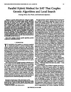
Inner approximation ( = 0:7; " = 0:4).
hence
Fig. 1.
and, finally
The idle-speed control problem consists in finding a control that maintains the engine speed within the desired range , with the following constraints on control inputs:
Therefore
which proves that , , , , is an –approximation of , , and . Since sequence (7) is controlled invariant with respect to there exists such that under Assumption 1 is such that is an –approximation of , we can conclude that
C. Application to Automotive Engine Idle-Speed Regulation The idle-speed control problem deals with the task of maintaining, while in the idle mode, the engine speed within a given range, rejecting torque disturbances generated by auxiliary subsystems such as the air-conditioning system and the steering wheel servo-mechanism, preventing the engine from turning off. The powertrain model we consider here is the following: (11) where is the engine speed expressed in revolutions per is the manifold pressure expressed in minute (RPM); mbar; is the momentum of inertia for , , , , are constants the transmission chain; , , ( , ); is the torque produced by the engine, given , the spark advance angle the efficiency function and the constant ; is the torque disturbance from acces). The two control inputs are the sory loads ( throttle opening angle and the spark advance angle .
We first linearize the model (11) about the “equilibrium” point: , , , . The resulting continuous-time linear system is then sampled using a zero order holder interpolator for the inputs. The problem we address consists in finding an –approximation of the maximal controlled invariant set contained in the set of state constraints, with respect to the discretized system denoted , with the input bounded by the input constraints. We therefore apply Algorithm 43 to the resulting system to find an -approximation of the maximal controlled invariant set that is itself controlled invariant. While the maximum disturbance allowed is 12 Nm, we asto reduce the number of iterations needed sume that but for the algorithm to converge. Thus, we expect that in the following we assume that this information is not available. Hence, we proceed as follows. 1) We set a desired value for the parameter , that determines how good the internal approximation should be. . Let 2) We then choose an initial value for , and, after having computed the corresponding inner approximation using Algorithm 43, we check whether it is an -approximation . If this of the maximal controlled invariant set, with is not the case, we repeat the procedure using a smaller , until we find the desired approximation. 3) At the same time, at each iteration we also compute the corresponding outer approximations, so as to have a lower and upper bound for the maximal controlled invariant set. . After six iterations, we obWe start by choosing tain the corresponding inner controlled invariant approximation shown in Fig. 1. The outer approximation found after six iterations is shown in the same figure. . Since The corresponding value of is the set does not satisfy our bound, we repeat the procedure, this
194
Fig. 2.
IEEE TRANSACTIONS ON AUTOMATIC CONTROL, VOL. 49, NO. 2, FEBRUARY 2004
Inner approximation ( = 0:95; " = 0:06).
time by choosing . After six iterations, we obtain the inner controlled invariant approximation shown in Fig. 2. The outer approximation found after six iterations is shown in the same figure. and the set is inThe value of is: deed an inner approximation of the maximal controlled invariant set with the required precision. V. CONCLUSION We presented a procedure for the determination of the maximal safe set for switching systems, which exploits the underlying structure of the discrete transitions. This procedure still suffers from the computational complexity stemming from the computation of maximal controlled invariant sets of general dynamical systems. This computation can be made more appealing if it is applied to a discretized version of the system. By doing so, well-known procedures for the computation of maximal controlled invariant sets for discrete-time linear systems can be used. Even for this simplified case, the procedure for the determination of the maximal controlled invariant set may not converge in a finite number of steps. For this reason, we presented an inner approximation procedure that, together with the classical outer approximation procedure, yields tight bounds for the error due to the truncation of the procedure after a finite number of steps. The features of our approach were presented by applying it to the idle speed regulation problem in the automotive engine control domain. REFERENCES [1] R. Alur, C. Courcoubetis, T. A. Henzinger, and P.-H. Ho, “Hybrid automata: An algorithmic approach to the specification and verification of hybrid systems,” in Hybrid Systems, R. L. Grossman, A. Nerode, A. P. Ravn, and H. Rischel, Eds. New York: Springer-Verlag, 1993, Lecture Notes in Computer Science, pp. 366–393. [2] J. P. Aubin, Viability Theory. Boston, MA: Birkhauser, 1991. [3] A. Balluchi, M. D. Di Benedetto, C. Pinello, C. Rossi, and A. Sangiovanni-Vincentelli, “Hybrid control in automotive applications: The cut-off control,” Automatica, vol. 35, 1999. [4] G. Basile and G. Marro, “On the robust controlled invariant,” Syst. Control Lett., no. 9, pp. 191–195, 1987.
[5] A. Bemporad, G. Ferrari-Trecate, and M. Morari, “Observability and controllability of piecewise affine and hybrid systems,” IEEE Trans. Automat. Contr., vol. 45, pp. 1864–1876, Oct. 2000. [6] L. Berardi, E. De Santis, and M. D. Di Benedetto, “Hybrid systems with safety specifications: Procedures for the computation and approximations of controlled invariant sets,” Univ. L’Aquila, Dept. Elect. Eng., Res. Rep. no. R.03–66, 2003. , “A structural approach to the control of switching systems with [7] an application to engine control,” presented at the 38th IEEE Conf. Decision Control, Phoenix, AZ, Dec. 7–10, 1999. [8] L. Berardi, E. De Santis, M. D. Di Benedetto, and G. Pola, “Controlled safe sets for continuous time linear systems,” in Proc. Eur. Control Conf. 2001, Porto, Sept. 4–7, 2001, pp. 803–808. [9] D. P. Bertsekas and I. B. Rhodes, “On the minimax reachability of target sets and target tubes,” Automatica, vol. 7, pp. 233–247, 1971. [10] F. Blanchini, “Constrained control for systems with unknown disturbances,” in Control and Dynamic Systems, C. T. Leondes, Ed. New York: Academic, 1992, vol. 51. , “Ultimate boundedness control for uncertain discrete-time sys[11] tems via set-induced Lyapunov functions,” IEEE Trans. Automat. Contr., vol. 39, pp. 428–433, Mar. 1994. [12] , “Set invariance in control—A survey,” Automatica, vol. 35, no. 11, pp. 1747–1768, Nov. 1999. [13] M. Broucke, “A geometric approach to bisimulation and verification of hybrid systems,” in Proc. HSCC’99, Hybrid Systems: Computation Control, vol. 1569, Lecture Notes in Computer Science, F. Vaandrager and J. H. van Schuppen, Eds., 1999, pp. 61–75. [14] P. Caravani and E. De Santis, “Doubly invariant equilibria of linear discrete time games,” Automatica, vol. 38, pp. 1531–1538, 2002. [15] A. Chutinan and B. H. Krogh, “Verification of polyhedral-invariant hybrid automata using polygonal flow pipe approximations,” in Proc. HSCC’99, Hybrid Systems: Computation and Control, vol. 1569, Lecture Notes in Computer Science, F. Vaandrager and J. H. van Schuppen, Eds., 1999, pp. 76–90. [16] P. d’Alessandro and E. De Santis, “Controlled invariance and feedback laws,” IEEE Trans. Automat. Contr., vol. 46, pp. 1141–1146, July 2001. [17] T. Dang, “Vérification et synthèse des systèmes hybrides,” Ph.D. dissertation, Institut National Polytechnique de Grenoble (Verimag), Grenoble, France, 2000. [18] T. Dang and O. Maler, “Reachability analysis via face lifting,” in Proc. 1st Int. Workshop, HSCC’98, Hybrid Systems: Computation Control, vol. 1386, Lecture Notes in Computer Science, S. Sastry and T. Henzinger, Eds., 1998, pp. 96–109. [19] E. De Santis, “On maximal invariant sets for discrete time linear systems with disturbances,” presented at the 3rd IEEE Med. Symp., Cyprus, Greece, 1995. [20] C. E. T. Dorea and J. C. Hennet, “Computation of maximal admissible sets of constrained linear systems,” in Proc. 4th IEEE Med. Symp., Krete, Greece, 1996, pp. 286–291. , “(A; B)-Invariance conditions of polyhedral domains for contin[21] uous-time systems,” Eur. J. Control, vol. 5, pp. 70–81, 1999. [22] L. Farina and L. Benvenuti, “Invariant polytopes of linear systems,” IMA J. Math. Control, Inform., vol. 15, pp. 233–240, 1998. [23] M. Greenstreet and I. Mitchell, “Reachability analysis using polygonal projections,” in HSCC’99, Hybrid Systems: Computation Control, vol. 1569, Lecture Notes in Computer Science, F. Vaandrager and J. H. van Schuppen, Eds., 1999, pp. 103–116. [24] P. O. Gutman and M. Cwikel, “Admissible sets and feedback control for discrete-time linear dynamical systems with bounded controls and states,” IEEE Trans. Automat. Contr., vol. AC-31, pp. 373–376, Mar. 1986. [25] S. S. Keerthi and E. G. Gilbert, “Computation of minimum-time feedback control laws for discrete-time systems with state-control constraints,” IEEE Trans. Automat. Contr., vol. AC-32, pp. 432–435, Mar. 1987. [26] J. L. Kelley and I. Namioka, Linear Topological Spaces. New York: Springer-Verlag, 1963. [27] A. B. Kurzhanski and P. Varaiya, “Ellipsoidal techniques for reachability analysis,” in Proc. 3rd Int. Workshop, HSCC’00, Hybrid Systems: Computation Control, vol. 1790, Lecture Notes in Computer Science, N. Lynch and B. H. Krogh, Eds., 2000, pp. 202–214. [28] J. Lygeros, C. Tomlin, and S. Sastry, “Controllers for reachability specifications for hybrid systems,” Automatica, vol. 35, 1999. [29] I. Mitchell and C. Tomlin, “Level set methods for computation in hybrid systems,” in Proc. 3rd Int. Workshop, HSCC’00, Hybrid Systems: Computation Control, vol. 1790, Lecture Notes in Computer Science, N. Lynch and B. H. Krogh, Eds., 2000, pp. 310–323.
DE SANTIS et al.: COMPUTATION OF MAXIMAL SAFE SETS FOR SWITCHING SYSTEMS
[30]
[31] [32]
[33] [34]
[35]
[36]
, “Validating a Hamilton–Jacobi approximation to reachable sets,” in Proc. 4th Int. Workshop, HSCC’01, Hybrid Systems: Computation Control, vol. 2034, Lecture Notes in Computer Science, M. D. Di Benedetto and A. Sangiovanni-Vincentelli, Eds., 2001, pp. 418–432. A. S. Morse, “Supervisory control of families of linear set-point controllers—Part 1: Exact matching,” IEEE Trans. Automat. Contr., vol. 41, pp. 1413–1431, Oct. 1996. O. Shakernia, G. P. Pappas, and S. Sastry, “Decidable controller synthesis for classes of linear systems,” in Proc. 3rd Int. Workshop, HSCC’00, Hybrid Systems: Computation Control, vol. 1790, Lecture Notes in Computer Science, N. Lynch and B. H. Krogh, Eds., 2000, pp. 407–420. J. S. Shamma, “Optimization of the l -induced norm under full state feedback,” IEEE Trans. Automat. Contr., vol. 41, pp. 533–544, Apr. 1996. C. Tomlin, J. Lygeros, and S. Sastry, “Synthesizing controllers for nonlinear hybrid systems,” in Proc. 1st Int. Workshop, HSCC’98, Hybrid Systems: Computation Control, vol. 1386, Lecture Notes in Computer Science, S. Sastry and T. Henzinger, Eds., 1998, pp. 360–373. , “Computing controllers for nonlinear hybrid systems,” in Proc. HSCC’99, Hybrid Systems: Computation Control, vol. 1569, Lecture Notes in Computer Science, F. Vaandrager and J. H. van Schuppen, Eds., 1999, pp. 238–255. R. Vidal, S. Schaffert, J. Lygeros, and S. Sastry, “Controlled invariance of discrete time systems,” in Proc. 3rd Int. Workshop, HSCC’00, Hybrid Systems: Computation Control, vol. 1790, Lecture Notes in Computer Science, N. Lynch and B. H. Krogh, Eds., 2000, pp. 437–450.
Elena De Santis (M’04) graduated in electrical engineering (summa cum laude) at the University of L’Aquila, L’Aquila, Italy, in 1983. From 1987 to 1998, she had been a Researcher, and since 1998, an Associate Professor of Automatic Control at the same university. She has published papers in the fields of analysis, control and optimization of constrained dynamical systems, dynamic model management in decision support systems (DSS), analysis and control of uncertain systems, positive systems, and dynamic games. Her current research interests lie in the fields of constrained dynamical systems and hybrid systems.
195
Maria Domenica Di Benedetto (F’00) received the Dr. Ing. degree (summa cum laude) in electrical engineering and computer science from the University of Rome “La Sapienza,” Rome, Italy, in 1976 and the “Docteur-Ingénieur”and “Doctorat d’Etat ès Sciences” degrees from the Université de Paris-Sud, Orsay, France, in 1981 and 1987, respectively. From 1979 to 1983, she was a Research Engineer at the scientific centers of IBM in Paris and Rome. From 1983 to 1987, she was an Assistant Professor at the University of Rome “La Sapienza.” From 1987 to 1990, she had been Associate Professor at the Istituto Universitario Navale of Naples, Italy. From 1990 to 1993, she was Associate Professor at the University of Rome “La Sapienza”. Since 1994, she has been Professor of Control Theory at University of L’Aquila. From 1995 to 2002, she was Adjunct Professor, Department of EECS, University of California at Berkeley. In 1987, she was Visiting Scientist at the Massachusette Iinstitute of Technology, Cambridge; in 1988, 1989, and 1992, she was a Visiting Professor at the University of Michigan, Ann Arbor; in 1992, Chercheur Associé, C.N.R.S., Poste Rouge, Ecole Nationale Supérieure de Mécanique, Nantes, France; in 1990, 1992, 1994 and 1995, McKay Professor at the University of California at Berkeley. Her research interests revolve around nonlinear control and hybrid systems. Since 2000, she has been Director of the Center of Excellence for Research DEWS on “Architectures and Design methodologies for Embedded controllers, Wireless interconnect and System-on-chip,” University of L’Aquila. Dr. Di Benedetto was Associate Editor of the IEEE TRANSACTIONS ON AUTOMATIC CONTROL and has been Subject Editor of the International Journal of Robust and Nonlinear Control. She is a Chairperson of the Standing Committee on Fellow Nominations, IEEE Control Systems Society.
Luca Berardi graduated in electrical engineering (summa cum laude) at the University of L’Aquila, L’Aquila, Italy, in 1996, and received the Ph.D. degree in systems engineering from the University of Rome “La Sapienza,” in 2001. In 1997, he worked at CSELT, the research center of Telecom Italia, Turin, Italy. Since 2001, he has been a Postdoctoral Fellow with the Electrical Engineering Department at the University of L’Aquila. His current research interests are control of hybrid systems and application of stochastic and robust control methodologies to mathematical finance.