calculator and does not compute confidence intervals. .... ON FIRST CALL DNEW HAS USER INITIAL VALUE IF IOPT=0. * U = .... Center, University of Maryland.
APPLIED AND ENVIRONMENTAL MICROBIOLOGY, May 1983, p. 1646-1650
Vol. 45, No. 5
0099-2240/83/051646-05$02.00/0
Copyright © 1983, American Society for Microbiology
Computation of Most Probable Numbers ESTELLE RUSSEK1 AND RITA R. COLWELL2*
Department of Animal Sciences' and Department of Microbiology,2 University of Maryland, College Park, Maryland 20742
Received 21 September 1982/Accepted 29 December 1982
A rapid computational method for maximum likelihood estimation of mostprobable-number values, incorporating a modified Newton-Raphson method, is presented. The method offers a much greater reliability for the most-probablenumber estimate of total viable bacteria, i.e., those capable of growth in laboratory media. The most-probable-number (MPN) method is an important technique for microbiologists in the enumeration of viable bacteria in samples of food, water, and natural products. The method has undergone some evolution (3), but the principle itself is essentially unchanged since it was first developed. Some samples do not lend themselves to viable bacterial enumeration by any other procedures, so the MPN technique is convenient and necessary in some instances, and its use will continue. Many uses for MPN have been described in the literature in the fields of food microbiology, water quality, and public health (3, 9). MPN methods have been treated statistically by a number of investigators (deMan [5, 6], Finney [7], Halvorson and Ziegler [8], Moran [12], and Taylor [15]), but the general computation has not changed significantly. We report here a rapid computational method for maximum likelihood estimation of MPN values utilized in existing tables (1), incorporating a modified Newton-Raphson method, as discussed by Kalbfleisch and Prentice (10). Use of such an algorithm eliminates the need for tables, but also, more importantly, allows an investigator to select the number of dilutions and replicates per dilution according to individual need. The method presented produces d (the MPN), its standard error, and a 95% confidence interval. In contrast to the method discussed by deMan (5), it does not eliminate improbable values; deMan's method can yield confidence intervals that are not truly 95% intervals. Obtaining unlikely extremes is more often the product of bacteria not being randomly dispersed throughout the medium. Such values invalidate the use of MPN tables, but can be detected by using a test proposed by Moran (12) or, if the number of replicates per dilution is large, by using the method described here. Finney (7) discusses a method for fitting MPN, based on weighted least squares. With
large numbers of replicates per dilution, results should be equivalent to those based on maximum likelihood. However, as pointed out by Finney (7), this approach presents problems if the bacterial concentrations are low and the proportion of positives is small. Maximum likelihood estimates offer some advantages in this regard, but both approaches allow computation of confidence intervals. Winter (16) suggests an alternative method for computing MPN values; this method, however, corresponds to neither of the above. The MPN resulting from the computations presented here corresponds to that presented by Koch (11) and Cochran (2). However, Koch (11) presents an algorithm which is dependent upon an HP41C calculator and does not compute confidence intervals. Cochran's method for formulating confidence limits involves the use of a table, whereas the method presented here does not. Most of the methods used in the computation of interval estimates for MPN values are based on a large number of replicates. While the term "large" is vague, what it means is that the larger the number of replicates per dilution, the more robust the 95% confidence interval. Since it is not economically feasible, or even practical, in many cases to run hundreds of replicates per MPN, a simple simulation study is provided as an example of the ability to study small-sample properties where the methods are employed. This simulation study is preferable because with a simulation one is assured that the assumptions of the model are correct. Methods which cannot perform adequately when assumptions hold cannot be expected to perform at all when assumptions fail. In addition, since the true concentration is known, i.e., fixed in advance, problems of validation are minimized. MATERIALS AND METHODS Statistical model. Assuming there are k dilution levels (k .-1) with: v, = volume in ith dilution (i = 1,
1646
COMPUTATION OF MOST PROBABLE NUMBERS
VOL. 45, 1983
. . ., k); ni = number of replicates in ith dilution; and si = number of sterile tubes in ith dilution. The assumption of bacteria randomly dispersed leads to the probability of observing si sterile tubes being:
P(s1) = (ni) (e-v)(i
-
vn-
j
(1)
Since the outcomes at each dilution are statistically independent, solving for d involves finding the d that maximizes P(sj) x F(s2) x ... x P(sk). This leads to finding the d that solves: k
i=1
k
visi =
is-1
(ni - s,)/(evid
-
1)
(2)
Computational method. The computational method used is described by Kalbfleisch and Prentice (10) and utilizes maximum-likelihood methods. First, an initial estimate for d is made. The computer can do this by using data for those dilution levels where the percentage of sterile samples, i.e., no growth, lies between 0 and 100, i.e., excluding all negative or all positive dilutions. Then, one can use the average of -(1/v,) log (s/n1) for these concentrations. Alternatively, a reasonable guess can be specified by the user. As long as this guess is within an order of magnitude, and strictly greater than zero, the method works. Once an initial guess is specified, one computes:
dNEW
=
dOLD
+
U(dOLD)/I(doLD)
where: k
U(dOLD)
k
nivA/(e OLD 1) iS=1
= E
Vs,
i= 1
and: k
(dOLD)
=
E
niv.2/(evIOLD 1) -
where doLD is the initial guess during the first iteration. The value of dNEW is then called doLD, and the procedure is repeated until little or no change in the value of d occurs. If the initial guess is a good one, very few iterations are needed. One of the attractive features of the algorithm is that it provides the 95% confidence interval for d as described by Cochran (2) and Parnow (13), i.e., by noting that the standard error for d is approximately 1/VId and the standard error for ln(d) (In denotes the logarithm, base e, e = 2.71 ... ) is approximated by 1/[dVI-j]. When the number of replicates is large, a 95% confidence interval for d is d + 1.96 SE(d). However, as indicated by Cochran (2) and Finney (7), using ln(d) + 1.96 SE[ln(d)] and taking anti-logs is a better approach. Goodness-of-fit tests. As indicated earlier, the derivation of MPN assumes that bacteria are randomly dispersed throughout the sample. Obvious violations
1647
exist when replicates for more diluted media yield more positive values than the original, a result that may be caused by clumping, affinity of the bacteria for the surface or walls of the test tube, or heterogeneity in the medium itself. Not rejecting a null hypothesis of randomness does not guarantee randomness, but rather is a rejection of situations in which randomness appears to be markedly violated. With very high bacterial concentrations, randomness becomes more difficult to achieve, because the MPN model assumes bacteria occupy an infinitesimal proportion of the space available, and achieving adequate mixing is difficult. With 10-fold dilutions, violations may be obvious. With twofold dilutions they may be less so. Moran (12) suggests a test which rejects randomness if T = lsi(n - s,) is large. This test is quite easy to perform with 2fold dilutions, but less so in 5- and 10-fold series, because of computations associated with the standard error of T. However, when k 2 2 a simple x2 test can be derived by using the maximum likelihood estimate derived above. Let Ei = n,ie`. Then:
X2= i=E (S-Ei)2 (Si] Ei ni - Ei (-
k
ni(si - E,)2EXni - E) If x2 is greater than x2 table value with k - 1 degrees of freedom (e.g., k = 2, use value 3.841; k = 3, use value 5.991), randomness is rejected. However, as is true of most x2 goodness-of-fit tests, it is advisable that Ei and ni - Ei should be large (some suggest greater than 5). Although the number of replicates required is large, this test for randomness need not be done with every MPN performed, but only at the initial stages and perhaps repeated later on to assure validity of the method. This test is a straightforward application of methods described by Rao (14). Simulation. A technique commonly used to test the validity of statistical methods based on large sample approximations, as in the case of standard errors and confidence intervals presented here, is that of a Monte Carlo simulation. One can, in effect, simulate hundreds of replicate samples from the same "population." In this study, 500 samples were generated (using the IMSL routine GGBIR) from each population defined, using values of ni, vi, and d commonly found in practice. Values of d were chosen according to the suggestion of Cochran (2), i.e., that one chooses volumes so that d falls between 1 and 2 (the volume of the original undiluted replicates being 1). Tests and estimates which do not meet such expectations, in fact, should not be employed in a laboratory. For each sample generated, the MPN and its confidence interval were recorded, and the results were tallied. An illustration of the computational method is presented in Fig. 1. With 500 replicates, approximately 95% or 475 confidence intervals should contain d. To demonstrate the usefulness, or lack thereof, of confidence intervals, the average length of the confidence interval was recorded for each population. Confidence intervals which are wide are not very informative, but indicate that the value obtained for
APPL. ENVIRON. MICROBIOL.
RUSSEK AND COLWELL
1648
REAL N (10) ,S (10) ,V(10) kPROGRAM TO COMPUTE MPN FOR NDIL DILUTIONS(LE 10), k ARBITRARY NO PER DILUTION, N-FOLD DILUTIONS k N IS THE ARRAY HOLDING NO OF REPS PER DILUTION k S IS THE NUMBER OF STERILE TUBES PER DILUTION k V IS THE VOLUME OF ORIGINAL LIQUID IN DILUTION 5 READ (5,6,END=3200) NDIL,NFOLD,IOPT 6 FORMAT (I2,I3,I1) IF (NDIL .GT. 10) STOP READ (5,20) CONV,DNEW, (N(I),I=1,NDIL),(S(I),I=1,NDIL) 20 FORMAT (2F10.4,10F5.0/1OF5.0)
WRITE (6,25) CONV,NFOLD,IOPT
25 FORMAT ( ' CONVERGENCE,CRITERIA=',F1O.4,2X,I5, '-FOLD DILUTION' 1 , ' OPTION CODE=',1l DO 40 I=1,NDIL 40 V(I) =1./NFOLD** (I-1) CALL MLE(N,V,S,NDIL,DNEW,IOPT,CONV) GO TO 5 3200 STOP END SUBROUTINE MLE(N,V,S,NDIL,DNEW,IOPT,CONV) REAL N(NDIL) ,V(NDIL) ,S (NDIL) * ON FIRST CALL DNEW HAS USER INITIAL VALUE IF IOPT=0 * U = ESTIMATED SCORE FUNCTION * FISHER = INFORMATION VALUE *IOPT=0 USE LEAST SQUARE EST, IOPT-0 USE USER GIVEN VALUE *CONV=HOW CLOSE DOLD AND DNEW NEED TO BE TO STOP ITERATION(E.G. CONVz.001) *N(I)=NUMBER OF TUBES IN ITH DILUTION *V(I)= VOLUME OF ORIGINAL SAMPLE IN ITH DILUTION *E.G. DILUTION I 1 2 3 *
-
* *
N(I) 5 V(I) 1.0 IF (IOPT .EQ. 0) THEN DOLD = DNEW ELSE DOLD = 0. JJ = 0 DO 10 I=1,NDIL
-
-
-
-
-
-
-
-
-
-
-
-
-
5
5 .5
.25
-
5 PER DIL 2-FOLD
.OR. .LT. .1) IF((ABS(N(I)-S(I)) (S5(I) .LT. .1) ) GO TO 10 DOLD = DOLD + ALOG(N(I)/S (I) )/V(I) JJ = JJ + 1 CONTINUE IF(JJ .EQ. 0) THEN DOLD = AMAXO (DNEW, 1. 5) ELSE DOLD = DOLD/JJ ENDIF ENDIF
1
10
DO 100 I=1,100 * UP TO 100 ROUNDS OF ITERATION FOR THE LIKELIHOOD ESTIMATE U=O. FISHER=0. * ALGORITHM IS MODIFIED NEWTON-RAPHSON AS DESCRIBED IN * KALBFLEISH AND PRENTICE SURVIVAL ANALYSIS TEXT DO 50 J=1,NDIL
EVD=EXP(V(J)*DOLD)-1. U=U-S (J) *V(J) +N (J) -S (J) ) *V (J)/EV
50
FISHER=FISHER+N(J)*V(J)**2/EVD DNEW=DOLD+U/F IS HER
IF (ABS(DNEW-DOLD) .LT. CONV) GO TO 200 100 DOLD = DNEW *WHEN SIMULATION WAS DONE--NO FAILURES WERE NOTED WRITE (6,120) DNEW 120 FORMAT (' FAILURE TO CONVERGE' ,F10.5) RETURN C COMPUTE CONF. INTERVAL AROUND LN(D),I(D)=FISHER INFO 200 SE=EXP (1.96/ (SQRT (FISHER) *DNEW))
210
CLLOW=DNEW/S E CLHIGH=DNEW*SE WRITE(6,210) DNEW,CLLOW,CLHIGH FORMAT(' MPN=',F1O.5,' 95% CONF.LIMITS (',F1O.5,',',F1O.S,')') RETURN END
FIG. 1. Fortran program illustrating MPN algorithm.
VOL. 45, 1983
COMPUTATION OF MOST PROBABLE NUMBERS
TABLE 1. Number of times the true value of MPN was included in the 95% confidence interval (k = 3, nf = n2 = n3 = n)a 2-fold dilution n =5 n = 10
d
10-fold dilution n=5
n = 10
1.00 482 469 467 476 1.25 466 472 489 463 1.50 469 478 473 464 1.75 478 467 482 471 2.00 478 479 473 474 3.00 480 476 486 477 a Each set of parameters was replicated 500 times.
the MPN is highly variable and that if one repeated the test with another sample from the same volume the results might not be duplicated. Using MPN values, with large standard errors, in subsequent analyses may obscure relationships with other factors when the MPN values are themselves very imprecise.
RESULTS AND DISCUSSION A total of 9,000 MPN dilution series were generated and evaluated in less than 38 s on a Univac 1100/82. The results of the simulation are
1649
presented in Tables 1 and 2. In spite of the fact that confidence intervals for MPN values are based on large-sample theory, the intervals one obtains do contain the true MPN value about 95% of the time, i.e., about 475 of 500 cases. This result indicates the use of log MPN in subsequent analyses such as an analysis of variance. If the MPN values vary considerably, a weighted analysis of variance (weights inversely proportional to their variance) may be better employed. However, it should be noted that the MPN method does slightly overestimate the bacterial concentrations present. Using 10-fold rather than 2-fold (i.e., serological) dilutions yields higher standard errors, as might be expected. Using a larger number of replicates per dilution obviously will reduce variability as well as bias. The use of either 5 or 10 replicates per dilution yields an average confidence interval of about 1.2 to 2.3 on a natural log scale, or about 0.52 to 1.00 on a log base 10 scale, suggesting that one can estimate densities within an order of magnitude. However, less than five replicates per dilution is inadequate. In addition, an average confidence interval length of 1.00 on a log10 scale suggests that many of the intervals were in
TABLE 2. Sample statistics provided for the example given in the text No. of
replications
Dilution
Tu
Trdue
Confidence SapeTuSapevg interval avg Savgple (In MPN) lTn(d) MPNlegh
S
2-fold
1.00 1.25 1.50 1.75 2.00 3.00
1.0597 1.3319 1.5959 1.8684 2.2252 3.2539
0 0.2231 0.4055
10-fold
1.00 1.25 1.50 1.75 2.00 3.00
2-fold
1.00 1.25 1.50 1.75 2.00 3.00
per dilution
10
1.0986
-0.0333 0.1914 0.3874 0.5447 0.7289 1.1188
1.6728 1.5729 1.4973 1.4574 1.4227 1.4157
1.2445 1.4629 1.8676 2.1228 2.5747 3.7970
0 0.2231 0.4055 0.5596 0.6931 1.0986
0.0211 0.2072 0.5888 0.5902 0.7911 1.2010
2.2524 2.1478 2.0709 2.0452 2.0469 2.0779
1.0636 1.3041 1.5541 1.8171 2.1021 3.1531
0 0.2231 0.4055
0.0131 0.2252 0.4066 0.5587 0.7108 1.1174
1.1499 1.0827 1.0382 1.0129 0.9925 0.9880
0.55% 0.6931
0.5596 0.6931 1.0986
-0.0005 0 1.0882 1.5385 1.00 0.2231 0.2600 1.25 1.4052 1.4568 0.4055 0.4460 1.6933 1.4251 1.50 0.55% 0.5827 1.9257 1.75 1.4060 0.6931 0.7389 2.2502 1.4059 2.00 3.00 3.3947 1.0986 1.1497 1.4569 a 0.43429. Each to To convert are taken. before Average length on natural-log scale, anti-logs log1o multiply by line represents the average of 500 samples.
10-fold
1650
RUSSEK AND COLWELL
fact larger than 1.0 in width. For comparing two sites or treatments, typically one will need to analyze more MPN values per treatment or site than direct counts, because of the larger standard error associated with the MPN values. If one is collecting environmental data, where changes of less than an order of magnitude in bacterial counts may be microbiologically significant, MPN values would probably not be a reasonable approach, unless the investigator is willing to increase greatly the number of replicates per dilution and the number of dilution concentrations. Finally, the results of the simulation presented here suggest some strategies that can be developed for choosing sample sizes. Using the same number of replicates per dilution is a simple procedure but, under most circumstances, not optimal. If one selects three dilutl*ons, as is often the case at present, with the intention that the highest concentration will yield almost all positive reactions and the lowest concentration will yield uniformly negative reactions, it is logical to replicate the middle concentration more than the upper and lower. After all, whenever the result is all or nothing, the variability observed is quite small. It is only when the results vary over a wide range, e.g., any value between 0 and 100%, that larger samples are required. This approach can be followed after a number of similar samples have been analyzed to assure that the assumptions made regarding the highest and lowest concentrations are, in fact, valid. MPN values will continue to be used in microbiology, because alternative methods for estimating bacterial numbers have not yet been developed for those conditions where direct viable counts by epifluorescent microscopy (4) are too tedious or a problem because of large amounts of particulate matter present in the sample, or where a rapid estimate of viable bacteria, i.e., those bacteria capable of growth on selective media, is needed. The approach offered here provides a much greater reliability for the MPN estimate.
APPL. ENVIRON. MICROBIOL. ACKNOWLEDGMENTS This work is a result of research sponsored (in part) by World Health Organization grant C6/181/70 and by National Oceanic and Atmospheric Administration Office of Sea Grant, Department of Commerce, under grant no. NA81AA-D-00040. Computer time was made available by Computer Science Center, University of Maryland. LITERATURE CITED 1. American Public Health Association. 1971. Standard methods for the examination of water and waste water, p. 635678. American Public Health Association, Washington, D.C. 2. Cochran, W. G. 1950. Estimation of bacterial densities by means of the "most probable number." Biometrics 5:105116. 3. Colwell, R. R. 1979. Enumeration of specific populations by the Most-Probable-Number (MPN) method, p. 56-61. In J. W. Costerton and R. R. Colwell (ed.), Native aquatic bacteria: enumeration, activity and ecology, ASTM STP. 695. American Society for Testing and Materials, Philadelphia, Pa. 4. Daley, R. J., and J. E. Hobble. 1975. Direct counts of aquatic bacteria by a modified epifluorescence technique. Limnol. Oceanogr. 20:875-882. 5. deMan, J. C. 1975. The probability of most probable numbers. Eur. J. Appl. Microbiol. 1:67-78. 6. deMan, J. C. 1977. MPN tables for more than one test. Eur. J. Appl. Microbiol. 4:307-316. 7. Finney, D. J. 1978. Statistical method in biological assay, 3rd ed. Macmillan Publishing Co., New York. 8. Halvorson, H. O., and N. R. Ziegler. 1933. Application of statistics to problems in bacteriology. III. A consideration of the accuracy of dilution data obtained by using several dilutions. J. Bacteriol. 26:559-567. 9. Hoskins, J. K. 1933. The most probable numbers of B. coli in water analysis. J. Am. Water Works Assoc. 25:867877. 10. Kalbfleisch, J. D., and R. L. Prentice. 1980. The statistical analysis of failure time data. Wiley and Sons, New York. 11. Koch, A. L. 1982. Estimation of the most probable number with a programmable pocket calculator. Appl. Environ. Microbiol. 43:488-490. 12. Moran, P. A. P. 1954. The dilution assay of viruses. J. Hyg. 52:189-193. 13. Parnow, R. J. 1972. Computer program estimates of bacterial densities by means of the most probable numbers. J. Food Technol. 7:56-62. 14. Rao, C. R. 1973. Linear statistical inference, 2nd ed. John Wiley & Sons, New York. 15. Taylor, J. 1962. The estimation of numbers of bacteria by ten-fold dilution series. J. Appl. Bacteriol. 25:54-61. 16. Winter, J. 1978. Microbiological methods for monitoring the environment, p. 78-86. Water and Wastes. EPA600/8-78-017. Environmental Protection Agency, Washington, D.C.