... being the constant speed in. American Institute of Aeronautics and Astronautics ..... Transactions of Royal Society of London A255, 469-. 503. [13] GOLDSTEIN ...
Copyright ©1996, American Institute of Aeronautics and Astronautics, Inc. AIAA Meeting Papers on Disc, May 1996 A9630845, AIAA Paper 96-1732
Computation of noise generation and propagation for free and confined turbulent flows C. Bailly Electricite de France, Clamart
P. Lafon Electricite de France, Clamart
S. Candel Paris, Ecole Centrale, Chatenay-Malabry, France
AIAA and CEAS, Aeroacoustics Conference, 2nd, State College, PA, May 6-8, 1996 This paper deals with the application of the SNGR (Stochastic Noise Generation and Radiation) model to compute turbulent mixing noise generated in a duct obstructed by a diaphragm. Two problems must be solved in the framework of an acoustic analogy. First, a wave operator must be derived for sound waves traveling in any mean flow. In the SNGR model, the system of linearized Euler equations is used. An expression of the source term is then deduced from the conservation laws of motion and can be simplified with classical assumptions of aeroacoustics in the case of subsonic mixing noise. Secondly, the knowledge of the turbulence velocity field is required to compute this source term. In the SNGR model, the space-time turbulence velocity field is generated by a sum of random Fourier modes. Finally, the radiated acoustic field is calculated numerically by solving the inhomogeneous propagation system. The method is applied to the case of a 2D duct obstructed by a diaphragm. Numerical results are compared with available experimental ones. Computed noise levels closely match experimental ones and follow the expected U4 law. (Author)
Page 1
96-1732
A96-30845
Computation of noise generation and propagation for free and confined turbulent flows C. Bailly*, P. Lafon* Departement Acoustique et Mecanique Vibratoire Electricite de France, Direction des Etudes et Recherches 1 av. du General de Gaulle, 92141 Clamart Cedex, Prance S. Candel*
Laboratoire EM2C, Ecole Centrale Paris 92295 Chatenay-Malabry Cedex, France
Abstract
tion and its source term. It is also necessary to provide some informations about the turbulence in the flow. Classical aeroacoustic approaches based on the Lighthill acoustic analogy generally use the free-space Green's function in order to solve the wave equation, but the application of such techniques to confined configurations are not straightforward. In this paper, we use the Stochastic Noise Generation and Radiation model (SNGR),2'4'6'19 which solves the system of linearized Euler equations instead of a wave equation and uses as input a synthesized turbulent field providing the source term. The equations of the SNGR model are presented in section 2. It is shown- in section 3 how one may synthesize a space-time turbulent velocity field with suitable statistical properties. The application to the case of a duct obstructed by a diaphragm is discussed in section 4.
This paper deals with, the application of the SNGR ( Stochastic Noise Generation and Radiation) model to compute turbulent mixing noise generated in a duct obstructed by a diaphragm. Two problems must be solved in the framework of an acoustic analogy. First, a wave operator must be derived for sound waves travelling in any mean flow. In the SNGR model, the system of linearized Euler equations is used. An expression of the source term is then deduced from the conservation laws of motion, and can be simplified with classical assumptions of aeroacoustics in the case of subsonic mixing noise. Secondly, the knowledge of the turbulence velocity field is required to compute this source term. In the SNGR model, the spacetime turbulence velocity field is generated by a sum of random Fourier modes. Finally, the radiated acoustic field is calculated numerically by solving the inhomogeneous propagation system. The method is applied in this paper Propagation in nonuniform mean flow to the case of a two-dimensional duct obstructed by a diaphragm. Numerical results are compared with available The simplest wave equation that one can exactly deexperimental ones. Computed noise levels closely match rive from the fundamental conservation laws of motion is experimental ones and follow the expected U* law. Lighthill's equation:20'21 Introduction (1)
Aeroacoustic calculations usually require a wave equa-
where p is the density and Ty is Lighthill's tensor Tij = pUiUj-\- (p — c2/>) _Sij — TIJ. In this last expression, ut p, and URA 263 CNRS, Eeoie Centrale de Lyon, 36 av. G. de Coliongue, T designate the velocity, pressure and viscous stress tensor. 69131 Ecully Cedex, Prance Here one assumes that the medium external to the flow is 'Research Scientist, Member AIAA ^Professor, Member AIAA homogeneous and at rest, c0 being the constant speed in * Assistant Professor, Member AIAA. Present address: LMFA,
Copyright ©1996 by the American Institute of Aeronautics and Astronautics, Inc. All rights reserved
American Institute of Aeronautics and Astronautics
this ambient medium. The free-space Green's function
This equation shows that Phillips' wave operator does of this wave operator is known allowing easy application not contain all the terms that appear in (5). On the other of Lighthill's analogy in many studies.1'3'7'12-14'25 The hand, in the case of a sheared mean flow, the simplest wave
method does not account for mean flow effects on acoustic wave propagation. Such effects are known to modify the aerodynamic noise spectrum and directivity. Phillips24 replaced Lighthill's equation by a convected wave equation where a part of the mean flow effects were included in the wave operator rather than in the source term. Introducing the logarithm of the pressure variable TT = Inp, Phillips' equation reads:
dt2
=
dxi
.v J
equation for the acoustic variable if1 is a third order differential equation. Lilley22 derived such a third order wave equation from Phillips' equation with this idea. Thus, in applying the convective D/Dt operator to Phillips' equation (3), it follows: _ dt \ dt* ~ 8x dui duj duk •=• —27—— •5-'- -5— + other terms
2
——
dxj .
-
dt Vc» dt
pdxj
where 7 = CP/CU is the specific heats ratio. One sees that the main source term for jet noise only contains components of the velocity field unlike Lighthill's source term. At high Reynolds numbers, the viscous stress tensor can be neglected. Furthermore, one assumes viscous dissipation and heat conduction effects are negligible in sound generation and propagation. Then assuming a parallel sheared
mean flow: u» = U (zj) 6ii +«i, Phillips' equation (3) may be written in the form: dU
where the viscous contribution and the entropy fluctuations are neglected. The free-space Green function of the Lilley's equation is unknown and it is difficult to solve numerically a third order wave equation, unlike the linearized Euler's equations. Moreover, in the case of a nonuniform mean flow, acoustic and hydrodynamic fluctuations can not be clearly separated to form a wave operator.8'23'28 Thus, computation of the acoustic field by solving linearized Euler's equations contitutes an interesting alternative. An analysis of the acoustic analogy associated with linearized Euler's equations was developed.2'6 It was found that the following system of two first-order equations has to be retained:
(3)
Dt*
^ ,... M,../^
=
0
+ 3
*
J
* )
where
du'j
dUj
dt
"^M
, duj0
1 dp?
&•£?*
Po &&i
D_ (7) where the source term reads as follows: ~Dt is the convective time derivation operator. It is also known that linearized Euler's equations govern acoustic wave j Jf propagation. So, the associated wave equation should be identical to the previous homogeneous equation. But this The subscript o designates a value of the mean flowfield is not exactly the case.10'22 Indeed, assuming a global and the subscript t a value of the turbulent field, u' and 2 isentropic relation dp = c dp, the wave equation derived pf are the acoustic velocity and pressure. The left hand from the linearized Euler's equation is given by: side of (7) is the system of the linearized Euler's equations around a stationary mean flow (U0,p0,p0). *s
2
Dt
~ £>•»•
I
\
2 ___*"
C
° fi-».
I
O
I ~
^*V
^ ""g
*f J~~ &•*-
_
/y|\
^
'
In order to eliminate the term containing velocity fluctuations of the wave operator, one must again apply the D/Dt operator to the last equation. This finally yields:
The right
hand side of this system is the acoustic source term, which is nonlinear in velocity fluctuations. However, the time average of the source term is zero. The previous system
(7) is derived under the following assumptions. Acoustic pressure fluctuations are isentropic, the turbulent veloc-
ity is incompressible, and only the first order interaction between the mean flow and the acoustic field is retained.
Dt
Dt*
dz2 (5)
In other words, phenomena such as scattering of sound by turbulence are assumed to be negligible.
American Institute of Aeronautics and Astronautics
Finally, to compute the sound field, one carries out the three following steps:
= 1v /° Jo where k is the kinetic energy per mass unit and e the rate of dissipation, that is to say the rate of transfer of kinetic energy per mass unit and per time unit. These two local values of the turbulent field may be used to estimate the integral length scale L:
(i) An aerodynamic calculation of the mean flow is performed by solving the averaged Navier-Stokes equations with a k — e turbulence closure. (ii) A space-time stochastic turbulent velocity field is generated as a sum of random Fourier modes.
L=
(iii) The propagation system (7) is solved. In the left hand side, one uses values of the mean flowfield calculated in the first step as coefficients of the two first-order differential equations. On the
r°° / ( r ) d r ~
Jb3/2
Jo
A characteristic angular frequency for the turbulence is given for each mode by the relation:5'26
right hand side, the acoustic source term S is calculated from the synthetized turbulent field.
w, = e1/3*2/3
A space-time stochastic turbulent velocity field
(9)
Application to the case of a duct obstructed by a diaphragm
A method to simulate a spatial stochastic turbulent velocity field was initially devised by Kraichnan17 and Kar-
The SNGR model was first applied to cases of axisymweit.15 Their Fourier mode approach is used but a spacemetric subsonic jets.2'4'6 The configuration of the 2D duct time evolution of the turbulent field u is introduced by obtructed by a diaphragm (see figure 1) has already been writing that: studied27 and we here use the same aerodynamic results. |£ + Uc.Vu = 0
where Uc is the convection velocity. In what follows, the subscript t which designates the turbulent velocity field is omitted. The turbulent velocity field is given by the following sum of N modes: 60 cm
14.6 cm
JV U (x, t) = 2 ^ «„ COS [kn. (X - tU e ) + V-n + Unt] ffn n=l
(8)
where kn is the wave vector picked randomly on a sphere to ensure a statistical isotropy at time zero. As a consequence of the incompressibility of the turbulent velocity field, kn.o-n = 0 for each mode n. ij>n is chosen with uniform probability to obtain an homogeneous field. The amplitude u of each mode is determined from a modified Von Karman spectrum to simulate the complete spectral range:
Figure 1: Sketch of the geometry. Aerodynamic results The mean flowfield is calculated as a numerical solution of the average Navier-Stokes equations associated with a k — e turbulence closure. These calculations are carried
out with the ESTET code developed by the "Laboratoire National Hydraulique" of the "Direction des Etudes et Recherches d'Electricite de France" and are performed on tin = a grid of 190 x 83 points. The mesh is finer close to the diaphragm. The smallest mesh size is 1.0 x 10~3 m and exp 17/6 the largest is 5.0 x 10~3 m. The computational domain (k/k e ) 2 ] is displayed in figure 2 and a view of the grid close to the diaphragm is shown in figure 3. It is not necessary where k,, = e1/4!/3/4 is the Kolmogorov wave number. The to discretize a large part of the duct upstream of the diparameters a and ke of the spectrum are determined from aphragm. The two main parameters for these calculations the-two integral relations which defined and e: are the aperture e of the diaphragm and the mean flow = / Jo
velocity in the duct UQ. The configurations studied are summarized in table I.
American Institute of Aeronautics and Astronautics
0.06 0.04 0.02 -
Figure 2: Global view of the computational domain used in the ESTET calculations.
0.08 0.07 0.06
Figure 4: Comparison between turbulent kinetic energy for three configurations: (a) e = 15 mm et UQ — 14 m/s,
0.050.04
(b) e = 35 mm et U0 = 32 m/s, (c) e = 55 mm et U0 = 55 m/s.
0.03
0.02
0.1
Figure 3: Partial view of the grid used in the ESTET calculations.
a fractional step scheme and relies on solutions of onedimensional propagation problems in terms of a weak formulation.11 Numerical tests indicate that sound wave
propagation is calculated with little dispersion and dissipation. Some applications to the propagation in hot jets show that the effects of convection and refraction are re-
trieved in the predicted sound field.18 The acoustic calculations are performed on a grid of 601 x 32 points. The mesh size is constant (3.0 x 10~3 Figure 4 shows fields of turbulent kinetic energy for three configurations. For the smallest aperture (e = 15 m). The acoustic computational domain is displayed on mm), the flows are always non symmetrical. For the figure 5 and a view of the grid close to the diaphragm is largest aperture (e = 55 mm), the flows are always sym- presented on figure 3. metrical. For the aperture of 35 mm, the flow is symmetrical up to 14 m/s Acoustic results
The acoustic propagation computations are carried Figure 5: Global view of the computational domain used out with the EOLE code developed by the "Acoustique in the EOLE calculations. et Mecanique Vibratoire" Department of the "Direction des Etudes et Recherches d'Electricite de France".The Aerodynamic and acoustic computations require differEOLE code solves the Euler linearized Equations using ent grids and mesh sizes because:
U0 (m/s) || 14 23 e = 15 mm e = 35 mm e = 55 mm
X
X
X
X
-
X
55 -
X
X
-
32
75 X
X
Table 1: Configurations analysed in this study.
• local mesh refinements on the aerodynamic grid are needed because of the viscous effects
• larger upstream and dowstream discretized domains are needed by the acoustic calculation in order to capture the far field
• the accuracy of the acoustic computation requires a regular grid.
American Institute of Aeronautics and Astronautics
Without mean flow
0.08
Effects of the mean flow on the propagation are not taken into account but in the low subsonic range we may expect that their influence will not be essential. Figures 7, 8, 9 present the acoustic power radiated with respect to the mean velocity in the duct. The experimental results obtained in a previous study27 and the expected U* law typical of the acoustic radiation in such confined configurations are also plotted. Figure 10 displays the intensity spectrum for one configuration (c = 35 mm and UQ = 14 m/s). Here again the result given by the SNGR model is close to the experimental one and the evolution of the computed levels with respect to the frequency is well retrieved.
0.06 0.05
Figure 6: Partial view of the grid used in the EOLE calculations.
With mean flow
In these calculations, the vorticity mode can develop. • the accuracy of the acoustic computation requires a The simplest way to separate acoustic and vorticity fluctuations is to use their difference in speed of propagation. regular grid. The computational domain is choosen long enough to be The isentropic Euler linearized equations bear acoustic able to record acoustic fluctuations before vorticity flucfluctuations which are propagative ones but also vorticity tuations arrive. Table 2 compares the acoustic results for fluctuations which are convective ones. It is known that in three configurations with and without mean flow. The a mean sheared flow these two modes of fluctuations are differences are quite small. coupled. But, even in an uniform flow, vorticity fluctuations will appear if the source term is not irrotational. In the duct problem, the radiated acoustic power is obtained by recording the pressure fluctuations at both ends of the computation domain. Thus, in the general case, acoustic fluctuations but also vorticity fluctuations would be recorded at the dowstream boundary of the domain and the calculation of the radiated acoustic power would be difficult because vorticity fluctuations are much stronger than acoustic fluctuations.
It follows that three kinds of acoustic propagation calculations may be carried out: • without taking into account the influence of the mean
flow in order to avoid the development of the vorticity mode • taking into account the influence of the mean flow
but neglecting in the system of the Euler linearized equations the coupling terms between the two modes. These terms are identified as those containing mean velocity gradients.19 • solving the full system of the linearized Euler equations. Results obtained with the first and second methods of calculation are presented in this paper.
American Institute of Aeronautics and Astronautics
120
120
a 115
L
£ 115 - SNGR -e—
SNGR
U**4 —-
Exp -*r-
110
110
I105
£ 105
8 100
1 100
CO
95
95
90
90 10
20
40
60
80 100
Figure 7: Acoustic power radiated by the diaphragm e 15 mm with respect to the mean flow velocity.
40
60
80 100
mean velocity (m/s)
Figure 9: Acoustic power radiated by the diaphragm e = 55 mm with respect to the mean flow velocity.
~
120
20
10
mean velocity (m/s)
N
0.01 SNGR Exp 0.001
10.0001
£ 1e-05 20
40
60
80 100
200
400
mean velocity (m/s)
Figure 8: Acoustic power radiated by the diaphragm e 35 mm with respect to the mean flow velocity.
600
800
1000
frequency (Hz)
1200
Figure 10: Comparison of acoustic intensity results for the configuration e = 35 mm and Z70 = 14 m/s
Configuration aperture (mm) velocity (m/s) e = 15/Z70 = 23 e = 35 /U0 = 32 e = 55 /U0 = 55
acoustic power (dB)
without flow 107.0 104.6 102.8
acoustic power (dB) with flow 105.3 102.8 102.9
Table 2: Comparison of acoustic power results obtained with and without mean flow.
American Institute of Aeronautics and Astronautics
Conclusion The SNGR model was used in a previous study to calculate acoustic radiation from free jets. It is here applied to estimate acoustic radiation in a confined configuration. It is shown that the SNGR model provides useful results with good agreement with experimental data. The interaction of the mean flow with the acoustic radiation is not clearly highlighted. Numerical and physical problems have to be assesed in order to improve the interpretation of the results given by the SNGR model. References
[1] BAILLY, C., BECHARA, W., LAPON, P. & CANDEL, S. 1993 Jet noise predictions using a k — e turbulence model, 15th Aeroacoustics Conference, AIAA Paper 93-4412, October 25-27, Long Beach, C.A.
[9] CRIGHTON, D. 1975 Basic principles of aerodynamic noise generation, Prog. Aerospace Science 16(1), SI96. [10] DOAK, P.E. 1972 Analysis of internally generated sound in continuous materials: 2. A critical review of the conceptual adequacy and physical scope of existing theories of aerodynamic noise, with special reference to supersonic jet noise, J. Sound Vib., 25(2), 263-335. [11] ESPOSITO, P. 1987 A new numerical method for wave propagation in a complex flow, 5th International Conference on Numerical Methods in Laminar and Turbulent Flow, Montreal, July.
[12] FPOWCS WILLIAMS, J.E. 1963 The noise from turbulence convected at high speed, Philosophical Transactions of Royal Society of London A255, 469503.
[13] [2] BAILLY, C. 1994 Moderation du rayonnement acoustique des ecoulements turbulents libres subsoniques et supersoniques, Ph.D. thesis, Ecole Centrale Paris, 1994-19. [14]
[3] BAILLY, C., LAFOK, P. & CANDBL, S. 1994 Computation of subsonic and supersonic jet mixing noise
using a modified k — e turbulence model for compressible free shear flows, Ada Acustica, 2(2), 101112.
[4] BAILLY, C., LAPON, P. & CANDEL, S. 1995 A stochastic approach to compute noise generation and radiation of free turbulent flows, 16th Aeroacousiics
Conference, AIAA Paper 95-092, June 12-15, Munich, Germany. [5] BATCHELOR, G. K. 1953 The theory of homogeneous turbulence, Cambridge University Press,
Cambridge.
GOLDSTEIN, M.E. & ROSENBAUM, B. 1973 Effect of anisotropic turbulence on aerodynamic noise, J.
Acoust. Soc. Am., 54(3), 630-645. GOLDSTEIN, M.E. 1976 Aeroacoustics, McGrawHill, New York.
[15] KARWEIT, M., BLANC-BENON, P. JUVB D., & COMTE-BELLOT, G. 1991 Simulation of the propagation of an acoustic wave through a turbulent velocity field: A study of phase variance, J. Acoust. Soc. Am., 89(1), 52-62. [16] KISTLER, A.L. & CHEN, W.S. 1962 The fluctuating pressure field in a supersonic turbulent boundary layer, J. Fluid Mech., 16(1), 41-64. [17] KRAICHNAN, R.H. 1970 Diffusion by a random velocity field, Pbys. Fluids, 13(1), 22-31.
[6] BECHARA, W., et al. 1994 Stochastic approach to noise modeling for free turbulent flows, AIAA Journal, 32(3), 455-463.
[18] LAPON, P. 1989 Propagation acoustique bidimensionnelle. Deux applications du code EOLE, Direction des Etudes et Recnercies d'Electricite de France, HP 54/89/010.
[7] BECHARA, W., LAPON, P., BAILLY, C. & CAN-
[19] LAPON, P. 1995 Application du modele SNGR
DEL, S. 1995 Application of a k — e model to the
prediction of noise for simple and coaxial free jets, J. Acoust. Soc. Am., 97(5), 1-14. [8] CHU, B.T. & KOVASZNAY, L.G.S. 1958 Non-linear
interactions in a viscous heat-conducting compressible gas, J. Fluid Mech., 3(5), 494-514.
de generation de bruit au cas d'un diaphragme en conduit, Direction des Etudes et Recherches d'Electricite de France, HP 63/95/032/A. [20] LlGHTHILL, M.J. 1952 On sound generated aero-
dynamically - I. General theory, Proceedings of the Royal Society of London, A211, 1107, 564-587.
American Institute of Aeronautics and Astronautics
[21] LlGHTHlLL, M.J. 1954 On sound generated aerodynamically - II. Turbulence as a source of sound, Proceedings of the Royal Society of London, A222, 1148, 1-32. [22] LlLLEY, G.M. 1972 The generation and radiation of
supersonic jet noise. Vol. IV - Theory of turbulence generated jet noise, noise radiation from upstream sources, and combustion noise. Part II: Generation of sound in a mixing region, Air Force Aero Propulsion Laboratory, AFAPL-TR-72-53.
[23] MAESTRELLO, L., BAYLISS, A. & TURKEL, E. 1981 On the interaction of a sound pulse with the shear layer of an axisymmetric jet, J. Sound Via., 74(2), 281-301.
[24] PHILLIPS, O.M. 1960 On the generation of sound by supersonic turbulent shear layers, J. of Fluid Mech. 9(1), 1-28. [25] RlBNER, H.S. 1969 Quadrupole correlations govern-
ing the pattern of jet noise, J. of Fluid Mech., 38(1), 1-24.
[26] TENNEKES, H., LUMLEY, J.L. 1972 A first course in turbulence, The MIT Press, Cambridge.
[27] VAN HBRPE, F., CRIGHTON, D.G., LAPON, P. 1995 Noise generation by turbulent flow in a duct
obstructed by a diaphragm 16th Aeroacouatics Conference, AIAA Paper 95-035, June 12-15, Munich, Germany. [28] YATES, J.E. 1978 Application of the Bernoulli enthalpy concept to the study of vortex noise and jet impingement noise, NASA, 2987.
American Institute of Aeronautics and Astronautics
Copyright ©1996, American Institute of Aeronautics and Astronautics, Inc.
Fig. 4