Jun 1, 1992 - Page 9 .... 3.13 Waves along x-axis (t = 10, ao = 0.05, F,, = 1) . ..... O(x, t) with the fluid velocity u given by u(x, t) = V0, where x = (z, y, z) is .... and 6b are the exterior unit normal vectors to the two surfaces, ...... such that hnear wave theory is a good approximation. ...... (F, =2 and T =120) (0O5< 11, 0 5y: 4 .5 ) ...
I
AD-A251 1490
I
Computations of Nonlinear Gravity Waves by a Desingularized
Boundary Integral Method Yusong Cao Department of Naval Architecture and Marine Engineering
u
Contract Number NOOONM-86-K-0684 Technical Report No. 91-3
U I
October 1991
.....
92139 92
192I
Statement A per telecon Dr. Edwin Rood ONR/Code 1132 Arlington, VA 22217-5000
NWW 6/1/92
' -i
1-
.. t.....
D!3t
.lci!
ABSTRACT COMPUTATIONS OF NONLINEAR GRAVITY WAVES BY A DESINGULARTZED BOUNDARY INTEGRAL METHOD
U
by Yusong Cao
I Chairpersons: Robert F. Beck, William W. Schultz
A desingularized boundary integral equation method combined with an EulerianLagrangian time-stepping technique is developed for nonlinear gravity wave problems. The desingularization distance between the boundary and the sources is related to the local mesh size to ensure convergence. Tests for some simple problems show that desingularization significantly reduces the computer time required to compute
i I
the influence matrix of the resulting algebraic system. The algebraic system is still adequately well-conditioned to allow fast iterative solutions. Accurate solutions can be obtained for a large range of desingularization distances on the order of the mesh
i
size. Several nonlinear water wave problems are then investigated. The first problem considers upstream runaway solitons due to a disturbance moving near critical speed in two-dimensional shallow water. Results from the desingularized method
I1 I
with the fully nonlinear free surface boundary condition agree well to those using the fKdV model for weak disturbances. The fully nonlinear model predicts larger solitons than the fKdV model for strong disturbances and also predicts the breaking of waves for some stronger disturbances. Next, the problem of three-dimensional waves due to a submerged moving spheroid show good comparison to those from other algorithms. Finally, the generation of inner-angle wavepackets in the wake of
I
3
a ship is investigated. The three most probable causes of the wavepackets are examined: interference of the wave systems by the bow and stem; free-surface nonlinear
I
effects; and wake unsteadiness due to translation and os-illation of the disturbance. The wake is studied with nonlinear calculations using the desingularized method and with linear calculations using a time-domain Green function and the stationary phase method. It is shown that nonlinear effects are not essential to the generation and persistence of inner-angle wavepackets; the phenomenon can be explained by
I
unsteady linear theory.
I I I I I I I I
THE UNIVERSITY OF MICHIGAN PROGRAM IN SHIP HYDRODYNAMICS
U\\COLLEGE OF ENGINEERING alNAVAL
U\
ARCHITECTURE
&
MARINE ENGINEERING AEROSPACE ENGINEERING MECHANICAL ENGINEERING & APPLIED MECHANICS SHIP HlYDRODYNAMIC
3555
LABORATORY
()
SPACE PHYSICS RESEARCII
N
LAi3OI' ATOP
2
S )I
>LRIM1 .-
I I I I I I I I Yusong Cao
I I I I I I I I I I
1991
All Rights Reserved
To my parents, wife and daughter
I I I I I I I I I I I I I I I I I I I
I I I
ACKNOWLEDGEMENTS
I
I would like to thank my advisors Professor Beck and Professor Schultz for all of their efforts during the course of this work with the kind guidance and encouragement. This work would never have been possible without their dedication, their enthusiasm, their experience and their expertise. I am also grateful to Professor Troesch and Professor Vorus for their comments, discussions and suggestions and for
I
their accepting to serve in my dissertation committee. Thanks are also due to Professor Klaus-Peter Beier and Ms. Carolyn Churchill for helping me in preparing the contour and isometric plots of waves in the thesis with the M-plot graphic package and the animation of the computed waves presented at the thesis defense. I owe my gratitude to my late grand-uncle Tsao Yeu Sheung and my grand-aunt Mrs. Ellen Li, C.B.E., J.P., LL.D for their enthusiastic support of my education in
I
the University of Michigan. Their financial support for the first year made it possible for me to start at Michigan. Their effort, including financial support, also made it
I
possible for my wife and daughter to come and join me later. I would like to thank Dr. Allan Magee for not only helpful discussions but also providing me the subroutine for the time-domain Green function which is used in this work to calculate the unsteady linear waves. I also appreciate faculty, staff members
I
3
and colleagues of the Department of Naval Architecture and Marine Engineering, especially Mrs. Virginia Konz, Mrs. Lisa Payton, Dr. Ivan Kirschner, Dr. Allan
I
iii
Il
Magee and Dr. Jeffrey Falzarano, for their help and friendship which have made my stay in Ann Arbor a very pleasant memory. This work is supported under the Program in Ship Hydrodynamics at The University of Michigan, funded by The University Research Initiative of the Office of Naval Research, Contract Number N000184-86-K-0684.
Computations were made
in part using a CRAY Grant at the University Research and Development Program of the San Diego Supercomputer Center. Financial assistance from Rackham Travel Grant to my three trips to attend and present the research work at the International Workshop on Water Waves and Floating Bodies is also appreciated.
I I II i.
I
I
I 1 TABLE OF CONTENTS
*
I *
3
DEDICATION .................................. ACKNOWLEDGEMENTS
..........................
LIST OF FIGURES ................................ LIST OF APPENDICES ............................
ii iii vii xiii
CHAPTER I. INTRODUCTION ...........................
I
1
II.PROBLEM FORMULATION AND SOLUTION PROCED U RE .................................. 2.1
2.2
Initial-Boundary Value Problem ................... 2.1.1 Governing equation .................. 2.1.2 Boundary and initial conditions ............. Solution Procedure for Nonlinear Waves .............. 2.2.1 Solution procedure .................. 2.2.2 Numerical implementation ...............
III. DESINGULARIZED BOUNDARY INTEGRAL METHOD
I
3.1
3.2 3.3
3.4
I IV I
Desingularized Integral Equations ............... 3.1.1 Direct method ..................... 3.1.2 Indirect method .................... Uniqueness of Desingularized Integral Equation and Convergence of the Numerical Methods ................ Simple Test Examples ...................... 3.3.1 A dipole below a 0 = 0 infinitive flat plane ..... 3.3.2 Waves due to a source-sink pair moving below the free surface ....................... Conclusions ............................
1
.6 6 6 7 10 10 13 15 18 19 20 21 23 25 35 38
I IV. TWO-DIMENSIONAL SOLITONS IN A SHALLOW WATER 43 4.1 4.2 4.3
4.4
fKdV Equation .......................... Fully Nonlinear Model ...................... Numerical Results ........................ 4.3.1 Solitons due to a free surface pressure .......... 4.3.2 Comparison of free surface pressure and bottom topography ........................ 4.3.3 Solitons due to submerged cylinders ........... Conclusions ....... ............................
V. WAVES GENERATED BY A SUBMERGED SPHEROID 5.1 5.2 5.3
Numerical Aspects ........................ Results .. .. .............. Conclusions ............................
..
..
.....
...
45 47 49 50 51 52 53 .
I I
65 67 70 74
VI. UNSTEADY WAKE AND INNER-ANGLE WAVEPACKETS 85 6.1
6.2
6.3
6.4 6.5
Nonlinear Wave Calculations .................. 6.1.1 Multigrid and matrix preconditioning .......... 6.1.2 Computational results ................. Linear Wave Calculations .................... 6.2.1 Time-domain Green function ............. 6.2.2 Computational results ................. Wave Patterns by Method of Stationary Phase .......... 6.3.1 Constant phase lines ................. 6.3.2 Bounding angles for constant phase lines ....... 6.3.3 Decay rates of waves ................. Comparisons and Discussions ................... Conclusions ...........................
89 90 91 93 94 95 96 97 101 102 L04 107
V11. CONCLUSIONS AND SUGGESTIONS FOR FURTHER RESEARCH ................................ 146 7.1 7.2
Conclusions ............................ Suggestions for Further Research ................
146 148
APPENDICES ..................................
151
BIBLIOGRAPHY ................................
162
vi
I
I LIST OF FIGURES
*
Figure
I
2.1
Problem definition and coordinate system ...................
3
3.1
Convergence of numerical integration .....................
3.2
Schematic diagram of a dipole below a
3.3
Effect of desingularization .....
3.4
Comparisons between Gaussian quadrature and analytic integration (Roo = 6.6667, N = 231) ...... ........................
29
Effect of desingularization on condition number (Ru, = 6.6667, N = 231) ........ ...................................
30
Effect of desingularization on computation time (Ro = 6.6667, N = 231) ........ ...................................
31
Effect of iteration tolerance on RMS error (Ro, = 6.6667, N = 231, Id = 1, indirect method) ...... ........................
32
Effect of iteration tolerance on computation time (R, = 6.6667, N = 231, ld = 1, indirect method) ........................
32
3.5
I
3.6
3.7
I I
3.8 3.9
4) = 0
7 24
infinitive flat plane .
.
.......................
29
Convergence with respect to truncation of boundary (AX = 0.6667, ld = 1) .......................................
I
33 1
3.10
Convergence with respect to node number (Ro, = 6.667,
3.11
Comparison of surface distribution and isolated sources for indirect method (Ro = 6.667, N = 231) .........................
d=
3.12
Error distribution along z-axis (R., = 6.6667, N = 231, ld
3.13
Waves along x-axis (t = 10, ao = 0.05, F,, = 1) ...............
vii
I
27
=
1)
1)
. .
. .
33
35 .
36 40
I 3.14
Waves along x-axis (t = 10, a. = 0.75, F, = 1) ...............
41
3.15
Effect of computational domain size on wave elevation along x-axis ........................... (ao = 0.05, F, = 1) .......
42
4.1
Problem definition for solitons in shallow water ................
45
4.2
Waves due to free surface pressure (Pm. = 0.02, F,, = 1.0, At = 0.2)
54
I
4.3
Waves due to free surface pressure (Pm = 0.1, F. = 1.0, At = 0.2)
55
I
4.4
Waves due to free surface pressure (Pm, = 0.15, F,, = 1.0, At = 0.2)
56
4.5
Waves due to free surface pressure (Pm. = 0.1, F, = 1.5, At = 0.2)
57
4.6
Waves due to bottom topography (L = 2.0, 2P,, = 0.2, F, = 1.0,
At = 0.2) ........ 4.7
4.8
4.9
4.10
4.11
................................
58
Waves due to free surface pressure (L = 2.0, 2P,, = 0.2, F = 1.0, At = 0.2) ........ ................................
59
I
Waves due to submerged circular cylinder (R = 0.15, he = 0.6, F,, = 1.0, At = 0.2) ..................................
60
Waves due to submerged circular cylinder (R = 0.2, hc = 0.6, F, = 1.0, At = 0.2) ....... ..............................
61
I
I
Waves due to submerged circular cylinder (R = 0.15, hc = 0.6, F,, = 1.5, At = 0.2) ...... ...........................
62
Waves due to submerged elliptical cylinder (R, = 1.0, R = 0.075, hc = 0.6, F, = 1.0, At = 0.2) ..... ...................... ....
63
I 64
5.1
The coordinate and the discretization of the spheroid ..........
67
5.2
Waves generated by the spheroid, above: isometric view, below: wave elevation contours (0.02 apart) .......................
76
5.3
Hydrodynamic coefficients vs. time .....
77
5.4
Influence of start-up of the spheroid .......................
viii
..................
I I
Waves due to submerged elliptical cylinder (R = 1.0, RP = 0.1, h, = 0.6, F, = 1.0, At = 0.2) ..... ...................... ....
4.12
I
78
U I
5.5
Pressure on the spheroid surface .........................
79
5.6
Sensitivity of the spheroid surface mesh size ................
80
5.7
Comparison of hydrodynamic coefficients (modified from Doctors & ................. Beck with the present results added) ....
81
Waves generated by the relevant source-sink pair, above: isometric view, below: wave elevation contours (0.02 apart) .............
82
83
5.8
I
5.9
Effect of desingularization factor
I
5.10
Wave energy and work done by the spheroid ................
6.1
Nonlinear waves due to a translating, non-oscillating source-sink pair 109
6.2
Nonlinear waves due to two translating, non-oscillating dipoles . . . 110
6.3
Nonlinear waves due to two translating, non-oscillating surface pressure patches (weak disturbance) .........................
111
Nonlinear waves due to two translating, non-oscillating surface pressure patches (strong disturbance) .......................
111
Comparison of Nonlinear waves to "linear" waves due to two translating, non-oscillating surface pressure patches (strong disturbance)
112
Nonlinear waves due to a translating and oscillating surface pressure patch with zero mean,r = 0.25, F. = 0.4 ..................
113
Nonlinear waves due to a translating and oscillating surface pressure patch with zero mean, T = 0.5, F. = 0.4 ..................
113
Nonlinear waves due to a translating and oscillating surface pressure patch with zero mean, r = 1.0, F,, = 0.4 ..................
114
Nonlinear waves due to a translating and oscillating surface pressure patch with zero mean, T = 2.0, F,, = 0.4 ..................
114
Nonlinear waves due to a translating and oscillating surface pressure patch with zero mean, r = 4.0, F, = 0.4 ..................
115
Nonl" lear waves due to a translating and oscillating surface pressure patch with zero mean, r = 6.0, F. = 0.4 ..................
115
6.4
3 *
I I I I
6.5
6.6
6.7
6.8
6.9
6.10
6.11
*!x
Id
..................
.........
84
I Nonlinear waves due to a translating and oscillating surface pressure patch with zero mean, r = 1.0, F. = 0.2 ..................
116
Linear waves due to a translating and oscillating source-sink pair with zero-mean strength, r = 0.125 .......................
117
Linear waves due to a translating and oscillating source-sink pair with zero-mean strength, r = 0.25 .......................
118
6.15
Linear waves due to a translating and oscillating source-sink pair ................... with zero-mean strength, r = 0.5 ....
119
6.16
Linear waves due to a translating and oscillating source-sink pair ................... with zero-mean strength, r = 1.0 ....
120
6.17
Linear waves due to a translating and oscillating source-sink pair ................... with zero-mean strength, r = 2.0 ....
121
Bounding line angles vs r (by linear wave calculations using timedomain Green function ...............................
122
Far-field linear waves due to a translating and oscillating source-sink pair with non-zero-mean strength, r = 1.0 ..................
123
6.12
6.13
6.14
6.18
6.19
Linear waves due to a translating and oscillating source-sink pair with zero-mean strength. (F. = 2 and r = 1.0) ...............
124
Linear waves due to a translating and oscillating source-sink pair with zero-mean strength. (F = 2 and r = 2.0) ...............
124
6.22
Constant phase lines of Kelvin wake, r = 0 .................
125
6.23
Constant phase lines, r = 0.2 ...........................
125
6.24
Constant phase lines, r = 0.25 ..........................
126
6.25
Constant phase lines, r = 0.25. ..........................
126
6.26
Constant phase lines,
0.5 ...........................
127
6.27
Constant phase lines, r = 1.0 ...........................
127
6.28
Constant phase lines, T = 2.0 ...........................
128
6.29
Constant phase lines, T = 4.0 ...........................
128
6.20
6.21
T
=
x
3
U I I
U 1 I
I I
I I
1
1 I
6.30
vs. 0 for the first and second systems (by stationary phase ................................. analysis) .......
129
6.31
jyI/x vs. 0 for third system (by stationary phase analysis) ......
.130
6.32
tan-'(ylI/z) vs. 0 for third system (by stationary phase analysis).
. 131
6.33
Bounding line angles al, a2 and c3 vs. r (by stationary phase analysis) 132
6.34
Linear steady waves due to a translating source-sink pair, free surface domain (0 < z < 11, 0 < y 4.5) .......................
133
6.35
Linear waves due to a translating and oscillating source-sink pair, .133 -r =0.5, free surface domain: (0
0.00
I
-0.01
I
-0.028
H
Figure 5.9: Effect of desingularization factor
Id
84
I I I I
30.0 25.0
-
Work
20.0
Energy
15.0
lI 10.0
I
5.0
/I
-
I
0.0
0
2
4
6 t
8 s
10
I
Figure 5.10: Wave energy and work done by the spheroidI
I I I
I I I CHAPTER VI
*
UNSTEADY WAKE AND INNER-ANGLE WAVEPACKETS
I Recent observations (SAR images from the space shuttle and aerial photographs) of the ship wakes sometimes reveal a narrow V wave pattern in addition to the the classical Kelvin wake (Fu & Holt 1982, Munk et al. 1987, Brown et al. 1989,
I
3
Reed et al. 1991 and the articles in JOWIP and SARSEX Special Issue, Journal of Geophysical Research 1988). According to available observations, a ship wake can consist of the following three types of structures, although this classification is not very precise: 1) the usual Kelvin wake component consisting of transverse waves and diverging waves, both within the classical 19.5 degree cusp line; 2) the narrow V-wake typically appearing in the SAR image as a narrow bright V of half-angle 2 to 3 degrees with a centerline dark area within the V; and 3) the relatively isolated wavepacket of about 10 to 11 degrees, e.g. as recently observed in the wake of the U.S. Coast Guard cutter Point Brower, (Brown et al. 1989). The packet persists for several kilometers behind the ship. Here we will call this isolated wavepacket inner-angle wavepacket to distinguish it from the very narrow V-wake of half-angle
i
2 to 3 degrees. More detailed descriptions about the ship wake can be found in the
i
papers mentioned above.
*
I
85
86
3
Although there are many theoretical uncertainties as well as voids in experimental data, it is believed that the very narrow V-wakes are associated with turbulence, internal waves, wave breaking, nonlinear effects as well as surfactant effects (Reed
I
et al. 1991). The generation mechanism responsible for inner-angle waves and their relation to the ship characteristics are also not clear. The typical wavelength of the inner-angle waves is much larger than those in the very narrow V-wakes and has the same order as that of the Kelvin components. This can be easily seen in the aerial photograph of the wake of the Coast Guard cutter Point Brower (figure 2 in
U
Brown et al. 1989). The inner-angle waves will be studied in this chapter. The most probable hypotheses of the causes for the inner-angle waves are: 1) interference due to the linear superposition of the wave fields generated by the bow and the stern;
I
2) nonlinear effects; and 3) unsteadiness of the waves. We will investigate all three cases in this chapter. Linear interference has been studied by Hall & Buchsbaum (1990) using a submerged source-sink pair as well as a line source distribution to model the ship. The
3
linear free surface boundary condition was satisfied. They were able to generate an inner-angle wavepacket using this model. However, the wavepacket spreads faster than the observed data. Brown et al. (1989) found that the decay rate of the inner-
I
3
angle wave amplitude predicted by linear steady Kelvin wake theory was faster than the observed decay rate. According to Hall & Buchsbaum (1990), Brown et al.
I
(1989), as well as Akylas et al. (1989), nonlinear effects play an important role in the generation of the inner-angle waves. Most studies to date on this inner-angle phenomenon focus on nonlinear effects. No comprehensive nonlinear models have been developed to calculate the entire wave
U 3 I I
*
87 field of a ship, although considerable study has been conducted on certain aspects. Most studies use a perturbation method to account for nonlinear effects (Akylas et al. 1988, Brown et al. 1989, and Hall & Buchsbaum 1990). A two-dimensional nonlinear Schr6dinger equation for the wave envelope is derived assuming a narrow band of frequencies for the carrier waves along the ray of the inner-angle wavepacket. The wave envelope from the nonlinear Schr6dinger equation can support solitary wave solutions (hence the terminology inner-angle soliton). However, the use of the
I
envelope equation implies that the wavelength of the carrier waves is much smaller that the envelope width, which often seems not to be the case in visual observations. Moreover, as pointed out by Wu (in discussion of Akylas et al. 1988), the carrier waves are not perpendicular to the envelope track and hence it is an open question whether the asymptotic radiation of the envelope wave packets can be satisfactorily explained by local group velocity considerations.
I
The observed wake of the Coast Guard cutter was distorted by ambient waves, thereby limiting the comparison to averaged properties (Brown et al. 1989). There was still variability in the reduced data even when the components due to the ambient
I
waves were filtered. This could be due to, in addition to the ambient waves, variation in ship speed or heading; time-dependent ship motion; interaction with the transverse Kelvin wave and the time-dependency or instability of the solitary wave envelope. Other sources of unsteadiness are the propeller-induced flow field, vortex shedding (von K-rmen vortex street type) and the turbulent flow in the near field. Unsteady features of the wake may play a very important role in the generation of the innerangle wavepackets. It is therefore desirable to investigate the unsteady phenomena
I I I
of the inner-angle wavepackets.
88 Unsteady waves have long been studied in seakeeping. However, the main objective in seakeeping is to determine the hydrodynamic forces acting on the ship and the ship motion while little attention is given to the far-field wave patterns. Eggers
I
(1957) studied the wave pattern due to a pulsating translating source and showed that there were three systems of constant phase curves. Recent work by Noblesse & Hendrix (1990) showed similar results. These studies have shown that the wave boundaries change with the frequency of the oscillating source. Newman (1961) studied the wave pattern due to a non-oscillating source translating in an incident wave and showed two systems of "distorted Kelvin waves".
All these studies used the
method of stationary phase. Jankowski (1990) studied linear time-harmonic wave patterns caused by translating and pulsating sources using fundamental solutions
I
satisfying a linear free surface boundary condition. Nakos and Sclavounos (1990) calculated the time-harmonic wave patterns by a modified Wigley hull model translating and oscillating in heave using a Rankine panel method. However, none of the described work on unsteady wave patterns specifically tried to explain the innerangle wavepacket phenomenon. Only recently, Mei (1991) used a unsteady, nonlinear Schr6dinger equation to study the inner-angle wave phenomenon. Since we are primarily interested in far-field waves, we simply model the ship by a source-sink pair moving below the free surface or a moving pressure distribution on the free surface. Unsteady wakes can be classified into two types: "diffraction" waves
I
generated by a non-oscillating disturbance moving in incident waves; and "radiation" waves generated by an oscillating disturbance moving in an initially undisturbed water. Both types exist for an advancing ship in a seaway, since the seaway is not only diffracted by the presence of the ship but also causes the ship motion, which in turn generates radiation waves. We only study the "radiation" wake here, leaving
I I
*
89 the "diffraction" type and the interaction between the two types of wakes for future study.
I
The following three methods are used in our study: 1. Nonlinear wave calculations: It is rather straightforward to apply the method described and used in the previous chapters. However, a large computational
I I
domain on the free surface is required because of our interests in the far field, resulting in a large number of unknowns in numerical computations (typically the number of nodes N > 3000). Some special techniques, such as a fast iterative solver, preconditioning and the multigrid method, are examined and employed to speed up the computations. 2. Linear wave calculations: The time domain Green function satisfying the linear
I
free surface conditions and radiation conditions (Liapis & Beck 1986, King 1987, Beck & Magee 1990) is used to calculate the wave elevation. 3. Method of stationary phase: Although it is not easy to evaluate wave elevation
I
by the method of stationary phase, the wave patterns determined by constant phase can be obtained without a great deal of computational effort. The constant phase lines are obtained in a similar manner as Yih & Zhu (1989a,b) with
I
some modification. In Yih & Zhu (1989a,b), patterns of steady ship waves are analyzed with the added effects of finite depth, surface tension, and wake ve-
I I
locity profiles.
6.1
Nonlinear Wave Calculations
In the nonlinear calculations with a large number of nodes (N > 3000), an iterative solver is used to solve the system of linear equations representing the discretized
I
I
_
_
_
_
_
_
90 1
boundary integral equation: Ax -b.
(6.1)
It is desirable to use a technique to accelerate the convergence. Two techniques, the
I
multigrid method and matrix preconditioning, are tested with two iterative :bolvers,
I
GMRES and a successive over-relaxation algorithm (SOR).
6.1.1
Multigrid and matrix preconditioning
Multigrid methods have been widely used and proved effective in various finite difference schemes (the working equation being of lifferential type). Multigrid meth-
I
ods have been infrequently applied to boundary integral methods (integral type). A brief description of the multigrid method used with the GMRES and SOR methods for the algebraic system resulting from the desingularized algorithm, and the dis-
I
cussions of the test results are given in Appendix A. TTnfortunately, the test results show that the multigrid method does not help in our nonlinear wave calculations. The GMRES algorithm without a multigrid correction is superior. The basic idea of preconditioning is to find an approximate matrix A to A so that !
1A
closely approximates the identity matrix, yielding a strongly diagonally-
dominate matrix. The preconditioned equation: A-Ax = A- 1 b
(6.2)
I 1
is then better conditioned than the original system (6.1) and can be solved with much fewer iterations. In general, it is not easy to find a good approximate A matrix for a dense, nonsymmetric A matrix. However, we choose A as Ao, i.e. A at t = 0. Although the free surface shape changes with time and so does A, A. is still a very
I I
*
91 good approximation to A, especially when the boundary integral is desingularized. More detail on the test results for the nonlinear wave calculations with preconditioning are given in Appendix B. We found that this preconditioning matrix is very effective in accelerating the convergence. For example, preconditioning saves over 80% of the total CPU time to solve the system of 3367 linear equations in the wave computation for 1000 time steps shown in Fig. 6.1. The preconditioning technique,
U
not the multigrid method, is therefore used in the nonlinear wave computations.
6.1.2
Computational results
We first calculate the waves generated by a submerged source-sink pair. The separation, the depth of the submergence, and the strength of the source and the sink are chosen to approximately model the Coast Guard cutter. The cutter has a 25.3m waterline length, 5.2m beam, 1.8m draught, and the ship speed U was 7.7m/s (Brown et al. 1989). The source-sink pair starts to move horizontally from the rest. We use the same separation (87.7% of the waterline length), submerged depth (50% of the draught) and strength (UAU, where & = 3.3m 2 is the submerged Lrosssectional area near midship) of the source-sink pair as used by Hall & Buchsbaum (1990). The problem is made dimensionless based on the ship's waterline length. The strength of the pair are multiplied by (1 - e - ' t) where p= 2 .0. The time simulation is sufficiently long so that the waves behind the pair achieve a steady state. Fig. 6.1 shows contour and isometric plots of the waves when the pair has traveled about 16 ship lengths. The wake is essentially a Kelvin wake although there is interference between the wave systems by the source and the sink. This interference does not form a wavepacket like the one observed in the experiment of the cutter Point Brower at an inner-angle of less than 19.5 degrees.
I __ _ _ _ _ _ _ _ _
92 Fig. 6.2 shows the waves generated by two moving dipoles. The dipole strength is made as large as possible so that the waves are nonlinear but not breaking. The submergence depth of the dipole is set to 1, the separation of the dipoles is 10, and the strength is 2.5. The depth Froude number is 1.0. Fig. 6.3 and Fig. 6.4 show the waves due to two moving free surface pressure patches. Each patch has a length 1 and beam 0.2. The pressure distribution for each patch is P"( ') -P°(5)PP()',
1~
0, the region for 0 must be restricted to 0 < 0 < 0., where
00-
The spatial potential
{
r
4' can then =
j
1
I
if r < 0.25 if r>0.25
(-L)
be expressed as
dOA(8)ek-CXp [i (k.X + kyy)],
(6.17)
where A(O) is a function depending on the particular disturbance. The wave elevation
I
I(, t) has a form similar to D,
i(xt) = Re{q(i)ei t},
(6.18)
1
where rl(x ) has a form similar 4 (6.17), q7()
j
j= dOB(O)e' (z- k+Yk,) =
j O0dOB(O)e'Rt P,9), (
(6.19)
and B(O) is a function depending on the the particular disturbance, R and 83 are the polar coordinates of the field point,
I
(X,y) = R(cos #,sin3) and =
k(cosf cos 0 + sin/#sin 0).
Evaluation of (6.17) by the stationary phase method (Copson 1965) gives
i(R,)
M B(jj) 24
T
2/2
+(0,0. 1
where the summation is made over all the stationay points #j which are given byi
dO
,9y-(RO~l, 0)=I
I
*
99
[*
or Sxdk + y dk v
I
=-0.
(6.21)
sign in (6.20) is the same as the sign of the second derivative 0"(06, i). For The "±"
3
simplicity, the subscript i and the bar over 0 are omitted hereafter. The curve of constant phase can be obtained without the knowledge of A(O) and B(O). The curve of constant phase C is given by
R7P(,8, 0)± f = C 4
II
or k--x + ky = c
(6.22)
where c = C :F " Solving (6.21) and (6.22) simultaneously for z and y gives (Xy) = (i)k.
(6.23)
c (dk,, -dk.) dkv -k dk
(2
With the use of (6.13), (6.23) becomes (z,y) =
£T2
kCcos
+ d-sino ksin6- Lk osO'.
dO
dO
(6.24)
)
I
Substituting (6.15) and (6.16) into (6.24) gives the parametric equations for the
*
curves of constant c, (X,y)
2c [(± sin20 + r1 + 4Trcos 0) cos 0, T sin O cos20] (1 + 2r cos 0±1: 1 + 4r cos 0) '1 + 4r cos F
.
(6.25)
Choosing values of c separated by 2w gives a set of phase lines separated by one wave-
3
I I I
length. Equation (6.25) shows that the stet of the constant phase lines are Froude number independent as expected since there is no physical length scale involved in this analysis. Therefore, we set F, to be unity.
100 The sign of c must be properly chosen to satisfy the radiation conditions (lines of constant phase do not extend to x - -oo).
I
At the first glance, there seems to
be two sets of constant phase lines since (6.14) has two roots for k. By carefully
I
examining (6.25), we find that (6.25) using positive c and the "+" sign satisfies the radiation condition for 00 < 0 < 900 but not for 900 < 0 < 00. The phase c must
change sign for 900 < 0 < 0.. So (6.25) using the "+" set gives two systems of phase lines. For the
"-"
sign in (6.25), c must be positive so that the radiation condition
is satisfied. Equation (6.25) using "-" gives only one system of constant phase lines. Figures 6.22 to 6.29 show lines of constant phase C for several values of r.Each figure, for a given r > 0, contains three distinct systems of waves similar to those in Noblesse & Hendrix (1990) using a different approach. For r = 0 (steady waves), the "-" set of the constant phase lines disappear (the wavelength becomes infinitely
I
3 3
large), while the first and second systems of the phase lines become identical to the normal Kelvin wave pattern. The first system is very similar to the Kelvin wave pattern which consists of transverse waves and diverging waves and has a cusp line
3
whose angle is less than the Kelvin angle 19.50. The second system also consists of transverse waves and diverging waves for r < 0.25 with a cusp line of a larger angle than 19.50. For r > 0.25 the transverse waves disappear. The third system
U 3
has ring-type waves for r < 0.25. For r > 0.25, part of the ring-type waves become diverging waves. A line of constant phase C is disconnected at the cusp line of a wave system
3
3
since the constant c has a jump of ir/2 across the point. This is because the second derivative of 4', P", changes its sign across the point, which will be explained in more detail in the following sections. Because of this jump, the crests (or trough) of the
3 I I
101
transverse waves and the crests (or trough) of the diverging waves do not meet on the cusp line. The phase lines shown in Noblesse & Hendrix (1990) correspond to the lines of constant c in our case where the lines should be continuous.
6.3.2
I
Bounding angles for constant phase lines
From (6.25), we have, for the first and second systems, IYI
Af,2
C sin 2 0 + V/1 + 4rcos9'
1
*
where
sin 0cos 0
c
(6.26)
+ 2r Cos 0 + v/1 + 4 r cos fl2= 1+2rcosO+0+V +4rcs0 1
A2
and for the third system,
I
3 I 3
I
-
f
1
cI
sin
a
cos
(6.27)
where
I~
+ 2r Cos 0 - -,1+ 4rcos6
1 +2rcos0l+4rcose1 Equation (6.26) is plotted in Fig. 6.30 for various values of r. The curves for 00 < < 900 corresponds to the second system of phase lines as explained above. The third system (6.27) is plotted in Fig. 6.31 for various values of r. The bounding angle for each system can be determined from Fig. 6.30 and Fig. 6.31 or from (6.26) and (6.27) or (6.25) directly. The maximum of jyj/x of each system gives the bounding angle a = tan-'(IyI/x). For the first system, 00 < 0 < 900
3
I I
in Fig. 6.30, y[j/z has one maximum which is also a local maximum (i.e. the derivative of jyi1z is zero). For the second system, 900 < 0 < 0, in Fig. 6.30, Myj/x also
3
102 has one maximum which, however, is not a local maximum when r > 1/4. For the third system, Fig. 6.31,
IyI/z
can have a maximum of -oo for r less than a certain
value. Jy/: has a jump from oo to -oo (or -oo to oo) across an angle 0, which is the root of sin 2 0
-
1 + 4T cos a = 0. The infinity of lyI/z does not correspond
to the angle of the bounding line. The angle of the bounding line in this system
1
only comes from the local maximum of JyI/z where the derivative of IyI/z is zero. Fig. 6.32 shows tan-'(Iyl/z) as a function of 0 for the third system. From Fig. 6.32, it is easier to determine the angle of the bounding line by finding the global maximum
1
of tan-(Iyl/x). Fig. 6.33 shows the bounding angles of the three systems (denoted by al, a 2 and a 3 respectively) as a function of
T.
a, is a continuous function of r. a 2 has a jump
from 54.74' to 900 and a 3 has a jump from 1800 to 126.260 when r changes from 0.25- to 0.25+. Fig. 6.33 is convenient to determine the angles of the inner-angle wavepackets. Fig. 6.30 and Fig. 6.31 help estimate the decay rates of the waves.
6.3.3
3
I
*1
Decay rates of waves
The wave decay rate for large R can be estimated by applying the method of stationary phase to (6.19) without knowing B(O) (Copson 1965). The decay rate is closely related to the second derivative of of
fy/z, Newman
4
1
(corresponding to the first derivative
1977). Fig. 6.30 and Fig. 6.31 are helpful since they provide the
3
information about the derivative of lyl/x.
* Along 3, in which P 0 ai and P < max(ai), i =1,2,3, the wave elevation is given by (6.20) since the second derivative of
1
4' (corresponding
to the first
l 1 I 1
103 derivative of
IyI/z,
Newman 1977) does not vanish at the stationary points.
The waves decay at a rate of R - 2/2 . For simplicity, we express this decay as (6.28)
0)c-L+ I(R, 0(!).
. If 8 is greater than max(a,), there are no stationary points and the waves decay faster,
(R,)
oc 1 + O( -L).
(6.29)
* The decay rates along the bounding angles of the wave systems are as follows:
I
-
Along 8 = a,, for all r, sb" is zero for the first wave system at the stationary point while ?" is not zero for the other two wave systems. The contribution from the first system dominates and decays as R -
I
13
, while
the contributions from the other two systems decay as R - 1 / 2 . Therefore,
3
the decay rate along
= al is 1 77(R,0) cx
-Along
0
=
only when
3
1
1 + O(-).
(6.30)
a 2 , 0" is zero for the second system at the stationary point Tr
< 0.25. When r > 0.25, i0" is not zero. Also, ik" is also not
JEL
zero for the other two systems for all r. Therefore, the decay rate along a 2 is
ifT< 0.25
3
1?(R,)3)
oc 1
1
3 I I
-
Along
I
= a 3 , /k"is
+ O(- )
zero for the third system for
if T > 0.25. 7
> 0.25. /" is not zero
for the other two wave systems for all r. Therefore, the waves decay as
104
{7R(R +#0(-I)
WR +
6.4
if
r
>
0.25
if -