Computation of the Hausdorff distance between sets of line segments

arXiv:1207.3962v1 [cs.CG] 17 Jul 2012

Computation of the Hausdorff distance between sets of line segments in parallel∗ Helmut Alt

Ludmila Scharf

Freie Universit¨at Berlin, {alt,scharf}@mi.fu-berlin.de

Abstract We show that the Hausdorff distance for two sets of non-intersecting line segments can be computed in parallel in O(log2 n) time using O(n) processors in a CREW-PRAM computation model. We discuss how some parts of the sequential algorithm can be performed in parallel using previously known parallel algorithms; and identify the so-far unsolved part of the problem for the parallel computation, which is the following: Given two sets of x-monotone curve segments, red and blue, for each red segment find its extremal intersection points with the blue set, i.e. points with the minimal and maximal x-coordinate. Each segment set is assumed to be intersection free. For this intersection problem we describe a parallel algorithm which completes the Hausdorff distance computation within the stated time and processor bounds.

1

Introduction

Evaluating the similarity of two geometric shapes is an important problem in different fields of computer science including computer vision and pattern recognition. One of the most natural similarity measures is the Hausdorff distance which is defined for any two compact sets. The directed Hausdorff distance between two compact point sets P and Q is defined as dH (P, Q) = maxp∈P minq∈Q d(p, q), where d(p, q) denotes the Euclidean distance between the points p and q. The (undirected) Hausdorff distance DH (P, Q) is defined as maximum of the two directed distances: DH (P, Q) = max {dH (P, Q), dH (Q, P )}. If we can compute the directed Hausdorff distance, we can clearly compute the undirected distance within the same asymptotic time bounds. Efficient sequential algorithms are known for the Hausdorff distance computation for P and Q being discrete point sets, sets of non-intersecting straight line segments [2] and for algebraic parameterized curve segments [4]. ∗ This research was performed in scope of the DFG-project “Parallel algorithms in computational geometry with focus on shape matching” under the contract number AL 253/7-1.

1

In this paper we show that the Hausdorff distance for two sets of nonintersecting line segments can be computed efficiently in parallel within O(log2 n) time using O(n) processors in the CREW-PRAM computation model. Due to the current trend in hardware development, where the performance increase is achieved through additional computing units (processor kernels) instead of increase in CPU speed, parallel algorithms have gained new popularity in the algorithm development. Some graphic cards support general computations on graphics hardware (GPGPU) which comprises up to several hundreds of parallel processing units, which even more motivates for development of parallel algorithms. In this paper we use the PRAM as model of computation model instead of choosing one of the currently available hardware platforms, since we want to examine principal parallelism of the problem instead of concentrating on specific technical details of some hardware. We plan an implementation on a GPGPU platform. Certainly, it is not feasible to implement the PRAMalgorithm presented here directly, but its major underlying ideas should be useful. We briefly recapitulate here the key steps of the sequential algorithm for computing the directed Hausdorff distance between two sets P and Q of nonintersecting line segments from [2]: (1) Construct the Voronoi diagram V D(Q) of the set Q; (2) For each endpoint p of a segment in P find its closest segment in Q using V D(Q) and compute the distance from p to that segment; (3) Determine the so-called “critical points” on the edges of V D(Q); (4) For each critical point q compute the distance from q to its nearest segment in Q; (5) Return the maximal distance of endpoints and critical points. The authors show that the critical points, i.e., the points where the directed Hausdorff distance dH (P, Q) can be attained, besides the endpoints of the segments in P , are the intersection points of P with the Voronoi edges of Q. Furthermore, they prove that for each edge of V D(Q) only the extreme intersection points, i.e., the first and the last intersection point along the curve segment, are critical points (s. Figure 1), thus reducing the total number of critical points to O(n). For x-monotone curves the extreme intersection points are the points with the minimal and maximal x-coordinate. A non-x-monotone parabola segment can be split into two x-monotone segments at the point with the vertical tangent. Thus, in the following we can assume that all Voronoi edges are x-monotone. For all but one steps of the above algorithm there is either a straightforward parallel version or, due to some previous work, it is known how to compute them in parallel: A parallel algorithm for computing the Voronoi diagram of a set of line segments is given in [11]. It runs in O(log2 n) time on a O(n) processor CREW-PRAM and uses the divide-and-conquer technique. For a given planar subdivision with n vertices a point location data structure supporting O(log n)time queries can be constructed in O(log n) time on an EREW-PRAM with O(n) processors [14]. Thus, step (2) can be performed efficiently in parallel. Parallelization of steps (4) and (5) is straightforward, since the distance for each of the O(n) critical points to the nearest segment in Q can be computed 2

dH (P, Q)

Q

Q

P

P

(a) Trademark images represented by sets of line segments

V D(Q)

(b) Critical points

P (c) Hausdorff tance

dis-

Figure 1: An example of two sets of line segments. The Hausdorff distance is attained at a critical point on a Voronoi edge. independently. The only open question in the parallel computation of the Hausdorff distance is to determine the critical points, i.e., intersection points between segments and Voronoi edges, efficiently. The sequential algorithm uses the plane sweep technique, in which the endpoints of the line and parabola segments are sorted by x-coordinate and a vertical line is swept from left to right across the scene. Each time an intersection between an edge e of V D(Q) and a segment in P is detected the edge e is removed from scene, thus preventing computation of further intersection points of the same edge. Another sweep is preformed from right to left to detect the intersection points with the maximal x-coordinate. Clearly, the sweepline technique is inherently sequential, and we therefore need different tools to compute the critical points in parallel. For the related intersection detection problem: Given n line segments in the plane, determine if any two of them intersect – there exist efficient parallel algorithms. In [1] a CREW-PRAM algorithm is presented that runs in O(log n) time and uses O(n log n) processors. This result is improved in [5], where intersection detection is performed in O(log n) time on a CREW-PRAM with O(n) processors. The latter algorithm has optimal processor-time product because of the Ω(n log n) sequential lower bound for this problem [13]. For the intersection reporting problem, i.e., finding all pairwise intersections between line segments, a CREW-PRAM algorithm with running time O(log2 n) on O(n + k/ log n) processors is given in [10], where k is the number of reported intersections. Detecting all intersections between two sets of line segments, each of which is intersection free, can be performed in O(log n) time using O(n + k/ log n) processors in a CREW-PRAM model [12]. We call the intersection problem arising in the Hausdorff distance computation, which also may be of independent interest, the first-last intersection problem (defined below). Since edges of the Voronoi diagram of a set of line segments can be line or parabola segments, we want our algorithm for this intersection problem to work for more general sets of curve segments: Definition. Two sets of curve segments A and B are called well-behaved if every segment in A ∪ B is x-monotone; no two segments of the same set have 3

a common point except possibly common endpoints; any two segments from different sets intersect at most twice; all intersections between any two segments can be computed in constant time; and for every segment we can compute in constant time for a given x-coordinate the corresponding y-coordinate. Observe that if we split the parabola segments of the Voronoi diagram at the points with vertical tangent, then the set P of line segments and the Voronoi edges of Q are two well-behaved sets. The problem of finding critical points for the Hausdorff distance can then be formulated as: Problem (First-Last Intersection Problem). Given two well-behaved sets A and B of curve segments in the plane, for each segment a ∈ A find the intersection points of a with the segments from the set B with the smallest and with the largest x-coordinate. All above mentioned line segment intersection parallel algorithms utilize the segment tree data structure [6], which is also used in this paper and is described in section 2. There is no trivial modification of the mentioned algorithms for intersection detection or intersection reporting problems which yields an efficient algorithm for first-last intersection problem. Here we present an algorithm that solves this problem in O(log2 n) time on a O(n) processor CREW-PRAM and thus prove the following theorem: Theorem 1. Let A and B be two well-behaved sets of curve segments in the plane with |A| + |B| = n. The first-last intersection problem for A and B can be solved in O(log n) time on O(n log n) processors using O(n log n) storage in the CREW-PRAM model. Alternatively, the problem can be solved in O(log2 n) time on O(n) processors. Theorem 1 together with the above mentioned previous work completes the proof of Theorem 2: Theorem 2. Given two sets P and Q of n line segments, such that no two segments of the same set intersect, except possibly at the endpoints, the Hausdorff distance DH (P, Q) can be computed in O(log2 n) time on O(n) processors using O(n log n) storage in the CREW-PRAM model.

2

Segment Tree and Interval Tree

In this section we briefly describe two data structures used by our algorithm. Segment Tree. Let S be a set of n line segments. Sorting the 2n endpoints of the line segments by x-coordinate and projecting them onto the x-axis results in at most 2n + 1 intervals. A segment tree for the set S is a complete balanced binary tree T with the following properties: Each of the 2n+1 intervals is stored at a leaf of T in sorted order. An internal node v of T stores the interval that is the union of the intervals of its children. 4

A segment s ∈ S covers a node v if the interval of v is completely contained in the projection of s onto the x-axis, but the parent interval of v is not. Every node v of T stores a cover-list – the list of segments that cover v. Additionally, every node v stores a list of segments that have at least one endpoint in the interval of v – the end-list. An example of a segment tree with cover-lists of the nodes is given in Figure 2(a). s1

s4

s2 i1

s3 s1 s2

s1 s3

i5 s4

i4

i2

i3

i7 i6

s2

s2 , s3 i1 , i5

T

i2 , i4 , i6 TI

i7 i3

(a) A set of four segments and the corre- (b) A set of seven intervals and the corresponding sponding segment tree T with cover-lists of interval tree with unsorted interval lists at the the nodes of T . nodes.

Figure 2: Examples of a segment and an interval tree. Since every segment is contained in the cover-lists of at most two nodes of each level of T and in at most two end-lists per level, the size of T is O(n log n). A segment tree with cover- and end-lists can be constructed in O(log n) time on a O(n) processor CREW-PRAM (see e.g. [1]). Interval Tree. Let I be a set of n closed intervals on the real line. An interval tree TI that stores I is defined recursively as follows: If I = ∅, TI is a leaf. Otherwise, the root node v of TI stores a reference value rv and a list of the intervals of I that contain rv . The left (right) child of v is an interval tree for the intervals in I, whose right (left) endpoint is strictly less (greater) than rv . Typically, the reference value rv is chosen to be the median of the endpoints in I. This ensures that the height of TI is O(log n). The intervals of a node of TI are stored twice: in one list sorted by the first endpoint, and in the second, sorted by the second endpoint (see e.g. [9] for a detailed description). An example of an interval tree is given in Figure 2(b). An interval tree for a set of n intervals uses O(n) storage and can be build in O(n log n) time with a sequential algorithm. Using the interval tree we can report all intervals that contain a query point in O(log n + k) time, where k is the number of reported intervals. For the parallel construction we can sort the 2n endpoints of the intervals and build a complete balanced binary search tree TI on the values of the endpoints. Now, using the values in the nodes of the search tree as the reference values, each interval of I can independently find the highest node in TI whose reference value it contains and assign itself to that node. Finally, we sort the node entries lexicographically twice: by (v, i1 ) and by (v, i2 ), where v is an identifier of a tree node and i1 , i2 are the endpoints of an interval assigned to v. The intervals can 5

then be written to the two lists of their corresponding nodes: in one sorted by start- and the other sorted by endpoint. This gives us a tree with the properties of the interval tree and O(log n) height. Thus, using a fast sorting algorithm we have: Lemma 3. For a given set of n intervals an interval tree can be constructed in O(log n) time on O(n) processors in the CREW-PRAM model.

3

A Parallel Algorithm for the First-Last-Intersection Problem

Let A and B be two well-behaved sets (red and blue resp.) of curve segments in the plane with |A| + |B| = n. Here we describe how to find for each segment a ∈ A the intersection point with B with the minimal x-coordinate, the intersections with the maximal x-coordinate can be determined symmetrically. Our algorithm begins with the construction of a segment tree T for the set A ∪ B: Step 1. Build a segment tree T for A ∪ B. For each node v of T construct separate cover-lists CA (v), CB (v) for sets A and B respectively, and separate end-lists EA (v), EB (v). Sort CA (v) and CB (v) by y-coordinate for all nodes v in parallel. Since the initial sets are intersection free, the y-order within the cover-lists of each color is well-defined. Chazelle showed in [7] that if two line segments of a set intersect, then in the corresponding segment tree there must be a node v such that either both segments are in C(v) or one is in C(v) and the other in E(v). In our example in Figure 2(a) the intersection of the segments s2 and s3 is of the first type and the intersection between s1 and s2 of the second. It is easy to see that a similar statement holds for well-behaved curves as defined in Section 1: Consider an intersection point p of curve segments s and s0 and the leaf v of the segment tree that contains the x-coordinate of p. Then each of the two segments s and s0 appears in the cover-list of one node on the path from v to the root of the segment tree. Let v 0 denote the highest, i.e., closest to the root, such node, and let w.l.o.g. s0 be in the cover-list of v 0 . Then, either s is also in the cover-list of v 0 , or, since s covers a sub-interval (the interval of v) of v 0 but not the complete interval of v 0 or any of its ancestors, s must be in the end-list of v 0 . The same argument holds for every intersection point of s and s0 and the corresponding leaf of the segment tree. In the two-set setting this means that if a red segment a and a blue segment b intersect, then there must be a node v in T such that either (1) a ∈ CA (v) and b ∈ CB (v), (2) a ∈ EA (v) and b ∈ CB (v), or (3) a ∈ CA (v) and b ∈ EB (v). The following steps of the algorithm deal with each of these three cases. Whereas the handling of the first two cases (Step 2) is a modification of the corresponding 6

steps of the algorithm in [12], the third case demands additional processing (Step 3). Step 2. For each node v of T and each segment a ∈ CA (v) ∪ EA (v) do in parallel: Find the neighbors of a in CB (v) with respect to the y-order at the x-coordinate of the leftmost point of a within the interval of v. Compute the intersections of a with its neighbors, if any exist, and record the one with the minimum x-coordinate. Since we want to find the intersection point of a with the minimum xcoordinate and all curve segments are x-monotone, we do not need to find all intersections of a within the interval of v but only those with the neighbors at the left border of the interval, or at the x-coordinate of the left endpoint of a, respectively. For type (3) of intersections we observe that for a given segment b ∈ EB (v) we can easily determine the lowest, a1 , and the highest, a2 , red segment in CA (v) intersected by b, such that the intersection points have x-coordinates inside the interval of v, using binary search on CA (v). Clearly, all red segments in CA (v) between a1 and a2 are also intersected by b forming a set of consecutive ranks in CA (v) with respect to its ascending order in y-direction. This set we call the rank interval of b, which has a constant size representation by a1 , a2 . In the following we are going to find for each node v of T the set I(v) of the rank intervals for all b ∈ EB (v). Then we process and narrow the rank intervals in I(v) with the purpose to include at most O(log n) intersection points for each a ∈ CA (v). The purpose of the next step is to avoid multiple intersections of a blue segment with a red one in its rank interval. Observe that there are three possibilities for the number of intersection points of b with its lowest and highest intersected red segments a1 and a2 : (1) Both red segments are intersected once (Fig. 3(a)). In this case every red segment within the rank interval is also intersected exactly once. (2) One red segment is intersected once, and the other – twice (Fig. 3(b)). Let a1 have one intersection point and a2 two. Then all red segments intersected by b once are the consecutive red segments following a1 , all red segments with two intersections are consecutive segments preceding a2 , and all twice intersected segments yield nested intervals on b. Thus, when we split b as in Step 3.1(c), one of the new segments has the same rank interval as b and for the other we need to determine the new lower end of the interval (the upper end is a2 ). (3) Both red segments are intersected twice. Then the x-intervals of their intersection points are either nested (Fig. 3(c)) or disjoint (Fig. 3(d)). If the intervals are nested, then all red segments of the rank interval are intersected twice in same manner, and both new subsegments of b have the same rank interval. Otherwise, all red segments of the rank interval have to intersect the middle subsegment of b but not necessarily the end subsegments. Step 3.1. For each node v in T and each b ∈ EB (v) do in parallel: 1. Find the rank interval of CA (v) intersected by b. 7

a2

a2

a2

a2 b

b a1 b

a1 v

b a1

v

v

a1

v

(a) One intersection (b) One intersection on (c) Two intersections (d) Two intersections on both ends one end and two on the on both ends – nested on both ends – disother joint

Figure 3: Possible configurations of the intersection points of b with the first and last red segments of its rank interval. 2. Compute the intersection points of b with the lowest and with the highest intersected segment in CA (v). 3. If one interval end yields one and the other two intersection points (Fig. 3(b)), split b between the intersection points of the latter rank and find the new rank interval for one of the resulting segments (see below). 4. If both interval ends yield two intersection points and the intersection intervals are: (a) nested (Fig. 3(c)) – split b between the innermost intersection points, both resulting segments have the same rank intervals as b. (b) disjoint (Fig. 3(d)) – split b between each pair of intersection points. The middle segment has the rank interval of b the intervals of the two end segments have to be determined. 5. Record the resulting interval(s) in the interval set I(v). Now we can be sure that each blue segment intersects each red segment in CA (v) at most once within the slab of v. Step 3.2. For each node v ∈ T in parallel construct an interval tree TI (v) for the set of rank intervals I(v). The blue segments whose rank intervals are stored in the same node u of TI (v) all intersect the same red segment a ∈ CA (v) – the segment with the reference rank of u, hereafter called the reference segment of u. Thus, we can order them by the x-coordinate of their intersection with a. If two blue segments b1 , b2 intersect some red segments the order of the intersection points will be the same on all of these red segments. Therefore, if b1 ’s intersection with a has a lower x-coordinate than that of b2 , we can remove from the rank interval of b2 those elements that are in the interval of b1 without losing significant intersection points. Step 3.3. For each node v in T and each node u in TI (v) in parallel do: 8

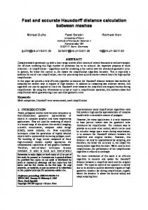
1. Sort the rank intervals of u by the x-coordinate of the intersection with the reference segment of u. 2. For the resulting ordered sequence compute the prefix-maxima of the highest ranks and the prefix-minima of the lowest ranks. 3. Replace the i-th interval [ri,1 , ri,2 ], i = 2, 3, . . . , by two intervals [ri,1 , mini−1 −1] and [maxi−1 +1, ri,2 ], where mini−1 = mink=1,...i−1 rk,1 and maxi−1 = maxk=1,...i−1 rk,2 (see Fig. 4). 4. Discard all empty intervals, i.e., intervals [r1 , r2 ] where r2 < r1 . The prefix-minimum (mini ) and the prefix-maximum (maxi ) for the i-th interval in the ordered sequence from Step 3.3 give us the range of ranks of the red segments that are already intersected by at least one of the corresponding blue segments b1 , . . . , bi before they (possibly) encounter an intersection with the segment bi+1 . Thus, we can remove the [mini , maxi ] interval from the interval of bi+1 . After the interval spliting and shrinking TI (v) is no longer an interval tree, but the remaining intervals have the following properties: The rank intervals stored in one node of TI (v) are now disjoint, i.e., the rank of every segment a ∈ CA (v) is contained in at most one interval of a single node. The number of intervals in TI (v) is at most twice the original number. Since every rank is stored in at most one node of each level of TI (v), the rank of every a ∈ CA (v) is contained in at most O(log n) intervals in TI (v). An example of such interval reduction for one node of the interval tree TI (v) is given in Figure 4. a7 a6

a7 a6 b2

b2

a5 a4 a3 a2 a1

b3

b5

b1 b4 v

a5 a4 a3 a2 a1

b3

b5

b1 b4 v

b1 b2 b3 b4 b5

rank interval [2, 4] [4, 5] [3, 4] [1, 6] [2, 7]

prefixmin 2 2 2 1 1

prefixmax 4 5 5 6 7

new interval(s) [2, 4] [5, 5] empty [1, 1], [6, 6] [7, 7]

Figure 4: Segments in CA (v) and EB (v) corresponding to one node of TI (v) with the reference rank 4. In the right picture the removed parts of the intervals are denoted by dashed lines. Finally, we can reorganize TI (v) and compute the intersection points: Step 3.4. For each node v ∈ T in parallel rebuild the interval tree TI (v) for the new intervals. Step 3.5. For each red segment a ∈ CA (v) in parallel find all b ∈ EB (v) whose intervals in TI (v) contain the rank of a. Record the intersection point with the minimal x-coordinate. 9

The last step is to select the intersection points to report from the candidate intersections: Step 4. Sort the candidate intersection points computed in Steps 2 and 3 lexicographically by (ai ,x-coordinate), where ai is an identifier of the red segment in A. For each a ∈ A report the intersection point with the minimal x-coordinate. In the next section we prove that the described algorithm correctly reports the first intersections of each segment in A and do the counting to show the workload claimed in Theorem 1.

4

Proof of Theorem 1

The correctness of the algorithm is based on the fact that in Steps 2 and 3 of the algorithm we consider all types of possible intersections and for each segment a ∈ A discard only such intersections of each type which cannot have the minimal x-coordinate. We elaborate on the latter claim: Consider the intersections of type (1) and (2), i.e., intersections within the vertical slab of a node v of T of a segment a in CA (v) or in EA (v) with the segments in CB (v), which are handled in Step 2 of the algorithm. Since there are no blue-blue intersections, the segments of CB (v) partition the vertical slab corresponding to the x-interval of v into (curvilinear) quadrilaterals. By locating the neighbors of a in CB (v) at the leftmost point of a within the vertical slab of v we find the quadrilateral in which a “enters” the slab of v. Clearly, the first intersection for a within the slab of v (if any exists) is with one of its blue neighbors. Because all curve segments are x-monotone, this is also the intersection with the lowest x-coordinate within the interval of v. We can safely discard all further intersections of a with CB (v). In Step 3 we initially capture all intersections of type (3) in the rank intervals without explicitly computing each intersection. Since our curve segments are well-behaved and we split the blue segments into subsegments that intersect each red curve at most once, if two blue sub-segments intersect both two red segments a1 and a2 , then the x-order of their intersection points is the same for a1 and a2 . Thus, when we exclude the rank of a red segment a from the interval of a blue sub-segment b in Step 3.3, we know that there is another blue subsegment, whose intersection with a has a lower x-coordinate. The intersection of a and b can then safely be discarded. Next we prove the running time and the resource usage of the algorithm claimed in Theorem 1: Step 1 can be performed in O(log n) time on O(n) processor CREW-PRAM, see [1]. A segment tree uses O(n log n) space. In Step 2 we assign to each segment a ∈ A a processor which traverses the segment tree T and for each node v, with a ∈ CA (v) ∪ EA (v) performs a binary search on CB (v) to determine the neighbors of a. The intersection computation is performed in constant time. This gives us O(log n) time for each of the O(log n) levels of T , i.e., O(log2 n) time with O(n) processors for

10

all candidate intersections of type (1) and (2). Alternatively, we could assign a processor to each occurrence of a segment a in cover- and end-lists of T and find all candidates of type (1) and (2) in O(log n) time using O(n log n) processors. The first variant gives us O(n) candidate intersections in Step 2, the second – O(n log n). In Step 3.1 using one processor for each b ∈ B we can find in time O(log2 n) all rank intervals for the intersections of type (3) in T . Since each b occurs in the end lists of at most two nodes per level of the segment tree T , each b produces O(log n) such intervals. Sorting all O(n log n) boundaries of the rank intervals lexicographically by (v, r), where v is the node of T that produced the interval, and r is a boundary of the interval, we get the grouping of the intervals by the nodes of T and sorting the interval boundaries in one step. This sorting can be performed in O(log2 n) time using O(n) processors. Within the same time and processor bounds we can construct all interval trees in parallel (Step 3.2). Since an interval tree uses linear storage, the total space requirements remain O(n log n). The operations in Step 3.3 involve sorting lists with a total number of O(n log n) elements, and performing prefix-max and prefix-min computations on these lists. These operations stay within the stated resource bounds. Splitting of the intervals and eventually deleting some of them can be performed independently for each interval, i.e., in O(log n) time by O(n) processors in total. The number of the intervals is at most doubled in Step 3.3, thus the storage requirement remains O(n log n) and Step 3.4 has the same resource requirements as Step 3.2. In Step 3.5 using one processor for each red segment a we can traverse the segment tree T and in each node v, such that a ∈ CA (v) find all intervals in TI (v) that contain the rank of a in CA (v). As mentioned above, there are at most O(log n) such intervals in TI (v). Each interval corresponds to a blue segment in EB (v). Instead of reporting all intervals we compute the intersection of a with the corresponding blue segment and keep track of the intersection point with minimal x-coordinate. The computation of all intersection points of a stored in TI (v) is performed in O(log n) time, which gives us total of O(log2 n) time over all levels of T . The number of candidate intersections produced in Step 3 is O(n) – at most one for each red segment. Alternatively, all operations of Step 3 can be performed in O(log n) time on O(n log n) processors. In Step 4 we sort O(n) candidate intersection points by (a, x), where a is the number of the red segment and x is the x-coordinate of the intersection point, and take the minimum for each red segment. Step 4 can be performed in O(log n) time using O(n) processors. Which concludes the proof of Theorem 1. Throughout the algorithm we clearly use concurrent read operations, but for each write operation for each processor we can independently determine a unique storage slot. Thus the algorithm is designed for the CREW-PRAM model.

11

5

Concluding Remarks

The algorithm presented here can further be accelerated to perform Step 2 in O(log n) time using O(n) processors by applying the fractional cascading technique [8], [5]. This technique simplifies the iterative search for a key in multiple ordered lists and allows to perform the search of a segment a in all CB -lists of T in O(log n) time, i.e., taking O(log n) time on O(n) processors for Step 2. Steps 1 and 4 have already these time and processor bounds. But it is not clear whether the performance of Step 3 can be improved. A further interesting related problem is matching geometric shapes under transformations (e.g., translations, rotations, scalings) with respect to the Hausdorff distance, i.e., find a transformation of one of the shapes such that the Hausdorff distance is minimized, for sequential algorithms see [2]. Another interesting distance measure is the Frech´et distance [3]. A parallel solution to the decision problem, i.e., testing whether the Frech´et distance between two polygonal curves is at most some given value ε, should be uncomplicated, since the sequential algorithm uses divide-and-conquer technique. We are currently working on a parallel algorithm for the computation problem, for which the sequential algorithm uses parametric search.

References ´ unlaing, and C. Yap. Parallel [1] A. Aggarwal, B. Chazelle, L. Guibas, C. O’D´ computational geometry. Algorithmica, 3(1):293–327, 1988. [2] H. Alt, B. Behrends, and J. Bl¨omer. Approximate matching of polygonal shapes. Annals of Mathematics and Artificial Intelligence, 13:251–265, 1995. [3] H. Alt and M. Godau. Computing the Fr´echet distance between two polygonal curves. Internat. J. Comput. Geom. Appl., 5:75–91, 1995. [4] H. Alt and L. Scharf. Computing the Hausdorff distance between curved objects. Int. J. Comput. Geometry Appl., 18(4):307–320, August 2008. [5] M. J. Atallah, R. Cole, and M. T. Goodrich. Cascading divide-and-conquer: a technique for designing parallel algorithms. SIAM J. Comput., 18(3):499– 532, 1989. [6] J. L. Bentley and D. Wood. An optimal worst case algorithm for reporting intersections of rectangles. IEEE Trans. Comput., 29(7):571–577, July 1980. [7] B. Chazelle. Intersecting is easier than sorting. In STOC ’84: Proceedings of the sixteenth annual ACM symposium on Theory of computing, pages 125–134, New York, NY, USA, 1984. ACM.

12

[8] B. Chazelle and L. J. Guibas. Fractional cascading: I. a data structuring technique. Algorithmica, 1:133–162, 1986. [9] M. de Berg, O. Cheong, M. van Kreveld, and M. Overmars. Computational Geometry. Springer, Berlin, third edition, 2008. [10] M. T. Goodrich. Intersecting line segments in parallel with an outputsensitive number of processors. In Proceedings of the first annual ACM symposium on Parallel algorithms and architectures, SPAA ’89, pages 127– 137, New York, NY, USA, 1989. ACM. ´ unlaing, and C.-K. Yap. Constructing the voronoi [11] M. T. Goodrich, C. O’D´ diagram of a set of line segments in parallel. Algorithmica, 9(2):128–141, 1993. [12] M. T. Goodrich, S. B. Shauck, and S. Guha. Parallel methods for visibility and shortest path problems in simple polygons (preliminary version). In Proceedings of the sixth annual symposium on Computational geometry, SCG ’90, pages 73–82, New York, NY, USA, 1990. ACM. [13] F. P. Preparata and M. I. Shamos. Computational geometry: an introduction. Springer-Verlag New York, Inc., New York, NY, USA, 1985. [14] R. Tamassia and J. S. Vitter. Optimal parallel algorithms for transitive closure and point location in planar structures. In Proceedings of the first annual ACM symposium on Parallel algorithms and architectures, SPAA ’89, pages 399–408, New York, NY, USA, 1989. ACM.

13