49th AIAA/ASME/ASCE/AHS/ASC Structures, Structural Dynamics, and Materials Conference
16t 7 - 10 April 2008, Schaumburg, IL
AIAA 2008-1814
Computational Aeroelasticity Framework for Analyzing Flapping Wing Micro Air Vehicles Satish Kumar Chimakurthi*1, Jian Tang*2, Rafael Palacios**3, Carlos E. S. Cesnik*4, and Wei Shyy*5 *Department of Aerospace Engineering University of Michigan, Ann Arbor, MI, 48109, U.S.A. **Department of Aeronautics Imperial College, London, SW7 2AZ, U.K. Due to their small size and flight regime, coupling of aerodynamics, structural dynamics, and flight dynamics is critical for Micro Aerial Vehicles. This paper presents a computational framework for simulating structural models of varied fidelity and a Navier-Stokes solver, aimed at simulating flapping and flexible wings. The structural model utilizes either (i) the in-house developed UM/NLABS, which decomposes the equations of 3-D elasticity into cross-sectional and spanwise analyses for slender wings; or (ii) MSC.Marc, which is a commercial finite element solver capable of modeling geometrically-nonlinear structures of arbitrary geometry. The flow solver employs a well tested pressure-based algorithm implemented in STREAM. A NACA0012 cross-section rectangular wing of aspect ratio 3, chord Reynolds number of 3x10⁴, and reduced frequency varying from 0.4 to 1.82 is investigated. Both rigid and flexible wing results are presented and good agreement between experiment and computation are shown regarding tip displacement and thrust coefficient. Issues related to coupling strategies, fluid physics associated with rigid and flexible wings, and implications of fluid density on aerodynamic loading are also explored in this paper.
Nomenclature a root
plunge amplitude
c
mean aerodynamic chord length
CT
thrust coefficient
CL
lift coefficient
D
plate bending stiffness
f
frequency (Hz)
f0, f1
beam forces per unit length; first-order forces per unit length associated to the work needed to deform the cross-section
fs0, fs1
generalized forces corresponding to the finite section modes
FB
beam sectional forces expressed in the deformed frame
h
displacement at a point along y-axis
__________________________ Graduate Research Assistant,
[email protected], Member AIAA. 2 Post-doctoral Fellow,
[email protected], Member AIAA. 3 Lecturer,
[email protected], Member AIAA. 4 Associate Professor,
[email protected], Associate Fellow AIAA. 5 Clarence L. “Kelly” Johnson Collegiate Professor and Chair,
[email protected], Fellow AIAA. 1
1 American Institute of Aeronautics and Astronautics Copyright © 2008 by Satish Kumar Chimakurthi, Jian Tang, Rafael Palacios, Carlos E. S. Cesnik, and Wei Shyy. Published by the American Institute of Aeronautics and Astronautics, Inc., with
a root c
hr
non-dimensional plunge amplitude =
HB
angular momentum column-matrix expressed in the deformed structural frame
k
reduced frequency =
K
kinetic energy per unit length
m0 ,m1
beam moments per unit length, first-order moments per unit length associated to the work needed to deform cross-section
M
cross-sectional inertia matrix
MB
beam sectional moments expressed in the deformed frame
MB
beam sectional moments expressed in the deformed frame
p
static pressure
PB
linear momentum column-matrix expressed in the deformed frame
q
amplitude of the finite-section mode
q’
derivative of the finite-section mode along the spanwise direction
Qs0
generalized forces corresponding to finite-section modes
Qs1
generalized moments corresponding to finite-section modes
Qt
generalized momenta corresponding to finite-section modes
Re
Reynolds number = ρUc
ωc 2U
μ
S
cross-sectional stiffness matrix
St
Strouhal number = hr k
t
time
t
non-dimensional time = tU c
T
plunge cycle period
ui
fluid velocity vector components
U
free stream velocity
U
strain energy per unit length
VB
beam inertial velocity column-matrix at the deformed frame
w
column-matrix of 3-D warping displacements components
x,y,z
global cartesian coordinates
x, x1
coordinate along the structural wing span
x2 , x3
coordinates in the wing cross section 2 American Institute of Aeronautics and Astronautics
αinst
instantaneous effective angle of attack
γ
column matrix of force strains measures
κ
column matrix of moment strain measures
μ
dynamic viscosity
μB
components of the applied generalized forces in the deformed frame
ξB
column matrix of normalized cross section coordinates
π1
ratio of elastic and aerodynamic forces =
π2
ratio of inertia and aerodynamic generalized forces =
π3
ratio of the first bending mode to the frequency of oscillation
π4
ratio of the second bending mode to the frequency of oscillation
π5
ratio of the first torsion mode to the frequency of oscillation
ρf
fluid density
ρm
material volumetric density
ρs
equivalent structural volumetric density
ω
angular frequency = 2π f
ΩB
inertial angular velocity vector at a point on the beam reference line in the deformed frame
D
ρ f U 2 c3 IB
ρ f c5
Superscripts • non-dimensional quantities •′ differentiation with respect to the coordinate along the spanwise direction, x1 •& differentiation with respect to time
I.
Introduction
M
icro Air Vehicles (MAVs) are advancing our capabilities in the areas of environmental monitoring and homeland security [1]. Due to their small size and flight regime, the coupling between aerodynamics, structural dynamics, and flight dynamics is critical. MAVs have a maximum dimension on the order of 15 cm and nominal flight speeds of approximately 10 m/s, operating in a low Reynolds number regime (105 or lower). The rise and growth of MAVs have been stimulated by the long history of natural flight studies. Good reviews of the state-of-the-art in this subject are given in Refs. [2] and [3]. High speed cine and still photography and stroboscopy indicate that most biological flyers undergo orderly deformation in flight [4]. Birds, bats, and insects exploit the coupling between flexible wings and aerodynamic forces such that the wing deformations improve aerodynamic performance [5]. The interaction between unsteady aerodynamics and structural flexibility is, therefore, of considerable importance for MAV development [1]. Much of the aeroelasticity efforts thus far have focused on fixed wing membrane-based MAVs [6-10]. Shyy et al. [6] have discussed flexible wings utilizing membrane materials and inferred from computations that compared to a 3 American Institute of Aeronautics and Astronautics
rigid wing, a membrane wing can adapt to stall better and has the potential to achieve enhanced agility and storage condition by morphing its shape. They also emphasized the importance of fluid-structure analyses to understand the membrane wing performance. Lian and Shyy [7] have studied the three-dimensional interaction between a membrane wing and its surrounding fluid flow via an aeroelastic coupling of a nonlinear membrane structural solver and a Navier-Stokes solver. Stanford et al. [8] made a direct comparison of wing displacements, strains, and aerodynamic loads obtained via a novel experimental setup with those obtained numerically. In their work, they considered both pre- and post-stall angles of attack and the computed flow structures revealed several key aeroelastic effects: decreased tip vortex strength, pressure spikes and flow deceleration at the tangent discontinuity of the inflated membrane boundary, and an adaptive shift of pressure distribution in response to aerodynamic loading. The aeroelasticity of flapping wings has only recently been seriously addressed and a full picture of the basic aeroelastic phenomena in flapping flight is still not clear [1, 5, 11-21]. In an earlier investigation, Smith [14] has studied the effects of flexibility on the aerodynamics of Moth wings by modeling them as linearly elastic structures using finite elements for a Reynolds number of the order of 103 and reduced frequencies of the order of 0.2 and higher. Laminar flow assumption was made. In the structural finite element model, the veins of the wings were treated as tubular beams of varying thickness, and the wing surfaces were modeled as quadrilateral (or triangular) membranes that are also of varying thickness with orthotropic properties. For the aerodynamics, an unsteady panel method was used. Both the structural and the aerodynamic equations were simultaneously solved to obtain the coupled flapping wing response. Frampton et al. [5] have investigated a method of wing construction that results in an optimal relationship between flapping wing bending and twisting such that optimal thrust forces are generated. The thrust production of flapping wings was tested in an experimental rig. Results from this study indicated that the phase between bending motion and torsional motion is critical for the production of thrust. It was noted that a wing with bending and torsional motion in phase creates the largest thrust whereas a wing with the torsional motion lagging the bending motion by 90 deg results in the best efficiency. Hamamoto et al. [15] have done finite element analysis based on the arbitrary Lagrangian-Eulerian method to perform fluid-structure interaction analysis on a deformable dragonfly wing in hover and examined the advantages and disadvantages of flexibility. They tested three types of flapping flight: a flexible wing driven by dragonfly flapping motion, a rigid wing (stiffened version of the original flexible dragonfly wing) driven by dragonfly flapping motion, and a rigid wing driven by modified flapping based on wing tip motion. They found that the flexible wing with nearly the same average energy consumption generated almost the same amount of lift force as the rigid wing with modified flapping motion. In this case, the motion of the tip of the flexible wing provided equivalent lift as the motion of the root of the rigid wing. However, the rigid wing required 19% more peak torque and 34% more peak power, indicating the usefulness of wing flexibility. More recently, Singh [11] has discussed a computational framework for the aeroelastic analysis of hovercapable, bio-inspired flapping wings. The chord-based Reynolds number considered for the analyses was in the 103 to 105 range. A finite element-based structural analysis of the wing was used along with an unsteady aerodynamic analysis based on indicial functions. Experimental validation of the computational results was conducted. One of the major inferences from this work is that at high flapping frequencies (~ 12 Hz), the light-weight and highly flexible insect-like wings used in the study exhibited significant aeroelastic effects. Zhu [16] has developed a nonlinear fluid-structure interaction approach to study the unsteady oscillation of a flexible wing for a Reynolds number of 2.025 x 10⁴. His hybrid solution approach included a three-dimensional boundary-integral method to solve the flow around the body and the dynamics of the wake, and a nonlinear thin-plate model to simulate the structural response of the wing. He found that when the wing is immersed in air, the chordwise flexibility reduces both the thrust and the propulsion efficiency and the spanwise flexibility (through equivalent plunge and pitch flexibility) increases the thrust without efficiency reduction within a small range of structural parameters. However, when the wing is immersed in water, the chordwise flexibility increased the efficiency and the spanwise flexibility reduced both the thrust and the efficiency. Wills et al. [17] have presented a computational framework to design and analyze flapping MAV flight. A series of different geometric and physical fidelity level representations of solution methodologies was described in the work. Liani et al. [18] have coupled an unsteady panel method with Lagrange's equations of motion for a two degree-of-freedom (2-DOF) spring-mass wing section system to investigate the aeroelastic effect on the aerodynamic forces produced by a flexible flapping wing at different frequencies especially near its resonance. Heathcote et al. [19] have experimentally investigated the effects of stiffness on thrust generation of airfoils undergoing a plunging motion under various free stream velocities. Direct force measurements showed that the thrust/input-power ratio was found to be greater for flexible airfoils than for the rigid one. They also observed that at high plunging frequencies, the less flexible airfoil generates the largest thrust, while the more flexible airfoil generates the most thrust at low frequencies. To study the effect of the spanwise stiffness on the thrust, lift and 4 American Institute of Aeronautics and Astronautics
propulsive efficiency of a plunging wing, a water tunnel study was conducted by them on a NACA0012 uniform wing of aspect ratio 3. They observed that for Strouhal numbers greater than 0.2, a degree of spanwise flexibility was found to be beneficial. Tang et al. [20] explored a two-dimensional flexible airfoil by coupling a pressure based fluid solver with a linear beam solver. In this work, the fluid flow around a plate of different thicknesses with a teardrop shaped leading edge was computed at a Reynolds number of 9x10³. In addition to this, a flat plate with half cylinders at leading and trailing edges were investigated at a Reynolds number of 102 to probe the mechanism of thrust generation. In particular, they pointed out that the effect of the deformation (passive pitching) is similar to the rigid body motion (rigid pitching), meaning that the detailed shape of the airfoil is secondary to the equivalent angle of attack. This paper is part of an ongoing study in the computational aeroelasticity of flapping wings. Previously [21] a fluidstructure coupling procedure between a Navier-Stokes solver and a quasi-three-dimensional finite element solver was introduced. Results were presented on a model example problem corresponding to a NACA0012 wing of aspect ratio 3 in pure heave motion at a Reynolds number of 3x10⁴. It was observed that the phase lag of the wing tip displacement relative to the flapping motion becomes more pronounced as the fluid density increases. The main objectives of this paper are to: a) present computational aeroelastic frameworks for the analysis of flapping wings; b) validate the proposed computational methodology for the aeroelasticity of flapping wings with the experimental results of Heathcote et al. [19]; and c) study the characteristics of the coupling between fluid and structural dynamics solvers, the impact of aerodynamic loading on the structural response, the implications of the thrust coefficient in response to the reduced frequency, and the fluid physics associated with flexibility.
II. Numerical Framework for High-Fidelity Flapping Wing Simulations In this section, a brief description of the fluid dynamics formulation and two structural dynamics approaches for the problem of geometrically nonlinear deformations of flapping wings is presented. From these, two aeroelastic frameworks are developed for the analysis of low Re flows and their interactions with flexible flapping wings. Computational Fluid Dynamics Solution (STREAM) The fluid solution is obtained from the incompressible Navier-Stokes equations and the continuity equation ∂u i ∂t ∂u i ∂x i
+
∂ ∂x j
(u j u i ) = −
1
∂p
ρ f ∂x i
+υ
2 ∂ ui 2 ∂x j
(1)
=0
where ρ f is the fluid density, ui is the velocity vector, t is the time, xi is the position vector, p is the pressure, and υ is the kinematic viscosity. Based on the definition of the motion [20] for forward flight, if the free stream velocity (U), the chord length (c) and the inverse plunging/pitching (1/f) frequency are used as the velocity, length, and time scales respectively, the Reynolds and Strouhal numbers appear as Re = Uc / ν , and St = fc / U . With these choices of the scaling parameters, the non-dimensional form of the Navier-Stokes equations becomes: St
1 ∂ 2 ui ∂ ∂ ∂p (ui ) + (u j ui ) = − + ∂t ∂x j ∂xi Re ∂x j2
(2)
It should be noted that the relation between Strouhal number and reduced frequency is St = hr k . The numerical solution is obtained using a pressure-based algorithm, with an employment of combined cartesian and contravariant velocity variables to facilitate strong conservation law formulations and consistent finite volume treatment. The convection terms are discretized using a second-order upwind scheme, while the pressure and viscous terms with a second-order central difference scheme. For the time integration, an implicit Euler scheme is employed. A moving grid technique employing the master-slave concept [7] is used to re-mesh the multi-block structured grid for fluidstructure interaction problems. The geometric conservation law (GCL) originally proposed by Thomas and Lombard [22] was incorporated to compute the cell volumes in the moving boundary problem consistently and eliminate 5 American Institute of Aeronautics and Astronautics
artificial mass sources. The specific implementation and implications of the GCL in the context of the present solution algorithm have been discussed by Shyy et al. [23]. Structural Dynamics Solution (UM/NLABS) The first geometrically-nonlinear structural dynamic solution is based on an asymptotic approach to the equations governing the dynamics of a general 3-D anisotropic slender solid [24, 25]. It is implemented in the University of Michigan’s Nonlinear Active Beam Solver (UM/NLABS) computer code. Assuming the presence of a small parameter (the inverse of the wing aspect ratio) allows for a multi-scale solution process, in which the problem is decomposed into separate cross-sectional (small-scale) and longitudinal (long-scale) analyses. The longitudinal problem solves for average measures of deformation of the reference line under given external excitations. The cross-sectional problem solves the local deformation for given values of the long-scale variables. Both problems are tightly coupled and together provide an efficient approximation to the displacement field in the original 3-D domain. A flow diagram of the process is shown in Figure 1. The structural formulation follows the variational-asymptotic method for the analysis of composite beams [26]: the equations of motion for a slender anisotropic elastic 3-D solid are approximated by the recursive solution of a linear 2-D problem at each cross section [25], and a 1-D geometrically-nonlinear problem along the reference line [24]. This procedure allows the asymptotic approximation of the 3-D warping field in the beam cross sections, which are used with the 1-D beam solution to recover a 3-D displacement field. The warping was approximated for the elastic degrees of freedom of a Timoshenko-beam model (extension and transverse shear, γ, and twist, bending about two directions, κ) and augmented with an arbitrary set of functions approximating the sectional deformation field (amplitude, q, and its derivative along the spanwise direction, q ′ ). These capture “non-classical” deformations, which are referred to as finite-section modes. And these new deformation modes are not restricted to be as small as the fundamental warping field. The solution of a variational problem yields the warping field corresponding to 1-D beam strains {γ ,κ ,q,q′} . In its first order approximation, it can be written as [25]
w(x1 ,x2 ,x3 ) = wγ (x2 ,x3 )γ (x1 ) + wκ (x2 ,x3 )κ (x1 ) + wqn (x2 ,x3 )qn (x1 ) + wqn′ (x2 ,x3 )qn′ (x1 ) + H .O.T . ,
{
where wγ wκ wqn wqn′
(3)
} are the first-order warping influence coefficients. Using this approximation for the warping
field, the cross-section problem gives the strain energy per unit length of the beam:
U=
{
1 T γ 2
κT
qT
q ′T
}
⎧γ ⎫ ⎪κ ⎪ [ S ] ⎪⎨ q ⎪⎬ + H .O.T . ⎪ ⎪ ⎪⎩q ′⎪⎭
(4)
Here, the constant matrix [S] is the first-order asymptotic approximation to the stiffness matrix. The integration of the kinetic energy can be directly done as function of the 1-D variables, yielding:
{
1 K = VBT 2
ΩTB
q&n
T
}
⎧ VB ⎫ [ M ] ⎪⎨Ω B ⎪⎬ , ⎪ ⎪ ⎩ q&n ⎭
(5)
where the constant matrix [M] is the inertia matrix for the cross section. From the resulting 1-D problem, the geometrically-nonlinear dynamic equations of equilibrium along the reference line (as presented in Ref. 24) are written as
( dtd + Ω% B ) PB = ( dxd + K% B ) ( FB − f1 ) + f0 , ( dtd + Ω% B ) H B + V%B PB = ( dxd + K% B ) ( M B − m1 ) + (e%1 + γ%)FB + m0 , d dt
Qt =
d dx
(Q
s1
) (
)
− f s1 − Qs0 − f s0 .
6 American Institute of Aeronautics and Astronautics
(6)
where the generalized forces and momenta are all expressed in their components in a reference frame attached to the deformed beam reference line. The first two equations imply equilibrium of forces and moments. The last equation in (6) includes the set of equilibrium equations corresponding to the finite-section modes. With the warping influence coefficients given by Eq. (3), the applied forces per unit length in Eq. (6) are f 0 = ∫ μ B dA, f1 = ∫ wγT μ B dA, A(x )
f s0 = ∫
A(x )
(
ΨTq
+ wqT
)μ
A (x )
f s1 = ∫ wqT′ μ B dA, ,.
B dA, ,
A(x )
m0 = ∫ ξ B μ B dA,
(7)
m1 = ∫ wκ μ B dA. T
A (x )
A(x )
The present implementation of this formulation follows the approach described in Ref. 24, where the solution to Eq. (6) is done by means of a finite-element discretization on a mixed-variational form of the equations. Therefore, although they are analyzed independently, the small and long-scale problems are intimately linked in the detailed approximation to the solution. This is particularly important in the generation of the solid side of an aeroelastic model: the interface of the structural model consists of the actual wetted surfaces of the vehicle, without extrapolations from the motion of a reduced-dimension structural model, nor the assumption of rigid cross sections required by beam theories.
Cross-sectional geometry and material distribution 1-D Kinematic variables
Warping Influence Coefficients
Cross-sectional analysis
Stiffness Inertia
1-D geometrical definition
Geometricallynonlinear 1-D analysis
1-D strains and displacements
Sectional forces
External loads 3-D domain assembler Time domain 3-D displacements
Fig 1. Asymptotic solution process for 3-D slender structures implemented in UM/NLABS Structural Dynamics Model (MSC.Marc 2005r3) The ability to model very-flexible low-aspect-ratio flapping wings made of anisotropic materials is ultimately required to analyze and design bio-inspired wings. MSC.Marc [27] is a commercial nonlinear finite-element solver that can be used toward this end. It is capable of handling nonlinearities either due to material behavior, large deformation, or boundary conditions. It contains three isoparametric, doubly curved, thin shell elements: 3-, 4-, and 8-node elements based on Koiter-Sanders theory [27]. These elements are C 1 continuous and exactly represent rigid-body modes, critical in flapping wing analyses. Some of the shell elements in the solver could be used in conjunction with selected beam elements to model build-up structural wing constructions. MSC.Marc provides a coupling interface to external CFD solvers available through user subroutine programming. Such an interface was developed in this work to perform aeroelastic simulations.
7 American Institute of Aeronautics and Astronautics
Aeroelastic Coupling The aeroelastic coupled solution is based on a time-domain partitioned solution process in which the nonlinear partial differential equations modeling the dynamic behavior of both fluid and structure are solved independently with boundary information (aerodynamic loads and structural displacements) being shared between each other alternately. A schematic of such a framework is shown in Figure 2. A dedicated interface module was developed to enable communication between the flow and the structure at the 3-D wetted surface (fluid-structure interface). In the interface module, both the fluid and the structural modules are called one after the other according to the coupling method adopted for the problem. The coupling algorithm is determined by the capability of the individual simulation code.
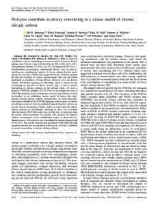
There are two coupling algorithms within the purview of the aeroelasticity frameworks proposed here. In the first one, denoted here as the explicit coupling approach, both solvers are called once per coupled time-step while exchanging data at the interface. In the second algorithm, denoted here as the implicit coupling approach, both the fluid and the structural solvers exchange more than once per coupled time-step (see Figure 3). The number of such fluid-structure subiterations is determined by a specified convergence criterion. Between any two fluid-structure subiterations, the initial conditions in the solvers are not updated and hence a new solution is obtained for the same time-step at the end of a subiteration. However, between the last fluid-structure subiteration of a coupled time-step and the first fluid-structure subiteration of the subsequent coupled time-step, the initial conditions in the solvers are updated and the solution is time-marched. It is important to note that numerical instabilities have been encountered [28] due to added-mass effects when explicit coupling methods were used to study the interaction of thin-elastic structures with incompressible, viscous flows. Such algorithms exhibit numerical instabilities for a given geometry as soon as the density of the structure is lower than a certain threshold.
Fig 2. A schematic of the aeroelastic framework involving Navier-Stokes and two different structural solvers of variable fidelity Two separate coupled simulation codes have been developed for this work. The first is between UM/NLABS and STREAM and the second is between MSC.Marc and STREAM. Both explicit and implicit coupling algorithms have been adopted for the simulation code involving UM/NLABS. Only the explicit method was possible in the case of the code involving MSC.Marc since the code does not support exchanges with the external CFD solver within a coupled time-step.
For the development of the coupled simulation codes, several interface subroutines have been written to control the coupled solution and to perform interpolation of physical quantities between the fluid and the structural grids via thin-plate spline [29] or bilinear interpolation methods. A coupled code was achieved simply by compiling the object files of the individual solvers along with those of the interface routines to produce a shared executable. 8 American Institute of Aeronautics and Astronautics
Considering the limitations of the explicit coupling approach as discussed above, only the implicit coupling was applied in the simulations involving UM/NLABS in this work.
Fig 3. A schematic of the implicit coupling approach involving fluid-structure subiterations
III. Results and Discussion This section is divided into three subsections. In the first one, a brief description of the test problems that are considered in this study is provided. In the second subsection, details of the fluid and the structural computational models are provided. Finally in the third subsection, computational results on a rectangular wing configuration of NACA0012 cross-section (both rigid and flexible) are reported and compared against the experimental results of Heathcote et al. [19]. A. Description of the Validation Case In an attempt to validate the proposed coupled fluid-structure frameworks, results were obtained on a threedimensional rectangular wing of NACA0012 uniform cross section oscillating in water in pure heave. Water tunnel studies have been performed by Heathcote et al. [19] to study the effect of spanwise flexibility on the thrust, lift, and propulsive efficiency on this configuration. A schematic of the experimental setup is shown in Figure 4. Three wings of 0.3-m span and 0.1-m chord with varying levels of flexibility were constructed. The leading edge at the wing root is actuated by a prescribed sinusoidal plunge displacement profile as shown in Figure 5.
Overall wing thrust coefficient and tip displacement response were experimentally measured. Only the “Rigid” and “Flexible” versions of the wings used in the experiment are considered here. The representations of the cross-section constructions are reproduced in Figure 6. B. Computational Models A structured multi-block O-type grid around a NACA0012 wing of aspect ratio 3 was used for the CFD simulations. The number of grid points is 120, 56, and 60 in the tangential, radial and span-wise directions, respectively. Grid sensitivity studies have been performed to identify a grid suitable for the computations in this work. The CFD model setup which includes the boundary conditions is shown in Figure 7 – left.
For the structural representation of the “Rigid” experimental case, the structure was assumed to be infinitely stiff. For the “Flexible” experimental case, two different structural models were developed. The first (Figure 8) is based on a 1-D beam finite-element discretization with 39 elements along the semi-span. Chordwise deformation was reported as being negligible in the experiment, therefore, a beam model with six elastic degrees of freedom, corresponding to extension, twist, and shear and bending in two directions, was chosen. The beam reference line (cantilevered to a plunging frame of reference) is chosen along the leading edge of the wing (highlighted in black in Figure 8 - bottom) and cross-sectional properties are evaluated with respect to the leading edge point. Furthermore, the properties are uniform throughout the semi-span. The contribution of the PDMS rubber material (used in the experimental wing configuration) to the overall mass and stiffness properties was found to be negligible; therefore, only the stainless steel stiffener (rectangular thin strip) was used for the evaluation of cross-sectional properties (Figure 8 - top). The 3-D structural solution is obtained by using 75 recovery nodes on each cross section resulting in a structured grid of 3000 interface points which define the solid side of the aeroelastic interface. The second structural model (Figure 7 - right) is a rectangular plate and it was created in MSC.Marc using four-noded thick shell 9 American Institute of Aeronautics and Astronautics
elements (MSC.Marc element number 75). The wing is actuated by prescribing motion to a pivot point which is connected to the structure via a rigid link.
Fig 4. Water-tunnel experimental setup (from Heathcote et al. [19])
Fig 5. Prescribed plunge motion for the rectangular wing (normalized w.r.t. amplitude) (Points A, B, C, and D are representative time instants corresponding to 0, T/4, T/2, and 3T/4, respectively, and are used at several places in this document for referencing purposes)
Fig 6. (i) Rigid and (ii) Flexible wing cross-sections used in the experiments of Heathcote et al. [19]
10 American Institute of Aeronautics and Astronautics
Fig 7. CFD computational model setup for the rectangular wing (left), Shell finite element model of the thinrectangular steel strip in MSC.Marc (right)
A summary of the wing geometrical and mechanical properties is included in Table 1. Table 2 provides information about the flow properties (dimensional). In Table 3, all dimensionless numbers related to either the structure, the flow, or to both are furnished. The dimensionless numbers π 1 , π 2 , π 3 , π 4 , and π 5 are discussed in more detail in Ref. 31. Table 1. Geometric and mechanical properties of the wing Semi-span 0.3 m Structural thickness Chord 0.1 m Density of steel Young’s modulus of steel 210 GPa Equivalent structural density
10-3 m 7800 kg/m3 975 kg/m3
Table 2. Flow properties
Flow velocity
0.3 m/s
1.2 kg/m3 1000 kg/m3
Air/Water density
Table 3. Dimensionless parameters associated with wing model Strouhal number Chord-Reynolds number 3x10⁴ Chord-normalized plunge Reduced frequency range 0.40 to 1.82 amplitude
π1 π3 π5
213 5.46 33.7
0.3185 0.175
π2 π4
7.8x10⁻⁸ 34.3
Time step
-3
3x10 , 6x10⁻³, 15x10-3
C. Rectangular wing in pure plunge (rigid and flexible) Computational studies on the “Rigid” and the “Flexible” versions of the wing in the experiments of Heathcote et al. [19] are presented here. Results illustrating numerical issues related to time-step sensitivity, and explicit and implicit coupling methods are discussed first. Next, correlations between computational results and the experimental data are presented. Finally, the effect of structural flexibility on the plunging wing aerodynamics is discussed using pressure distribution and streamlines plotted on the rigid and the flexible wing configurations at selected span stations and at representative time instants.
11 American Institute of Aeronautics and Astronautics
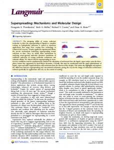
Evaluation of Computational Parameters To assess the independence of the numerical solution to grid refinement, a grid convergence study was performed and a suitable grid was subsequently chosen. This grid has a total of 120, 56, and 60 points in the tangential, radial, and span-wise directions respectively. A time-step sensitivity study was performed with this grid at a reduced frequency of 1.82 and Reynolds number of 3x10⁴. Three different non-dimensional time-steps 3x10⁻³ (1x10⁻³ s), 6x10⁻³ (2x10⁻³ s), and 15x10-3 (5x10⁻³ s), were tested. The corresponding thrust coefficient of the rigid wing as a function of time is shown in Figure 9. Based on this analysis, a time-step of 6x10⁻³ (2x10⁻³ s) was chosen as being adequate to ensure asymptotic convergence and was used in all cases discussed in this paper unless otherwise stated. Explicit and Implicit Coupling Methods To demonstrate the impact of the fluid-structure subiterations within a time-step (implicit computation) on the coupled response, flexible wing computations were performed for a chord Reynolds number of 3x10⁴ and reduced frequency of 1.74 with both explicit and implicit coupling methods. Figure 10 includes the computed lift coefficient response on the wing. In general, there is little difference between the two solutions for the selected time steps. The implicit method, however, eliminates most of the high-frequency error through the forced convergence within each time step, a feature not present in the explicit approach. Therefore, only results based on the implicit coupling method is presented for the UM/NLABS-based solutions, while MSC.Marc ones are based on the explicit method (due to limitations described above).
Figure 11 shows the normalized tip vertical displacement (with respect to the plunge amplitude) for the flexible wing computed with two proposed coupled simulation codes. Good correlation is obtained between the two frameworks and also with the experimental response. This indicates that the frameworks using UM/NLABS (more efficient) and MSC.Marc (more general) work similarly for bend/twist dominated flexible wings and that their integration with the CFD is verified. The MSC.Marc framework will be used to develop complex structural dynamic models of insect wing-like structures for future aeroelastic computations. But for the results that follow, only the UM/NLABS-based framework is used for the studies of this simple wing.
Fig 8. UM/NLABS computational models (rectangular thin-strip cross section used to evaluate structural stiffness and mass properties shown at the top and the CSD-CFD interface grid with the beam reference line indicated in black shown at the bottom) Correlations between Rigid and Flexible Wing Computations with Experiment For the case of chord Reynolds number 3x10⁴ and reduced frequency of 1.82, the thrust coefficient response of both the rigid and flexible wings in pure plunge is shown in Figure 12. The experimental data of Heathcote et al. [19] are also included for comparison. The computational response correlates well with that of the experiment. As found in the experiment, the frequency of the response is twice that of the plunge frequency as the maximum thrust occurs
12 American Institute of Aeronautics and Astronautics
twice in a period as the wing passes through the neutral (zero) position (points B and D of Figure 5). There are, however, missing parts of the troughs corresponding to the rigid wing at the end of downstroke (point C of Figure 5) and both the troughs and the peaks corresponding to the flexible wing at points B and C. The reason for this discrepancy is not clear at this point and will be investigated further. Figure 12 also shows that the thrust coefficient of the flexible wing is greater than that of the rigid wing. This indicates that spanwise flexibility has a favorable impact on the thrust response in the case considered in this paper. It is worth noticing, however, that this result is not universal. As also shown in the experimental studies of Ref. 19, significant flexibility to the wing ( π1 = 71.2 , which is approximately 1/3 of the value for the wing studied here) can reduce the thrust generated when compared to the rigid case. The phase lag associated with structural flexibility affects the effective angles of attack, which means that the specific level and nature of flexibility can affect the outcome of thrust enhancement. Although different in many ways, Ref. 16 also attempts to study the effect of wing flexibility on the thrust generation. Similar result was numerically obtained for a wing with π1 = 57.2 . Simulations were done for both plunge and combined pitch/plunge in water. The author observed from the numerical simulation that the thrust loss is associated with a decrease in heave amplitude along the span of the wing when compared to the prescribed motion. Since the fluid solver used in Ref. 16 is based on a much simplified formulation (boundary element method), its capability to capture certain flow dynamics is questionable (e.g., delayed stall). Limitations like that prevent deeper investigations into the phenomenon. Our proposed aeroelastic framework has the capability of analyzing in great detail the unsteady flow field, which in turn will support the understanding of the fundamental mechanisms behind the thrust generation for different levels of flexibility on flapping wings. This capability is exemplified in the next section. To assess the dependence of thrust production on the reduced frequency of oscillation, a parametric study was conducted on both the rigid and flexible wings. Figure 13 shows the computational results and their comparison with the experiment, showing good correlation between them. As shown from the experiment, the thrust coefficient response increases gradually at low reduced frequencies and more rapidly at higher reduced frequencies. This trend is captured well by the model. It may be noted here that time-steps of 6x10⁻³ (2x10⁻³ s) and 15x10-3 (5x10⁻³ s) were used for the rigid and the flexible wing simulations, respectively. Figure 14 shows the elastic tip deformation response as a function of reduced frequency. Since the experimental results are not readily available, only the computational results are shown. According to them, the amplitude of deformation increases with the oscillation frequency in a similar fashion as the thrust coefficient.
0.8
0.001 s 0.002 s 0.005 s
0.6
C
T
0.4 0.2 0 -0.2 0
0.2
0.4
0.6
0.8
t/T Fig 9. Rigid wing computation (time step sensitivity)
13 American Institute of Aeronautics and Astronautics
1
L
5
0
-5 0
C
C
L
5
0.5
1 t/T
0
Explicit computation Implicit computation
Explicit computation Implicit computation 1.5 2
-5 0
0.1
0.2
0.3
0.4
0.5
t/T
Normalized vertical displacement
Fig 10. Lift coefficient response of the wing for reduced frequency of 1.74 : explicit and implicit coupling methods (left); zoomed view highlighting high frequency oscillations (right)
2
Coupled code (UM/NLABS) Coupled code (MSC.Marc) Experiment
1 0 -1 -2 0
0.2
0.4
0.6
0.8
1
t/T Fig 11. Flexible wing tip displacement response Effect of Structural Flexibility on Aerodynamics To better understand the implications of wing flexibility on the aerodynamics, detailed flow structure and pressure distributions need to be investigated. These are presented here as an illustration of the capability of the proposed aeroelastic framework. Results are shown for selected wing span locations and representative time instants on both the rigid and the flexible wings.
In Figure 15, streamlines (as viewed from the reference frame moving with the prescribed motion) and pressure contours around the airfoil at 50% semi-span location are plotted for both rigid and flexible wings at four different time instants (A,B,C, and D of Figure 5) within a stroke period T. It may be observed from the figure that the streamlines in the case of the flexible wing hit the wing surface because the reference frame with respect to which they were plotted does not take into account the surface speed due to deformation. The following features can be observed: a) At point A (t = 0), i.e., at the beginning of the downstroke, in the case of the rigid wing, a strong vortex is seen on the bottom surface close to the leading edge and a weaker one on the top surface close to the trailing edge. Whereas, in the case of the flexible wing, no vortex is seen on the top surface and the one on the bottom surface is stronger than its counterpart on the rigid wing.
14 American Institute of Aeronautics and Astronautics
b) At point B (t = T/4), i.e., at the middle of the down-stroke, in both rigid and flexible wings, the vortex on the bottom surface becomes weaker and moves downstream. Further, only for the rigid wing, the smaller vortex on the top surface grows in size and also moves downstream towards the trailing edge. This is the point at which maximum thrust is generated in both the rigid and the flexible cases. c) At point C (t = T/2), i.e., at the beginning of the upstroke, in the case of the rigid wing, a large vortical structure is now seen on the top surface closer to the leading edge and a smaller sized vortex on the bottom surface closer to the trailing edge. For the flexible wing, a much stronger vortex is seen on the top surface. d) At point D (t = 3T/4), in the case of the rigid wing, both the vortices seen at time T/2 become weaker and move towards the trailing edge. The one on the top surface moves downstream much less than the one on the bottom. Whereas, in the flexible wing case, the weakening of the vortex is seen but it does not convect downstream as much as its counterpart on the rigid wing. 0.8
Computation Experiment
0.6
C
T
0.4 0.2 0 -0.2 0
0.5
1
1.5
2 t/T
2.5
3
3.5
4
(a) rigid wing
0.8 Computation Experiment
0.6
C
T
0.4 0.2 0 -0.2 0
0.5
1
1.5
2 t/T
2.5
3
3.5
4
(b) flexible wing Fig 12. Time histories of thrust coefficient for both rigid and flexible wings
15 American Institute of Aeronautics and Astronautics
0.4
0.3
0.3
0.2
0.2
C
C
T
T
0.4
0.1
0.1
0
0 -0.1 0
0.5
1 k
Computation Experiment 1.5 2
-0.1 0
0.5
Computation Experiment 1.5 2
1 k
Fig 13. Thrust coefficient as a function of reduced frequency: rigid wing (left), flexible wing (right)
Normalized tip vertical displacement
1.8 1.7 1.6 1.5 1.4 1.3 1.2 1.1 1 0.4
0.6
0.8
1
1.2 k
1.4
1.6
1.8
2
Fig 14. Computed tip elastic vertical deformation normalized with respect to the amplitude of prescribed motion Figure 16 shows the spanwise distribution of pressure contours for both top and bottom surfaces of the rigid and flexible wings corresponding to point B of Figure 5. In general, most of the top surface presents suction for both cases. However, the effect is more pronounced in the case of the flexible wing. Leading edge suction plays a critical role in determining the level of the thrust generated [30]. While the pressure contours presented in Figure 16 provide a global picture of the spanwise variation, in order to focus on the effect of leading edge suction and its enhancement in the case of the flexible wing, Figure 17 shows the pressure field distributions at four stations along the wing semispan (15%, 50%, 83%, 97%) for two different time instants (points B and C of Figure 5). It is seen in the figure that the effect of leading-edge suction is enhanced in the flexible wing case (higher suction peak near the leading edge) which helps explain the increase in thrust with increase in flexibility.
The structural flexibility results in higher instantaneous effective angles of attack, which, in turn, promote larger streamline curvatures around the wing. From the momentum equations, streamline curvatures induce pressure gradients in corresponding manners. The instantaneous effective angle of attack is defined as:
⎛ 1 dh(t ) ⎞ ⎟ ⎝ U dt ⎠
αinst ≡ tan −1 ⎜ −
16 American Institute of Aeronautics and Astronautics
(8)
A
B
C
D Rigid wing Flexible wing Fig 15. Pressure contours and streamlines at four different time instants in a stroke period around the airfoil at 50% semi-span section (as viewed from the reference frame moving with prescribed motion) dh (t ) is the wing velocity component normal to the uniform flow in the case of the rigid wing and, in the dt case of the flexible wing, it is the sum of that and the velocity due to elastic deformation. In order to corroborate the impact of flexibility on thrust generation, Figure 18 shows the time response of the instantaneous angle of attack for both rigid and flexible wings. For the flexible wing case, two different stations along the semi-span (50% and 97%) are considered since each station sees a different effective angle of attack due to wing bending and spanwise variation of velocities induced due to deformation. As seen in the figure, the amplitude of the effective angle of attack in the case of the flexible wing (for 97% semi-span station) is at least 35% higher than that of the rigid wing.
where
17 American Institute of Aeronautics and Astronautics
This reinforces the fact shown in Figure 12 that there is a thrust enhancement due to wing flexibility. Also, it is important to note here that flexible wings can yield favorable performance at quite high instantaneous angles of attack (50 deg) and large streamline curvatures without stalling. In order to discern the effects of flexibility on the flow structure further, streamlines at several stations along the semi-span for both the rigid and the flexible wings are plotted in Figure 19. They are placed next to each other for comparison. These represent the wing when it is at its mean position (point B of Figure 5). The left column corresponds to the rigid wing and the right to the flexible one. Each row in the figure corresponds to a location along From these results, the following observations can be made: •
For the rigid wing, a smaller separation bubble is observed on the top surface near the inboard region of the wing and closer to the wing trailing edge in addition to a bigger one on the bottom surface closer to the leading edge. The smaller bubble is not seen on the flexible wing in any region.
•
On the rigid wing, the separation bubble exists until around 83% semi-span, whereas on the flexible wing, it exists until 60% semi-span. In general, the size of the separation bubble in the case of the flexible wing is smaller than its counterpart on the rigid wing. This may also be observed from the rigid and flexible pressure distributions presented in Figure 16 (bottom surface).
Fig 16. Pressure distribution on the rigid and flexible wings at point B of Figure 5: top surface (left), bottom surface (right) – (magnitudes of pressure are shown in Pa)
•
Figure 19 shows streamlines hitting the wing surface in the case of the flexible wing (similarly to Figure 15). Again, this is because the reference frame with respect to which they were plotted does not take the surface speed due to deformation into account.
Figure 20 includes the elastic tip deformation response (normalized with respect to the plunge amplitude) of the flexible wing in pure plunge (at a constant frequency of oscillation) at two different flow densities (air density, water density) compared to the case in vacuum. The deformation is expressed with respect to a frame that is fixed to the body and moves with the prescribed plunge motion. In both cases, a forward speed of 0.3 m/s was assumed, which fixes the Reynolds number and reduced frequency for the problem. As seen in Figure 20, in the case of the wing oscillating in a fluid of air density, the deformation is almost identical to the case when there are no fluid dynamic forces (vacuum). Ref. 16 reports similar results for a flexible wing in both heave and pitch motion immersed in both air and water. It reports this scenario as being the inertia-driven deformation. The fundamental mechanisms of fluidstructure interaction in different media and for different scaling parameters can now be explored using the proposed framework as exemplified for water here. These studies will be presented in a future paper. 18 American Institute of Aeronautics and Astronautics
15%
50%
83%
97%
t = T/4 (B)
t=T/2 (C)
Fig 17. Pressure field distribution at several stations along the wing semi-span (for time instants corresponding to B and C of Figure 5)
19 American Institute of Aeronautics and Astronautics
Instantaneous angle of attack (deg)
80 Rigid wing Flexible wing (50% semi-span) Flexible wing (97% semi-span)
60 40 20 0 -20 -40 -60 0
0.5
1
1.5
2
2.5
3
3.5
t/T
Fig 18. Time response of the instantaneous angle of attack
Concluding Remarks A computational aeroelastic framework suitable for flapping wing Micro Air Vehicle problems is presented and results from a preliminary validation study are reported. Two structural models of different fidelity levels are presented. The simpler formulation is capable of handling geometrically nonlinear beam-like deformations and linear plate-like motions, and it has been implemented in UM/NLABS, an in-house code. The higher fidelity approach is based on MSC.Marc, a commercial finite element solver capable of modeling geometrically/materially nonlinear shell/plate built-up structures. The Navier-Stokes flow solver employs a well tested pressure-based algorithm, and it is implemented in STREAM. Each of the structural models is independently coupled to the CFD solver resulting in two different coupled simulation codes with distinct capabilities. Based on Heathcote et al.’s experiment, numerical simulations were conducted on a rectangular NACA0012 wing oscillating in pure heave. Quantitatively good agreement with the experimental results was obtained for the thrust coefficient for both rigid and flexible wings in the entire range of reduced frequencies (0.4 to 1.82) considered. Several important conclusions from the numerical studies in this paper are highlighted below: 1) Within the range of non-dimensional parameters considered, spanwise flexibility was shown to have a favorable impact on the thrust generation. 2) Leading-edge suction was shown to be important for thrust generation in plunging wings with leading edge curvature. 3) In the range of reduced frequencies considered (0.4 to 1.82), increasing reduced frequency increased the thrust generated by both rigid and flexible wings. In the case of the flexible wing, the tip displacement increased over the entire range of reduced frequencies. 4) Similar results were obtained between two different coupled simulations, one using the in-house quasi-3D structural solver UM/NLABS and the other using the commercially available MSC.Marc. 5) The importance of using fluid-structure subiterations within a coupled time-step (implicit method) was emphasized and illustrated with sample results. Future work will address the combined plunge/pitch excitation of flapping wings with complex planform geometry and material distribution in both water and air. 20 American Institute of Aeronautics and Astronautics
15%
50%
65%
83%
93% Rigid wing
Flexible wing
Fig 19. Pressure contours and streamlines on the wing at time instant B of Figure 5 through the semi-span (as viewed from the reference frame moving with prescribed motion)
21 American Institute of Aeronautics and Astronautics
Normalized vertical displacement
1
Vacuum Air density Water density
0.5 0
-0.5 -1 0
0.5
1
1.5 t/T
2
2.5
3
Fig 20. Tip displacement response of the flexible wing with varying fluid density
Acknowledgments The authors would like to thank Prof. Ismet Gursul and Mr. Sam Heathcote (University of Bath, U.K.) for providing experimental data for the rectangular wing case. Thanks also to Dr. Dragos Viieru for his assistance with setting up the CFD side of the fluid-structure interface. This work was supported by the Air Force Office of Scientific Research’s Multidisciplinary University Research Initiative (MURI) grant and by the Michigan/AFRL (Air Force Research Laboratory)/Boeing Collaborative Center in Aeronautical Sciences.
References 1 Shyy, W., Lian, Y., Tang, J., Viieru, D., and Liu, H., Aerodynamics of Low Reynolds Number Flyers, Cambridge University Press, New York, 2008. 2 Pines, D. J. and Bohorquez, F., “Challenges Facing Future Micro Air Vehicle Development,” Journal of Aircraft, Vol. 43, No. 2, March-April 2006, pp. 290-305. 3 Mueller, T. J.(ed.), Fixed and Flapping Wing Aerodynamics for Micro Air Vehicle Applications, Vol. 195, Progress in Astronautics and Aeronautics, AIAA, New York, 2001. 4 Wootton, J., “Support and Deformability in Insect wings,” Journal of Zoology, Vol. 193, 1981, pp. 447-468. 5 Frampton, K. D., Goldfarb, M., Monopoli, D., and Cveticanin, D., “Passive Aeroelastic Tailoring for Optimal Flapping Wings,” Fixed and Flapping Wing Aerodynamics for Micro Air Vehicle Applications, edited by T. J. Mueller, Vol. 195, Progress in Astronautics and Aeronautics, AIAA, New York, 2001, pp.473-482. 6 Shyy, W., Ifju, P., and Viieru, D., “Membrane Wing-Based Micro Air Vehicles”, Applied Mechanics Reviews, Vol. 58, No. 1-6, July 2005, pp. 283-301. 7 Lian, Y. and Shyy, W., “Numerical Simulations of Membrane Wing Aerodynamics for Micro Air Vehicle Applications,” Journal of Aircraft, Vol. 42, No. 4, 2005, pp. 865-873. 8 Stanford, B., Sytsma, M., Albertani, R., Viieru, D., Shyy, W., and Ifju, P., “Static Aeroelastic Model Validation of Membrane Micro Air Vehicle Wings,” AIAA Journal, Vol. 45, No. 12, Dec. 2007, pp. 2828-2837. 9 Stults, J. A., Maple, R. C., Cobb, R. G., and Parker, G. H., “Computational Aeroelastic Analysis of a Micro Air Vehicle With Experimentally Determined modes,” 23rd AIAA Applied Aerodynamics Conference, Toronto, Ontario, Canada, June 6-9, 2005, AIAA Paper 2005-4614. 10 Song, A., Tian, X., Israeli, E., Galvo, R., Bishop, K., Swartz, S., and Breuer, K., “The Aero-Mechanics of Low Aspect Ratio Compliant Membrane Wings, with Applications to Animal Flight,” 46th AIAA Aerospace Sciences Meeting and Exhibit, Reno, Nevada, 2008, AIAA Paper 2008-517. 11 Singh, B., “Dynamics and Aeroelasticity of Hover Capable Flapping Wings: Experiments and Analysis”, Ph.D. Dissertation, Department of Aerospace Engineering, University of Maryland, College Park, Maryland, 2006. 12 Muniappan, A., Baskar, V., and Duriyanandhan, V., “Lift and Thrust Characteristics of Flapping Wing Micro Air Vehicle (MAV),” 43rd AIAA Aerospace Sciences Meeting and Exhibit, Reno, Nevada, 2005, AIAA Paper 2005-1055. 13 Shyy, W., Berg, M., and Ljungqvist, D., “Flapping and Flexible wings for Biological and Micro air vehicles,” Progress in Aerospace Sciences, Vol. 35, No. 5, 1999, pp. 455-505. 14 Smith, M. J. C., “The Effects of Flexibility on the Aerodynamics of Moth Wings: Towards the Development of Flapping-Wing Technology,” 33rd Aerospace Sciences Meeting and Exhibit, Reno, Nevada, 1995, AIAA Paper 95-0743.
22 American Institute of Aeronautics and Astronautics
15 Hamamoto, M., Ohta, Y., Hara, K., and Hisada, T., “Application of Fluid-Structure Interaction Analysis to Flapping Flight of Insects With Deformable Wings, Advanced Robotics, Vol. 21, No. 1-2, 2007, pp. 1-21. 16 Zhu, Q., “Numerical Simulation of a Flapping Foil with Chordwise or Spanwise Flexibility,” AIAA Journal, Vol. 45, No. 10, Oct. 2007, pp. 2448-2457. 17 Wills, D., Israeli, E., Persson, P., Drela, M., Peraire, J., Swartz, S. M., and Breuer, K. S., “A Computational Framework for Fluid Structure Interaction in Biologically Inspired Flapping Flight,” 25th AIAA Applied Aerodynamics Conference, Miami, Florida, June 25-28, 2007, AIAA Paper 2007-3803. 18 Liani, E., Guo, S., and Allegri, G., “Aeroelastic Effect on Flapping Wing Performance,” 48th AIAA/ASME/ASCE/AHS/ASC Structures, Structural Dynamics, and Materials Conference, Honololu, Hawaii, April, 2007, AIAA Paper 2007-2412. 19 Heathcote, S., Wang Z., and Gursul, I., “Effect of Spanwise Flexibility on Flapping Wing Propulsion,” Journal of Fluids and Structures, Vol. 24, No. 2, 2008, pp. 183-199. 20 Tang, J., Viieru, D., and Shyy, W., “A Study of Aerodynamics of Low Reynolds Number Flexible Airfoils,” 37th AIAA Fluid Dynamics Conference and Exhibit, Miami, Florida, June 2007, AIAA Paper 2007-4212. 21 Tang, J., Chimakurthi, S. K., Palacios, R., Cesnik, C.E.S., and Shyy, W., “Fluid-Structure Interactions of a Deformable Flapping Wing for Micro Air Vehicle Applications,” 46th AIAA Aerospace Sciences Meeting and Exhibit, Reno, Nevada, Jan. 2008, AIAA Paper 2008-615. 22 Thomas, P. D. and Lombard, K., “Geometric Conservation Law and its Application to Flow Computations on Moving Grids,” AIAA Journal, Vol. 17, No. 10, 1979, pp. 1030-1037. 23 Shyy, W., Udaykumar, H. S., Rao, M. M., and Smith, R. W., Computational Fluid Dynamics with Moving Boundaries, Dover, New York, 2007. 24 Palacios, R. and Cesnik, C. E. S., “A Geometrically Nonlinear Theory of Active Composite Beams with Deformable CrossSections,” AIAA Journal, Vol. 46, No. 2, 2008, pp. 439-450 25 Palacios, R. and Cesnik, C. E. S., “Cross-Sectional Analysis of Non-homogenous Anisotropic Active Slender Structures,” AIAA Journal, Vol. 43, No.12, 2005, pp. 2624-2638. 26 Cesnik C. E. S. and Hodges D. H., “VABS: A New Concept for Composite Rotor Blade Cross-Sectional Modeling,” Journal of the American Helicopter Society, Vol. 42, No. 1, Jan. 1997, pp. 27-38. 27 Annon., “MSC.Marc 2005r3 Documentation Volumes A – E,” MSC.Software Corporation, Santa Ana, California, 2005. 28 Causin, P., Gerbeau, J. F., and Nobile, F., “Added-Mass effect in the Design of Partitioned Algorithms for Fluid-Structure Problems,” Computational Methods in Applied Mechanics and Engineering, Vol.194, No. 42-44, 2005, pp. 4506-4527. 29 Smith, M. J., Hodges, D., and Cesnik, C. E. S., “Evaluation of Computational Algorithms Suitable for Fluid-Structure Interactions,” Journal of Aircraft, Vol. 37, No. 2, 2000, pp. 282-294. 30 DeLaurier, J. D. and Harris, J. M., “Experimental Study of Oscillating-Wing Propulsion,” Journal of Aircraft, Vol. 19, No.5, 1982, pp. 368-373. 31 Shyy, W., Lian, Y., Tang, J., Liu, H., Trizila P., Stanford B., Bernal L., Cesnik, C.E.S., Friedmann, P., and Ifju, P., “Computational Aerodynamics of Low Reynolds Number Plunging, Pitching and Flexible Wings for MAV Applications,” 46th AIAA Aerospace Sciences Meeting and Exhibit, Reno, Nevada, Jan. 2008, AIAA Paper 2008-523.
23 American Institute of Aeronautics and Astronautics