2718
Journal of The Electrochemical Society, 147 (7) 2718-2726 (2000) S0013-4651(99)10-034-X CCC: $7.00 © The Electrochemical Society, Inc.
Computational Algorithm for Dynamic Optimization of Chemical Vapor Deposition Processes in Stagnation Flow Reactors Laxminarayan L. Raja,a,*,z Robert J. Kee,a Radu Serban,b and Linda R. Petzoldb aDivision of Engineering, Colorado School of Mines, Golden, Colorado 80401, USA bComputational Science and Engineering Program, Department of Mechanical and Environmental
Engineering, University of
California, Santa Barbara, California 93106-5070, USA There are potentially great benefits to developing materials processes that deliberately vary process conditions such as temperature, or flow rates, during the course of the process. Transient processing holds the promise of reducing manufacturing cost and the possibility of producing material systems that would be infeasible to manufacture with steady processes. Once the notion of transient processing is embraced, there is a need and opportunity to develop optimal trajectories through which the process will proceed. In this paper, a stagnation flow dynamic optimization algorithm for two chemical vapor deposition processes is demonstrated. The first example seeks to control film composition during the deposition of yttrium-barium-copper oxide films, in which a wafer temperature transient is imposed. Transient trajectories of precursor flow rates are determined by optimization, so that the correct flux ratios of yttrium, barium, and copper atoms to the surface are maintained. The second example determines trajectories that minimize the cost associated with multiple competing objectives during the deposition of a copper film. Time varying trajectories of copper precursor concentration and the inlet flow velocity are computed so as to minimize a composite cost function that considers precursor utilization and process throughput. © 2000 The Electrochemical Society. S0013-4651(99)10-034-X. All rights reserved. Manuscript submitted October 7, 1999; revised manuscript received March 30, 2000.
The objective of this paper is to present an algorithm for planning optimal time-varying trajectories in chemical vapor deposition (CVD) processes and to discuss the potential benefits of doing so. The traditional strategy for CVD is to control at fixed set points, which are established to provide the best overall operating conditions. While this approach has generally worked well in practice, it certainly represents a highly restricted view of process control. There is potentially great value in time-varying processing conditions. However, realizing the benefits requires the ability to understand and control the interactions among strongly nonlinear fluidmechanical and chemical phenomena. What are some of the potential benefits of transient processing? In thin film growth there is reason to believe that the optimal conditions for film initiation and grain nucleation are different from those that provide the best mature growth.1,2 If a single process is to operate in both regimes, there must be a strategy to transition from one to the other. Another example where transient processing shows promise is in the filling of vias or trenches in semiconductor manufacture. Throughput could be improved if the process itself varied throughout the course of the fill. For example, a higher wafer temperature could be used early in the process when the features are relatively open and have low aspect ratios, with lower temperatures required to maintain good step coverage as the features fill and the aspect ratios increase.3,4 Growing functionally graded materials, such as compound semiconductors, is another example where timevarying process conditions are required to produce through-thickness compositional variations in the film. Finally, rapid thermal processing for applications such as film deposition, oxide growth, and annealing rely on transient reactor conditions to achieve increasingly stringent processing goals.5,6 Developing optimal processing strategies requires at least four essential elements. First is a quantitative measure of the relative benefits and costs associated with any particular processing trajectory, i.e., an objective or cost function. For CVD processes, the value of the film could be measured in terms of chemical composition, morphology and microstructure, and uniformity. The cost to achieve the value might be measured in terms of reagent consumption, energy costs, and throughput. A quantitative measure of both the value and the cost to achieve the value can be cast in terms of an objective * Electrochemical Society Active Member. z E-mail:
[email protected].
function that is to be minimized by the optimal processing strategy. There may also be constraints or boundaries that a particular process or system must obey. For example, heaters or mass flow controllers have physical limitations on the rates at which they can respond. Or, the operational range of the process controllers can be restricted so as to keep processing conditions within certain limits. In some cases, film properties could also be viewed as constraints. For example, if a crystalline film is required, then an amorphous film is not acceptable. Thus, the film structure could be cast as an inequality constraint, rather than as an increased objective function. In any case, the objective function and the constraints must be represented as functions of the state variables and communicated to the optimization algorithm. A second essential element for trajectory implementation is a means to actuate change, i.e., controls. Typically the controls for a CVD system are at the reactor scale, using heaters to actuate surface temperature, mass flow controllers to vary the relative flows of precursor chemicals and carrier gases, and throttling valves to control process pressure. These controls usually appear as boundary conditions or parameters in the model. A third essential element in planning a trajectory is to understand and predict quantitatively the effect of a control action on the objective function. Physically based computational models serve this purpose, and provide a software connection to the optimization algorithms. The models described in this paper concern stagnation flow reactors. The chemically reacting stagnation flow equations are developed and solved in a compressible form that is particularly well suited to transient analysis.7 Using a method-of-lines approach, the spatial derivative operators are approximated using finite-volume discretizations. The semidiscrete equations form a system of differential algebraic equations (DAEs). The final element of optimal trajectory planning is the dynamic optimization algorithm itself. Here, the dynamic optimization algorithm is designed specifically to work with large systems of DAEs or ordinary differential equations.8-10 The optimal control problem for the process transients is transformed to one of parameter optimization, which is then solved using sequential quadratic programming (SQP) software.11 This transformation is accomplished by a parameterization of the continuous control functions over the time domain of the problem. The control parameters thus obtained constitute the optimization variables. A shooting approach is used where the problem DAEs are solved repeatedly over the problem domain
Journal of The Electrochemical Society, 147 (7) 2718-2726 (2000)
2719
S0013-4651(99)10-034-X CCC: $7.00 © The Electrochemical Society, Inc.
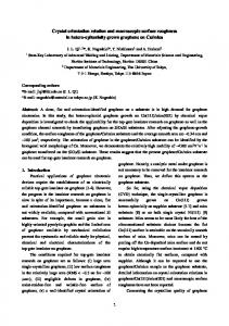
for control parameters that are specified by the optimization algorithm. The optimal controls are those for which the corresponding control parameters lead to a minimum of the objective function. Optimization has been used extensively in the aerodynamic and structural design of aircraft.12,13 These techniques are also well developed for the design of automotive structural components. Optimization techniques are finding increasing applications in chemical processing. For example, Biegler and co-workers14,15 as well as Barton and co-workers16 have developed algorithms for optimizing batch-type industrial chemical processes. Another recent work by Petzold and Zhu17 uses an optimization approach for the reduction of large kinetics mechanisms of chemical processes. The present work discusses the control of chemically reacting flow fields. As a specific example, we demonstrate the optimal control technique on a chemically reacting stagnation flow CVD reactor. The Stagnation Flow Reactor Model Axisymmetric stagnation flow reactors are used extensively in the processing of thin film materials. This reactor configuration consists of an inlet manifold that is placed parallel to and a short distance away from a substrate on which the thin film is deposited. Gases that carry the precursors for film growth enter the reactor through the inlet and impinge normally onto the substrate. Momentum, thermal, and chemical boundary layers develop in the region between the inlet and the substrate. The stagnation flow reactor has several important advantages. Primarily, a proper reactor design assures that the stagnation flowfield within the reaction chamber leads to spatially uniform chemical fluxes at the deposition surface for a wide range of processing conditions.18 A spatially uniform film thickness is, therefore, realized regardless of the chemical properties of the flow. In this way, controls can be implemented to alter the growth conditions while retaining the necessary film uniformity. Figure 1 shows an example of a Navier-Stokes flow solution of the chemically reacting flow field in a stagnation flow reactor. The flat boundary layer indicates that a stagnation flow similarity is realized over the wafer and that edge effects are small. In addition to the physical benefits in CVD, an important advantage of the stagnation flow reactor is that the flowfield can be described mathematically by spatially one-dimensional governing equations (the stagnation flow similarity equations) that are a reduced form of the Navier-Stokes equations.9,20 This mathematical reduction owes to a self-similar nature of the flow where flow variables, either in their primitive form or in a form that is scaled with the radial distance from the centerline, are completely independent of the radius and depend only on the axial coordinate between the inlet and the substrate planes. The reduced dimensionality in the mathematical description of the flowfield greatly facilitates the solution and analysis of the flow and chemical behavior of the gas-phase region between the reactor inlet and the substrate.
Radial momentum r
∂V dV d dV 1 ru 1 m 1 rV 2 1 L r 5 0 ∂t dz dz dz
[3]
Thermal energy rcp
dT d dT ∂T l 1 rucp 2 dz dz dz ∂t K
1
∑ rY U c k
k pk
k =1
dT 1 hk Wk v˙ k 5 0 [4] dz
Species continuity r
∂Yk dY d 1 ru k 1 ( rYk U k ) 2 Wk v˙ k 5 0 ∂t dz dz (k 5 1, . . . , Kg) [5]
Equation of state Kg
ptot 5 rRT
∑ k =1
Yk Wk
[6]
In these equations, the independent variables are the time t and the axial coordinate z. The dependent variables are the excess pressure
Governing equations.—The axisymmetric, stagnation flow similarity equations used in this study are developed in Raja et al.7 These equations incorporate dynamic effects in the stagnation flow field through transient terms and are cast in a compressible form that results in a set of partial-differential algebraic equations. The equations are summarized below. Continuity ∂r d ( ru) r ∂p r ∂T 1 1 2 rV 5 2 ∂t dz ptot ∂t T ∂t Kg
2 pW
∑
k 51
d ( ru) 1 ∂Yk 1 1 2 rV 5 0 [1] Wk ∂t dz
Axial momentum r
∂u ∂u ∂p 1 ru 1 50 ∂t ∂z ∂z
[2]
Figure 1. Results of a Navier-Stokes simulation, showing in gray scales the concentration of the yttrium precursor, Y(thd)3 in a stagnation-flow reactor. The metallorganic precursors enter a heated plenum and mixing chamber at the top of the reactor. A stagnation-flow region is established between a showerhead manifold and a heated wafer surface. Inert, relatively cool purge gases flow downward along the reactor walls. The exhaust gases are pumped out the bottom of the reactor chamber. As evidenced by the radial independence of the concentration field, the ideal stagnation flow is realized over most of the wafer surface.
2720
Journal of The Electrochemical Society, 147 (7) 2718-2726 (2000) S0013-4651(99)10-034-X CCC: $7.00 © The Electrochemical Society, Inc.
p, the axial velocity u, the scaled radial velocity V 5 v/r (v is the radial velocity and r is the radius), the temperature T, and the species mass fractions Yk. The excess pressure is related to the total system pressure ptot using ptot 5 pref 1 p, where pref is a reference pressure that is a specified constant. The mass density r is determined from the equation of state. The pressure gradient term in the radial momentum equation Lr 5 (1/r)(dp/dr) is an eigenvalue that must be determined in the course of the solution. The gas properties cp, l, and m are the constant pressure specific heat, the thermal conductivity, and the viscosity, respectively. The quantities hk and Wk are the species enthalpy and the species molar masses, respectively. The index Kg denotes the total number of gas-phase species. The diffusion velocity of the kth species in the axial direction, Uk 5
1 Xk W
K
∑
Wj Dkj
j?k
∂X j dz
2
DkT 1 ∂T rYk T ∂z
[7]
has an ordinary multicomponent contribution and a thermal diffusive contribution. Here, Dkj is the matrix of ordinary multicomponent diffusion coefficients, and DTk are the thermal diffusion coefficients. The boundary conditions are specified at the inlet manifold as u 5 uin(t), V 5 v/r 5 0, T 5 Tin(t), and Yk 5 Yk,in(t). In the example problems discussed below, the controls are imposed on the species inlet mass fractions and on the inlet axial velocity. At the deposition surface, the boundary conditions include T 5 Tsur(t) and V 5 0. The gas-phase mass fractions at the surface involve the surface chemistry. The surface states are determined from dZ k s˙ 5 k G dt
( k 5 1, . . . , Ks )
[8]
where Zk are the surface site fractions, s?k are the molar production rates of surface species by heterogeneous reaction, and G is the molar density of potentially available surface sites. The index Ks denotes the total number of surface species. The gas-surface coupling is established through the mass-flux balance at the surface rYk(ust 1 Vk) 5 s?kWk
(k 5 1, . . . , Kg)
[9]
where ust is the Stefan velocity. The system of partial differential equations is discretized by a method-of-lines algorithm, wherein the spatial derivatives are approximated using a finite-volume discretization. In the semidiscrete form, the equations become a system of index-two DAEs. The algebraic contributions come from the pressure-curvature eigenvalue Lr, and the discretized continuity equation at the last spatial node adjacent to the inlet manifold. With some manipulation, the equations can be reduced to an index-one system, which is solvable by DAE software such as DASSL or DASPK.21 The gas-phase chemical reaction terms and the gas thermodynamic properties are evaluated using the CHEMKIN package.22 The gas species transport properties are evaluated using the CHEMKIN transport package23 and the surface chemical reactions terms are evaluated using the SURFACECHEMKIN package.24 Chemical reaction mechanism.—Two example problems are considered in this study. The first one involves the deposition of a multicomponent yttrium-barium-copper oxide (YBa2Cu3O7 or simply YBCO) film and the second involves deposition of a single component copper film. b-diketonate metalorganic precursors of the tetramethylheptane dionate (thd) type are assumed as the source of the metal atoms in the films. Table I shows the gas-phase and surface chemical reaction mechanism used in the present study. The gasphase reactions (indicated by the symbol G) account for decomposition of the precursors through oxidative as well as unimolecular routes to form metal atoms. The metal atoms are subsequently oxidized through fast reactions in an oxygen environment. The mechanism postulates that metal atoms and/or metal oxide molecules are the “growth species” and the surface reactions (indicated by S) allow for their incorporation into the bulk film. Only metal oxide incorpo-
Table I. Gas phase and surface reaction mechanism for decomposition of metallorganic precursor molecules and the incorporation of metals into bulk film. Aa
Ea a
02.2 3 1090 4.08 3 1016 2.39 3 1017 1.69 3 1022 6.03 3 1090 fast fast fast 1.0b 1.0b 1.0b
34.30 30.30 52.15 41.10 27.06
Reaction G1 G2 G3 G4 G5 G6 G7 G8 S1 S2 S3
Y(thd)3 r Y 1 p Y(thd)3 1 O2 r Y 1 p Ba(thd)2 r Ba 1 p Ba(thd)2 1 O2 r Ba 1 p Cu(thd)2 r Cu 1 p Y 1 1/2 O2 r YO Ba 1 1/2 O2 r BaO Cu 1 1/2 O2 r CuO YO r YO(d) BaO r BaO(d) CuO r CuO(d)
parameters for the rate constants written in the form: k 5 A exp(2Ea/RT). The units of A are given in terms of moles, cubic centimeters, and seconds. Ea is in kcal/mol. p indicates other reaction products. b Sticking coefficient. A value of 1.0 is simply assumed for this example.
a Arrhenius
ration into the bulk film is shown in Table I; incorporation of metal atoms is assumed to follow the same route. For the present study the surface sticking coefficients for the metal/metal oxides are simply assumed to be one. The intact precursors are assumed to have a negligible sticking coefficient on the surface and do not directly lead to formation of film. The gas-phase reaction rate coefficients are based on experimental data available in the literature.25-27 Dynamic Optimization Algorithm The dynamic optimization algorithm is discussed in detail in Ref. 8, 9, and 10. We review the algorithm here, with a few observations that specifically relate to the chemically reacting stagnation flow optimization problem. The physical problem (discretized form of Eq. 1-5 and Eq. 8 along with boundary conditions) can be represented as a differential-algebraic equation (DAE) system F[t, x, x9, pc, uc(t)] 5 0
x(t0) 5 x0
[10]
where x is a vector of the DAE state variables and the DAE is at most index one.7,21,28 The prime denotes time differentiation. The initial conditions x0 are chosen so that they are consistent (i.e., the algebraic constraints of the DAE are satisfied at time t0). The time-invariant control parameters pc and the time-dependent vector-valued control function uc(t) must be determined such that the objective function F(t f ) 5
∫
tf
t0
c[t, x(t ), p c , u c (t )]dt
[11]
is minimized and some additional inequality constraints G[t, x(t), pc, uc(t)] $ 0
[12]
is are satisfied. The optimal solution for the control function u *(t) c assumed to be continuous. In this application the DAE system is large, i.e., roughly 500 state variables. Thus, the dimension nx of x is large. The dimension of the control parameters and of the number of control functions u c(t) is much smaller. Nevertheless, the optimal control problem is infinite dimensional (since the control functions uc(t) are continuous in time). A control parameterization approach is used to convert the infinite-dimensional optimal control problem to a finite-dimensional one by representing uc(t) in a low-dimensional vector space. For this, piecewise polynomials are constructed within a number of control subintervals [tj, tj11] (j 5 0, . . . , Ntu 2 1, where Ntu is the total number of control subintervals) that divide the total time domain [t0, tf]. The coefficients of the polynomials constitute a finite number of optimization variables. With the control parameter-
Journal of The Electrochemical Society, 147 (7) 2718-2726 (2000)
2721
S0013-4651(99)10-034-X CCC: $7.00 © The Electrochemical Society, Inc.
ization approach we can assume that a vector p contains both the time-invariant control parameters pc and the polynomial coefficients (we let np denote the combined number of these values) and discard the control function uc(t) in the remainder of this paper. Hence, we consider the following dynamic optimization problem minimize subject to
F(t f ) 5
∫
tf
t0
c (t, x(t ), p)dt
F(t, x, x9, p) 5 0
x(t0) 5 x0
g(t, x(t), p) $ 0
[13a] [13b] [13c]
where the optimization constraint Eq. 13b is the problem DAE itself (i.e., the physics must be satisfied) and Eq. 13c is the additional constraint. A number of methods can be used to solve the optimization problem of Eq. 13 by representing the optimal control problem as a nonlinear programming (NLP) program given as minimize
f (pn)
[14a]
subject to
pn l b # F(p n ) # u b Gpn
[14b]
where pn is the vector of optimization variable of the NLP, f(pn) is a scalar-valued NLP objective function and the constraints could include lower (lb) and upper (ub) bounds on the optimization variables pn, vector-valued nonlinear functions F(pn), and a vector-valued linear function represented in the matrix vector product form Gpn. A finite difference or collocation method discretizes the DAEs, Eq. 13b, on a time grid over the interval [t0, tf] with all the discretized DAE solutions x at the time grid points along with the control parameters p as the unknown NLP optimization variables pn. The constraints (Eq. 14b) of the NLP include the finite difference representation of the DAE over the time grid as well as the other constraints (Eq. 13c). The objective function of the NLP, Eq. 14a, is derived from the finite difference representation of Eq. 13a. Although this method is robust and stable, it requires the solution of an optimization problem which can be enormous for a large-scale DAE system, and it does not allow for the use of time-adaptive DAE software. Shooting-type methods offer an alternative to collocation methods. In the single shooting method, which is the technique used for the example problems discussed in this paper, the NLP problem size is considerably smaller with the vector of NLP optimization variables pn including only the optimization parameters p from the optimal control problem, Eq. 13. For some special cases where constraints are imposed on the states of the DAEs at the final time tf and/or if the initial states x0 of the DAE are to be optimized, then the vector pn could include p as well as the DAE states at the initial and/or final time. In any case, the size of the NLP problem does not exceed np 1 2nx. Constraining the piecewise polynomial control functions to be continuous as well as differentiable over the control subinterval interfaces provides the set of linear constraints Gpn for the NLP. The single shooting approach proceeds by solving the DAEs, Eq. 13b, over the interval [t0, tf] using adaptive DAE software (here, we use DASPK.21 The DAE system is augmented by an additional variable y and equation y9 5 c[t, x(t), p]
[15]
so that F(tf) 5 y(tf). Hence, the objective function of the NLP is simply given by f(pn) 5 y(tf). The NLP is solved using SNOPT,11 which implements an iterative SQP algorithm (see Ref. 30). The SQP method satisfies the linear constraints Gpn through all its iterations and hence guarantees that the control functions uc(t) are continuous and differentiable thoughout [t0, tf]. This continuity and differentiability property is important in enabling the DAE solution using DASPK over the time
Figure 2. Illustration of the salient features of single-shooting, optimal control algorithm.
domain. The SQP methods requires the derivative vector (∂f /∂pn) and the Jacobian matrix of the nonlinear constraints (∂F/∂pn). The derivative vector and the Jacobian matrix are computed using a DAE sensitivity algorithm that is incorporated within the DASPK software.31 Also, the sensitivity equations to be solved by DASPK are generated via the automatic differentiation software ADIFOR.32 The basic algorithms and software for the optimal control of dynamical systems are described in detail in Ref. 8 and 10. The single shooting algorithm determines the optimal solution through successive optimization iterations. The process in each optimization iteration is shown schematically in Fig. 2. At each iteration, intermediate values for the optimization variables pn, that include p as a subset, are used to find the continuous control functions uc(t). Given initial conditions x(t0), the controls are then used to solve the stagnation flow DAE system along with the DAE sensitivity equations in the interval [t0, tf] to determine the objective function and the Jacobian matrices. The SQP algorithm then uses this information to determine new guesses for pn which constitutes the next iteration. The process is repeated until converged solutions are obtained for optimal values of pn. A potential disadvantage of the single-shooting approach are that for some problems the algorithm can become unstable, and may require very good initial guess values for pn. Also, it is difficult to implement any additional constraints in the optimal control problem Eq. 13c within the time interval [t0, tf]. For the CVD problems we have considered, the single-shooting approach is stable and has performed very well. However, a new multiple shooting method that is capable of alleviating many of the disadvantages of the single-shooting method has also been developed and holds considerable promise for more general model DAE systems.8,9 Example Problems Stoichiometry control in thin films.—The first example problem considers thin-film polycrystalline high-temperature superconductors of YBa2Cu3O72d for which metallorganic CVD is a standard deposition technique.33-35 Three beta-diketonate metallorganic precursors, Y(thd)3, Ba(thd)2, and Cu(thd)2 carry the metals into the reactor and are dilute in O2 and N2. A wafer surface temperature variation is imposed which constitutes the transient operation. As mentioned in the introduction, such a transient process might be designed to promote film nucleation at one temperature, then transition to another temperature that is preferable for mature film growth. Throughout growth, it is critical to maintain precise ratios of the metal-atom fluxes to the substrate so that the film preserves the correct stoichiometry. If the metal incorporation is permitted to vary too much, either a nonsuperconducting material will grow or phase-segregated nonsuperconducting oxides will appear. Either alternative is unacceptable. Thus, as the surface temperature changes during the process transient, the precursor flow rate at the reactor inlet must be varied to compensate for the temperature dependent effects, in the flow field and the chemistry, and to maintain the correct film composition. Planning these trajectories is the goal of this example problem.
2722
Journal of The Electrochemical Society, 147 (7) 2718-2726 (2000) S0013-4651(99)10-034-X CCC: $7.00 © The Electrochemical Society, Inc.
The metal flux variations at the surface are a consequence of gasphase transport and chemistry effects. As the surface temperature rises, the homogeneous reaction rates in the gas-phase boundary layer increase, accelerating the decomposition of the precursors. Each precursor decomposes differently owing to differences in the activation energies of the various gas-phase chemical reactions. Also, variations in the gas-phase temperature gradients alter the molecular diffusion of species, especially by thermal diffusion for the heavy precursor compounds. Finally, the surface reaction rates depend on the surface temperature. Thus, as the temperature varies, the net gas-phase fluxes of the metal-containing compounds to the surface can vary greatly and nonlinearly. Figure 3 shows gas-phase species profiles for typical YBCO reactor operating conditions at two different substrate temperatures, 900 and 1100 K. The reactor operating conditions are as follows: the reactor pressure is 10 Torr, with a net inlet flow velocity of 200 cm/s and inlet temperature of 500 K. The separation distance between the reactor inlet and the substrate is 3.81 cm. The metal precursors at the inlet are very dilute in a O2/N2 (40/60 by volume) carrier gas. For the results presented in Fig. 3 all three precursors have an equal inlet mole fraction of 1 3 1025. A chemical boundary layer develops above the hot substrate and has a thickness of about 1.5 cm. Within the chemical boundary layer, the metallorganic precursors decompose to form metal oxides that stick to the substrate and are incorporated into the film. The net reaction rates for precursor decomposition vary significantly for the three precursors and depend strongly on the substrate temperature. For both the low and the high temperatures the barium precursor is almost entirely decomposed, thus leading to a high deposition rate of barium oxide molecules on the substrate. The yttrium decomposition rate is relatively low at the lower substrate temperature and is therefore only partially decomposed in the boundary layer with a corresponding low deposition rate of yttrium oxide molecules. At the higher temperature, the yttrium decomposition rate increases significantly with a correspondingly higher deposition rate of yttrium oxide on the substrate. Decomposition rates for the copper precursors have values that are intermediate between those of barium and yttrium. Clearly, the deposition rates of the growth species (metal oxides) depend strongly and nonlinearly on the substrate temperature. Also, sharp gradients and near zero mole fractions of the metal oxides close to the substrate indicate that the growth species deposition rates are limited by the transport in the boundary layer. The film stoichiometry control problem proceeds by assuming that the CVD reactor initially operates under steady-state conditions at a substrate temperature Tsub of 900 K. The initial inlet precursor mole
fractions are chosen such that a 1:2:3 ratio of Y:Ba:Cu metal fluxes deposit onto the surface. For the nominal operating conditions corresponding to results in Fig. 3 with Tsub 5 900 K, the inlet mole fraction of Ba(thd)2 is 0.41 3 1025 and of Cu(thd)2 is 0.63 3 1025 for a Y(thd)3 inlet mole fraction of 1 3 1025. These inlet conditions result in stoichiometric films at Tsub 5 900 K but produce highly off-stoichiometric films for other temperatures. When a transient is imposed during reactor operation by changing the substrate temperature, two of the three inlet precursor mole fractions must be changed along some unknown trajectories in time so as to obtain stoichiometric film deposition throughout the duration of the transient. The optimal control algorithm determines these inlet mole fraction trajectories. In this problem, we have chosen (somewhat arbitrarily) to hold the yttrium precursor inlet mole fraction fixed in time while the barium and copper precursor mole fractions are controlled. The substrate temperature is varied from 900 to 1100 K in a 1 min transient along a cosine trajectory given by 0 Tsub (t ) 5 Tsub 1
DT 2
t cos p 2 1 1 1 t f
0 is the initial temperature (900 K), DT is the temperature where T sub difference between the initial and final state (200 K), tf is the final time (60 s) and the initial time is assumed as t 5 0. The time interval from 0 to 60 s is subdivided into 10 equal control intervals and a second order (quadratic) polynomial representation of the controls is assumed in each interval. The quadratic approximation is the lowest order polynomial on which the linear continuity and differentiability constraints can be imposed while still being able to represent a sufficiently complicated control over the time domain. Since the precursor concentration in the carrier gas is very dilute and the decomposition chemistries of each the precursors are independent of each other, the size of the computational problem can be reduced by considering just two of the precursors at a time. First, the yttrium and barium precursor combination is considered, in order to determine the optimal trajectory of the barium inlet mole fraction. Following this, the yttrium and copper precursor combination is considered, in order to determine the trajectory of the copper inlet precursor mole fraction. In both cases, the yttrium inlet mole fraction is held fixed in time. The stagnation flow model uses 30 grid points in the axial direction with grid clustering near the substrate. The DAE problem size for each of the two precursor combinations is 423 states. Accounting for control continuity and differentiability at the control interval interfaces, the optimization problem has 12 independent control parameters (control polynomial coefficients). The cost function for this problem is constructed to penalize off stoichiometric deposition at the substrate at any given time during the transient. A suitable integrand of the cost function Eq. 13a for this problem is
s˙ / n c(t, x (t ), p) 5 1 2 e e s˙ Y
Figure 3. Stagnation flow gas phase species profiles at two different substrate temperatures of 900 and 1100 K.
[16]
2
[17]
where the surface mole fluxes of the metal atoms are given by s?e and ne represents the stoichiometric coefficients of the metal atoms in the film (ne 5 2 for barium and ne 5 3 for copper). The subscript Y represents the yttrium atom while e generically represents the barium and copper atoms. When no control is implemented (the precursor inlet mole fractions are constant throughout the transient) the value of the cost function F(tf) equals 20.6 and 14.5 for the yttrium plus barium and yttrium plus copper cases, respectively. The optimal solutions that are discussed below correspond to cost function values that are less than 1022. It must also be noted that while the above objective function represents a simple measure of the quality of the film, one could certainly design more complex functions. For example, nonsymmetric cost functions that preferentially penalize films which are excess is certain metals compared to films that are deficient in the same metals could be developed. This is certainly an
Journal of The Electrochemical Society, 147 (7) 2718-2726 (2000)
2723
S0013-4651(99)10-034-X CCC: $7.00 © The Electrochemical Society, Inc.
important factor in obtaining good quality YBCO films where barium rich films are not superconducting and hence unacceptable while films that are slightly deficient in barium are acceptable as superconductors. Optimal solutions for film stoichiometry control problem are shown in Fig. 4 along with the imposed substrate temperature trajectory. As we have already seen in Fig. 3, an increase in the substrate temperature results in an increase in the deposition flux of yttrium atoms. Since the barium and copper precursor molecules are decomposed to a relatively higher degree than yttrium at 900 K, the only way to keep the metal deposition ratios at the surface constant is to increase the inlet mole fractions of barium and copper. This is more so for barium, whose precursors molecules are almost entirely decomposed in the boundary layer even at the lower temperature of 900 K. The inlet mole fraction trajectories for barium and copper precursors normalized by their initial inlet mole fractions clearly illustrates this point. The surface deposition ratios of barium to yttrium (Ba/Y) and copper to yttrium (Cu/Y) are shown in Fig. 5. With control, the Ba/Y and Cu/Y ratios remain very close to 2 and 3, respectively, throughout the transient. Without control, i.e., if all three inlet mole fractions were held constant through the transient, the films would be highly deficient in both barium and copper when compared to the proportion of yttrium in the film. The need for stoichiometry control through manipulation of the inlet composition of individual precursors during an imposed transient is readily apparent.
Figure 5. Barium and copper atom to yttrium atom deposition ratios for cases with and without controls.
Precursor utilization and deposition time optimization.—A second example of optimal control of transient CVD processing considers the deposition of a single-component film. Here, the notion of a composite cost function, which represents multiple and disparate objectives, is developed. This example problem is also different from the previous one in that deposition time (DAE problem time) is one of the optimization variables. Moreover, constraints (bounds) are imposed on the control variables. We consider the deposition of copper films in a stagnation flow reactor that operates under the same nominal operating conditions as in the previous example. The gas-phase chemistry involves only the step that results in the decomposition of the copper precursor molecules to produce copper atoms. The step that results in subsequent oxidation of the copper atoms is neglected and the copper atoms themselves are the growth species. The substrate temperature is kept
fixed at 1100 K. The statement of the optimal control problem is as follows: a copper film of a precise thickness is to be deposited, subject to the requirements of maximum precursor utilization (minimum precursor waste) and minimum deposition time. The control variables are the reactor inlet flow rate (inlet velocity) and the mole fraction of the copper precursor at the reactor inlet. An opportunity for optimal control exists in this problem because of the conflicting reactor operational requirements for increasing film deposition rate and minimizing precursor bypass. For a fixed stagnation-flow reactor geometry with a fixed precursor inlet mole fraction, an increase in the reactor inlet velocity causes the precursor bypass to increase and the film deposition rate to either increase or decrease. For a fixed inlet velocity, an increase in the precursor inlet mole fraction causes the film deposition rate to increase. These dependencies can be understood based on the species profiles shown in Fig. 3 and a mathematical simplification of the same shown in Fig. 6. The precursor mole fraction remains a constant value Xpre until it enters the boundary layer where it begins to decompose to produce intermedi-
Figure 4. Imposed substrate temperature trajectory and the normalized inlet mole fraction control trajectories for the barium and copper precursors. The control trajectories are normalized by the inlet mole fractions of 0.43 3 1025 and 0.63 3 1025 for the barium and copper precursors, respectively.
Figure 6. Mathematical representation of the species profiles in a stagnationflow boundary layer with precursors and intermediate species. The intermediate species are assumed to lead to film growth.
2724
Journal of The Electrochemical Society, 147 (7) 2718-2726 (2000) S0013-4651(99)10-034-X CCC: $7.00 © The Electrochemical Society, Inc.
ate film growth species (in this case metal atoms). The intermediate species stick to the film surface, and hence, a peak value in the mole fraction Xint is observed within the boundary layer. The composition boundary layer thickness dbl can be conveniently defined as the distance between the location of this peak and the deposition surface, as shown in Fig. 6. The film deposition rate is proportional to the molar flux of copper atoms to the substrate, which in turn depends on dbl and Xint. The film deposition rate is therefore given as Gfilm , D
X int 2 0 d bl
[18]
where the zero approximates the growth species mole fraction at the substrate for the gas transport limited growth regime. The species diffusion coefficient is given by D. It is well known that the stagnation flow boundary layer thickness dbl scales approximately with the inlet velocity uinl as36,37 d bl ,
1 2 u1/ inl
[19]
For dilute precursor concentrations in the carrier gas, Xint is proportional to the precursor inlet mole fraction Xpre. Also, Xint depends in some nonlinear fashion on the flow residence time tbl and the gasphase precursor decomposition reaction rate coefficient. The flow residence time can be defined as tbl 5 dbl/uinl and hence t bl ,
1 3/ 2 uinl
[20]
In general, Xint decreases with decreasing tbl, due to reduced time available for the decomposition reaction to proceed, and hence for a given precursor decomposition rate coefficient, Xint decreases as uinl increases. Assuming a power-law relationship for the above dependence, Xint has the following dependence on the reactor control variables uinl and Xpre Xint , u2q int Xpre
[21]
where the exponent q is a positive number. Therefore, the film deposition rate depends on the control variables as Gfilm , Du1/22q inl Xpre
[22]
For nominal operating conditions of the copper deposition reactor assumed in this study, q < 1/2 and therefore increasing uinl increases Gfilm and increasing Xpre increases Gfilm. The influence of the controls on the precursor bypass is easily understood by observing that decreasing dbl (by increasing uinl) results in an increasing fraction of the carrier and active gases, that enter the reactor through the inlet, being lost through the reactor exhaust without participating in the deposition process in the boundary layer. Hence, increasing uinl increases precursor bypass. The optimal control problem assumes that steady-state flow conditions are initially established in the reactor with a zero precursor mole fraction at the inlet and an inlet flow velocity of 200 cm/s. The first control variable, i.e., the precursor mole fraction at the inlet Xpre, is increased as the transient begins, to deposit a 5 nm thick copper film. The second control variable, i.e., the inlet velocity uinl, is also modified during the transient. Constraints are imposed on the extent to which the control can be modified. The value of the inlet mole fraction of the precursor is constrained to be less than 5 3 1024 and the inlet velocity is constrained to be between 50 and 400 cm/s, throughout the transient. Also, Xpre is constrained to zero at the final time. An additional differential equation is solved to determine the film height as a function of time. The equation is W n s˙ dh 5 film int int r film dt
[23]
where Wfilm is the film molar mass, rfilm is the film density, s?int is the molar deposition rate of the growth species, and nint is the number of
metal atoms per molecule of the growth species. To achieve a desired film thickness at the end of the deposition time tf, an equality constraint of the form h(tf) 5 hfilm
[24]
is implemented where hfilm is the desired film thickness. Since the total deposition time enters as one of the optimization variables, the DAE integration problem requires a slight modification. In addition to the optimization parameters obtained from the continuous control parameterization, a new optimization variable pt is introduced so that the physical problem time is defined as t 5 tpt,
t [ [0, tf]
[25]
where t [ [0, tref] is the DAE integration time. The quantity pt is an additional variable that is optimized, while the final DAE integration time tref is fixed. The stagnation-flow governing DAEs and the corresponding sensitivity equations are solved on the fixed integration time interval [0, tref] with t as the independent variable. All time derivatives in the governing equations are scaled as d 1 d 5 dt pt dt
[26]
The integrand of the multiobjective cost function is Ainl r inl X preU inl / W c[t, x (t ), p] 5 a 1 bpt Asub hfilm r film /(t ref Wfilm )
[27]
where Ainl and Asub are the reactor inlet and substrate areas, rinl is the density of the gas at the inlet, and W w is the mean molar mass of the gas at the inlet. The first term represents the cost associated with the precursor entering the reactor (i.e., a measure of precursor bypass) and the second term represents cost associated with processing time. The numerator of the first term equals the molar flow rate of the metal precursor molecules entering the reactor at a given time. The denominator of the first term represents a measure of the molar deposition rate of the metal atoms at the film and is used to nondimensionalize the inlet molar flow rate of the metal atoms. Values of the constants a and b are chosen to reflect the relative importance of the precursor utilization as compared to the total deposition time in the optimization problem. The DAE problem has 275 state variables with 30 grid points in the axial direction of the stagnation flow field and the optimization problem has 25 control parameters, including pt. In this problem tref 5 60 s. Constraints are placed on pt so that its value is between 0.7 and 1.6. For the copper film considered here, Wfilm 5 63.54 g/mol, rfilm 5 8.96 g/cm3, and nint 5 1. Optimal solutions are obtained for three combinations of values of a and b. For the case where only the precursor utilization is important, a 5 1 and b 5 0; when only deposition time is important a 5 0 and b 5 1; and when both precursor utilization and deposition time are important a 5 0.5 and b 5 0.5. Optimal values for the precursor inlet mole fraction are shown in Fig. 7 and for the inlet velocity are shown in Fig. 8. When only the precursor utilization is important (a 5 1 and b 5 0) the deposition time is maximized to the extent allowed by the constraints on pt, i.e., pt 5 1.6 (corresponding to tf 5 96 s). The precursor inlet mole fraction Xpre ramps up slowly to reach a peak of about 4 3 1024 at about 50 s, following which the mole fraction ramps down to zero at the final time. During this time, the inlet velocity drops slowly to reach the lower bound of 50 cm/s in about 20 s and remains at this value through most of the transient before slowly increasing in magnitude in the last 15 s. For the case where only deposition time is important (a 5 0 and b 5 1) the deposition time is minimized and the optimal value of pt is at the lower bound, i.e., pt 5 0.7 (corresponding to tf 5 42 s). The optimal control values indicate that both Xpre and Uinl increase rapidly to peak values at about 24 s. The peak value of the precursor inlet mole fraction is about 1.9 3 1024. The peak inlet velocity is about 300 cm/s.
Journal of The Electrochemical Society, 147 (7) 2718-2726 (2000)
2725
S0013-4651(99)10-034-X CCC: $7.00 © The Electrochemical Society, Inc.
Figure 7. Optimal trajectories of the precursor inlet mole fraction. The thin vertical lines indicate the bounds on the deposition time. a 5 1 and b 5 0 corresponds to only the precursor utilization being important; a 5 0 and b 5 1 corresponds to only the deposition time being important; and a 5 0.5 and b 5 0.5 corresponds to both precursor utilization and deposition time being important.
When both precursor utilization and deposition time are important factors in the cost function (a 5 0.5 and b 5 0.5), the optimal deposition time corresponds to pt 5 0.87 (corresponding to tf < 52 s). The precursor inlet mole fraction reaches a peak value of 5 3 1024 (equal to the upper bound) at around 30 s while the inlet velocity drops sharply to reach the lower bound of 50 cm/s before increasing toward the end of the transient. The oscillations seen in the value of Uinl close to its lower bound is one of the deficiencies of the control parameterization approach, since the bound values are enforced only at the control interval interfaces. The polynomial representation of the controls therefore allow for a violation of the bounds at intermediate times, without the optimization constraints themselves being violated. One approach to alleviate this problem would be to include an additional term in the cost function that penalizes high values of the time derivatives of the control, hence damping the oscillatory behavior. Alternatively, one could simply disregard the oscillations while interpreting the solution.
Figure 9. Film thickness as a function of time. See caption of Fig. 7 for explanation of the different a and b combinations.
The film thickness during deposition is shown in Fig. 9. The thickness at the final time of the deposition equals 5 nm for all three cases, thus indicating that the equality constraint on the film thickness is satisfied. Conclusions Time varying chemical vapor deposition processing is an alternative that potentially offers significant advantages over traditional steady processing techniques. Optimal trajectory planning is an important approach to assist development of such processes. The overall strategy is to design path following processes that miminimize a specified cost function. In this work, a transient, stagnation flow model of a CVD reactor is coupled with an optimization algorithm to enable trajectory planning for the reactor controls. The algorithm is demonstrated successfully using two examples problems. The first example demonstrates the need for controlling reactor inlet composition to achieve correct film stoichiometry while the reactor itself is subjected to an imposed wafer-temperature ramp. In the second example, trajectories for reactor inlet velocity and precursor concentration are determined for deposition of copper films of a desired thickness. These trajectories are optimal with regards to multiple and conflicting objectives of maximum precursor utilization and minimum time for film deposition. The method and software are shown to be very general, with potentially wide applications. Acknowledgments This work was supported by NSF and DARPA within the Virtual Integrated Processing program. The Colorado School of Mines assisted in meeting the publication costs of this article.
References
Figure 8. Optimal trajectories of the reactor inlet velocity. The thin vertical lines indicate the bounds on the deposition time. See caption of Fig. 7 for explanation of the different a and b combinations.
1. C. A. Wolden, C. E. Draper, Z. Sitar, and J. T. Prater, J. Mater. Res., 14, 259 (1999). 2. X. Li, P. Sheldon, H. Moutinho, and R. Matson, in Proceedings of the 25th Photovoltaics Specialists Conference, IEEE, pp. 933, Washington, DC (1996). 3. T. S. Cale, M. K. Jain, and G. B. Raupp, J. Electrochem. Soc., 137, 1526 (1990). 4. D. Yang, R. Jonnalagadda, B. R. Rogers, J. T. Hillman, R. F. Foster, and T. S. Cale, Abstract 351, The Electrochemical Society Meeting Abstracts, Vol. 98-2, Boston, MA, Nov 1-6, 1998. 5. A. E. Braun, Semicond. Int., 22, 56 (1999). 6. A. Agarwal, A. T. Fiory, and A-J. L. Grossmann, Semicond. Int., 22, 71 (1999). 7. L. L. Raja, R. J. Kee, and L. R. Petzold, in Twenty Seventh Symposium (International) on Combustion, pp. 2249, The Combustion Institute, Pittsburgh, PA (1998). 8. L. R. Petzold, J. B. Rosen, P. E. Gill, L. O. Jay, and K. Park, in Large Scale Optimization with Applications, Part II: Optimal Design and Control, Vol. 93, p. 271, L. Biegler, T. Coleman, A. Conn, and F. Santosa, Editors, IMA (1997). 9. P. E. Gill, L. O. Jay, M. W. Leonard, L. R. Petzold, and V. Sharma, J. Comp. Appl. Math, To be published (1999). 10. R. Serban, UCSB Technical Report, UCSB-ME-99-1 (1999).
2726
Journal of The Electrochemical Society, 147 (7) 2718-2726 (2000) S0013-4651(99)10-034-X CCC: $7.00 © The Electrochemical Society, Inc.
11. P. E. Gill, W. Murray, and M. A. Saunders, Numerical Analysis Report 97-2, Department of Mathematics, University of California, San Diego, La Jolla, CA (1997). 12. J. Sobieszczanski-Sobieski and R.T. Haftka, Structural Optimization, 14, 1 (1997). 13. R. Celi, J. Aircraft, 36, 176 (1999). 14. L. T. Biegler, J. Process Control, 8, 301 (1998). 15. A. Cervantes and L. T. Biegler, AIChE J., 44, 1038 (1998). 16. P. I. Barton, R. J. Allgor, W. F. Feehery, and S. Galan, Ind. Eng. Chem. Res., 37, 966 (1998). 17. L. R. Petzold and W. Zhu, AIChE J., 45, 869 (1998). 18. C. Houtman, D. B. Graves, and K. F. Jensen, J. Electrochem. Soc., 133, 961 (1986). 19. T. W. Chapman and G. L. Bauer, Appl. Sci. Res., 31, 223 (1975). 20. K. Sheshadri and F. A. Williams, Int. J. Heat Mass Transfer, 21, 251 (1978). 21. K. E. Brenan, S. L. Campbell, and L. R. Petzold, Numerical Solution of InitialValue Problems in Differential-Algebraic Equations, 2nd ed., SIAM Publications, Philadelphia, PA (1995). 22. R. J. Kee, F. M. Rupley, E. Meeks, and J. A. Miller, SAND96-8216, Sandia National Laboratories Report, Albuquerque, NM (1996). 23. R. J. Kee, G. Dixon-Lewis, J. Warnatz, M. E. Coltrin, and J. A. Miller, SAND868246, Sandia National Laboratories Report, Albuquerque, NM (1995). 24. M. E. Coltrin, R. J. Kee, F. M. Rupley, and E. Meeks, SAND96-8217, Sandia National Laboratories Report, Albuquerque, NM (1996).
25. A. Y. Kovalgin, F. Chabert-Rocabois, M. L. Hitchman, S. H. Shamlin, and S. E. Alexandrov, J. Phys. IV, C5, C5-357 (1995). 26. M. L. Hitchman, S. H. Shamlin, G. C. Guglielmo, and F. Chabert-Rocabois, J. Alloys Compd., 251, 297 (1997). 27. A. F. Bykov, P. P Semyannikov, and I.K. Igumenov, J. Therm. Anal., 38, 1477 (1992). 28. U. M. Ascher and L. R. Petzold, Computer Methods for Ordinary Differential Equations and Differential-Algebraic Equations, SIAM Publications, Philadelphia, PA (1998). 29. U. M. Ascher, R. M. Mattheij, and R. D. Russell, Numerical Solution of Boundary Value Problems for Ordinary Differential Equations, SIAM Publications, Philadelphia, PA (1995). 30. P. E. Gill, W. Murray, and M. H. Wright, Practical Optimization, Academic Press, New York (1981). 31. T. Maly and L. R. Petzold, Appl. Num. Math., 20, 57 (1996). 32. C. Bischof, A. Carle, G. Corliss, A. Griewank, and P. Hovland, Scientific Programming, 1, 11 (1992). 33. I. M. Watson, Chem. Vap. Deposition, 3, 9 (1997). 34. K.-H. Dahmen and T. Gerfin, Prog. Cryst. Growth and Charact., 27, 117 (1993). 35. M. Leskela, H. Molsa, and L. Niinisto, Supercond. Sci. Technol., 6, 627 (1993). 36. F. M. White, Viscous Fluid Flow, 2nd ed., McGraw-Hill Inc., New York (1991). 37. D. S. Dandy and J. Yun, J. Mater. Res., 12, 1112 (1997).