Computational approaches for RNA energy ... - Semantic Scholar

Computational approaches for RNA energy parameter estimation by Mirela S¸tefania Andronescu

M.Sc., The University of British Columbia, 2003 B.Sc., Bucharest Academy of Economic Studies, 1999

A THESIS SUBMITTED IN PARTIAL FULFILMENT OF THE REQUIREMENTS FOR THE DEGREE OF Doctor of Philosophy in The Faculty of Graduate Studies (Computer Science)

The University Of British Columbia (Vancouver) November, 2008 c Mirela S¸tefania Andronescu 2008

ii

Abstract RNA molecules play important roles, including catalysis of chemical reactions and control of gene expression, and their functions largely depend on their folded structures. Since determining these structures by biochemical means is expensive, there is increased demand for computational predictions of RNA structures. One computational approach is to find the secondary structure (a set of base pairs) that minimizes a free energy function for a given RNA conformation. The forces driving RNA folding can be approximated by means of a free energy model, which associates a free energy parameter to a distinct considered feature. The main goal of this thesis is to develop state-of-the-art computational approaches that can significantly increase the accuracy (i.e., maximize the number of correctly predicted base pairs) of RNA secondary structure prediction methods, by improving and refining the parameters of the underlying RNA free energy model. We propose two general approaches to estimate RNA free energy parameters. The Constraint Generation (CG) approach is based on iteratively generating constraints that enforce known structures to have energies lower than other structures for the same molecule. The Boltzmann Likelihood (BL) approach infers a set of RNA free energy parameters which maximize the conditional likelihood of a set of known RNA structures. We discuss several variants and extensions of these two approaches, including a linear Gaussian Bayesian network that defines relationships between features. Overall, BL gives slightly better results than CG, but it is over ten times more expensive to run. In addition, CG requires software that is much simpler to implement. We obtain significant improvements in the accuracy of RNA minimum free energy secondary structure prediction with and without pseudoknots (regions of non-nested base pairs), when measured on large sets of RNA molecules with known structures. For the Turner model, which has been the gold-standard model without pseudoknots for more than a decade, the average prediction accuracy of our new parameters increases from 60% to 71%. For two models with pseudoknots, we obtain an increase of 9% and 6%, respectively. To the best of our knowledge, our parameters are currently state-of-the-art for the three considered models.

iii

Contents Abstract . . . . . . . . . . . . . . . . . . . . . . . . . . . . . . . . . . . .

ii

Contents . . . . . . . . . . . . . . . . . . . . . . . . . . . . . . . . . . . .

iii

List of Tables . . . . . . . . . . . . . . . . . . . . . . . . . . . . . . . . .

vi

List of Figures . . . . . . . . . . . . . . . . . . . . . . . . . . . . . . . . viii Glossary . . . . . . . . . . . . . . . . . . . . . . . . . . . . . . . . . . . .

x

Acknowledgements . . . . . . . . . . . . . . . . . . . . . . . . . . . . . xiii Dedication . . . . . . . . . . . . . . . . . . . . . . . . . . . . . . . . . . . xiv 1 Introduction . . . . . . . . . . . . . . . . . . . . . . . . . 1.1 RNA secondary structures and prediction . . . . . . . 1.2 RNA thermodynamics and free energy models . . . . . 1.3 The RNA parameter estimation problem and accuracy 1.4 Contributions . . . . . . . . . . . . . . . . . . . . . . . 1.5 Thesis outline . . . . . . . . . . . . . . . . . . . . . . .

. . . . . . . . . . . . . . . . . . measures . . . . . . . . . . . .

2 Background and related work . . . . . . . . . . . . . . . . . . 2.1 RNA secondary structure prediction algorithms . . . . . . . . 2.1.1 Free energy minimization algorithms . . . . . . . . . . 2.1.2 Partition function algorithms . . . . . . . . . . . . . . 2.1.3 Secondary structure prediction including pseudoknots 2.1.4 Comparative structure prediction . . . . . . . . . . . . 2.2 RNA energy models . . . . . . . . . . . . . . . . . . . . . . . 2.2.1 The Turner model . . . . . . . . . . . . . . . . . . . . 2.2.2 Other RNA energy models . . . . . . . . . . . . . . . 2.3 Computational methods for RNA parameter estimation . . . 2.4 Related parameter estimation algorithms . . . . . . . . . . . 2.5 Summary . . . . . . . . . . . . . . . . . . . . . . . . . . . . . 3 Data collection . . . . . . . . . . . . . 3.1 RNA STRAND: A new database of 3.1.1 Content and construction . 3.1.2 Utility . . . . . . . . . . . .

1 2 6 11 13 15

. . . . . . . . . . . .

. . . . . . . . . . . .

16 16 16 18 19 20 21 21 25 27 28 29

. . . . . . . . . . . . . . . . RNA secondary structures . . . . . . . . . . . . . . . . . . . . . . . . . . . . . . . .

. . . .

31 33 34 38

iv

Contents 3.1.3 Processing the RNA STRAND data . . . . . . . . RNA THERMO: A new database of optical melting data 3.2.1 Analysis of RNA THERMO . . . . . . . . . . . . . Summary . . . . . . . . . . . . . . . . . . . . . . . . . . .

. . . .

. . . .

. . . .

. . . .

41 45 45 53

4 RNA parameter estimation algorithms . . . . . . . . . . 4.1 The Constraint Generation (CG) approach . . . . . . . . 4.1.1 The basic CG algorithm . . . . . . . . . . . . . . . 4.1.2 NOM-CG: NO Max-margin CG . . . . . . . . . . . 4.1.3 DIM-CG: DIrect Max-margin CG . . . . . . . . . 4.1.4 LAM-CG: Loss-Augmented Max-margin CG . . . 4.1.5 Implementation . . . . . . . . . . . . . . . . . . . . 4.2 The Boltzmann Likelihood (BL) approach . . . . . . . . . 4.2.1 The BL algorithm . . . . . . . . . . . . . . . . . . 4.2.2 Relationship between BL and DIM-CG . . . . . . 4.2.3 Implementation . . . . . . . . . . . . . . . . . . . . 4.3 The Bayesian Boltzmann Likelihood (BayesBL) approach 4.3.1 Bayesian prediction . . . . . . . . . . . . . . . . . 4.3.2 Sampling from the posterior distribution . . . . . . 4.3.3 Implementation . . . . . . . . . . . . . . . . . . . . 4.4 Summary . . . . . . . . . . . . . . . . . . . . . . . . . . .

. . . . . . . . . . . . . . . .

. . . . . . . . . . . . . . . .

. . . . . . . . . . . . . . . .

. . . . . . . . . . . . . . . .

54 54 54 58 60 62 63 64 64 67 68 69 70 71 72 72

5 Parameter estimation for the Turner99 model 5.1 Model description . . . . . . . . . . . . . . . . . 5.2 Data sets . . . . . . . . . . . . . . . . . . . . . 5.3 Algorithm configuration for CG . . . . . . . . . 5.4 Algorithm configuration for BL . . . . . . . . . 5.5 Sensitivity to the training structural set . . . . 5.6 Results of the BayesBL approach . . . . . . . . 5.7 Comparative accuracy analysis . . . . . . . . . 5.8 Runtime analysis . . . . . . . . . . . . . . . . . 5.9 Summary . . . . . . . . . . . . . . . . . . . . .

3.2 3.3

. . . . . . . . . .

. . . . . . . . . .

. . . . . . . . . .

. . . . . . . . . .

. . . . . . . . . .

. . . . . . . . . .

. . . . . . . . . .

. . . . . . . . . .

. . . . . . . . . .

. . . . . . . . . .

74 74 76 77 80 82 84 87 96 99

6 Model selection and feature relationships . . . . . . . . 6.1 Linear Gaussian Bayesian network . . . . . . . . . . . . 6.2 Variations of the Turner model and feature relationships 6.3 Results . . . . . . . . . . . . . . . . . . . . . . . . . . . . 6.3.1 Model selection results . . . . . . . . . . . . . . . 6.3.2 Accuracy when using feature relationships . . . . 6.3.3 Comparative accuracy analysis . . . . . . . . . . 6.3.4 Runtime analysis . . . . . . . . . . . . . . . . . . 6.4 Summary . . . . . . . . . . . . . . . . . . . . . . . . . .

. . . . . . . . .

. . . . . . . . .

. . . . . . . . .

. . . . . . . . .

. . . . . . . . .

101 102 104 112 112 118 118 123 124

v

Contents 7 Parameter estimation for pseudoknotted models . . . . . . . . 7.1 Pseudoknotted models . . . . . . . . . . . . . . . . . . . . . . . . 7.1.1 The Dirks & Pierce (DP) model . . . . . . . . . . . . . . 7.1.2 The Cao & Chen (CC) model . . . . . . . . . . . . . . . . 7.2 Prediction and parameter estimation algorithms . . . . . . . . . 7.2.1 Prediction algorithm: HotKnots . . . . . . . . . . . . . . 7.2.2 Parameter estimation algorithm: extension of CG . . . . 7.3 Data sets . . . . . . . . . . . . . . . . . . . . . . . . . . . . . . . 7.3.1 Structural data . . . . . . . . . . . . . . . . . . . . . . . . 7.3.2 Thermodynamic data . . . . . . . . . . . . . . . . . . . . 7.4 Results . . . . . . . . . . . . . . . . . . . . . . . . . . . . . . . . . 7.4.1 Accuracy of the previous parameters . . . . . . . . . . . . 7.4.2 CG algorithm configuration for the pseudoknotted models 7.4.3 Comparative accuracy analysis . . . . . . . . . . . . . . . 7.4.4 Runtime analysis . . . . . . . . . . . . . . . . . . . . . . . 7.5 Summary . . . . . . . . . . . . . . . . . . . . . . . . . . . . . . .

125 125 126 127 129 129 129 130 130 132 133 133 136 138 141 143

8 Conclusions and directions for future work 8.1 Data sets and accuracy measures . . . . . . 8.2 Parameter estimation algorithms . . . . . . 8.3 RNA free energy models . . . . . . . . . . . 8.4 RNA secondary structure prediction . . . . 8.5 Summary . . . . . . . . . . . . . . . . . . .

146 146 149 153 154 157

. . . . . .

. . . . . .

. . . . . .

. . . . . .

. . . . . .

. . . . . .

. . . . . .

. . . . . .

. . . . . .

. . . . . .

. . . . . .

. . . . . .

Bibliography . . . . . . . . . . . . . . . . . . . . . . . . . . . . . . . . . 158 A Loss-augmented RNA secondary structure prediction . . . . . 173 B Computation of partition function and gradient, no dangles B.1 Partition function . . . . . . . . . . . . . . . . . . . . . . . . . . B.2 Base pair probabilities . . . . . . . . . . . . . . . . . . . . . . . B.3 Partition function gradient . . . . . . . . . . . . . . . . . . . .

. . . .

178 179 180 181

C Computation of partition function and gradient, with dangles C.1 Partition function . . . . . . . . . . . . . . . . . . . . . . . . . . . C.2 Base pair probabilities . . . . . . . . . . . . . . . . . . . . . . . . C.3 Partition function gradient . . . . . . . . . . . . . . . . . . . . .

184 185 189 191

D Parameter sets for the Turner99 features . . . . . . . . . . . . . 198 E Collaborations . . . . . . . . . . . . . . . . . . . . . . . . . . . . . . 203

vi

List of Tables 3.1 3.2 3.3 3.4 3.5 3.6 4.1 5.1 5.2 5.3 5.4 5.5 5.6 5.7 5.8 6.1 6.2 6.3 6.4 6.5 6.6 7.1

The main RNA types included in RNA STRAND v2.0 . . . . . . Statistics on the complexity of pseudoknots in RNA STRAND v2.0 The main RNA types included in RNA STRAND, and in our structural set. . . . . . . . . . . . . . . . . . . . . . . . . . . . . . Summary of RNA THERMO . . . . . . . . . . . . . . . . . . . . Regression analysis on T-Full . . . . . . . . . . . . . . . . . . . . Regression analysis on T-Full, when the precision of the Xia et al. experiments is increased. . . . . . . . . . . . . . . . . . . . . . Overview of our three approaches to solving the RNA parameter estimation problem. . . . . . . . . . . . . . . . . . . . . . . . . . Summary of the features in the basic Turner99 model . . . . . . Structural data sets used for training, validation and testing for the Turner99 model . . . . . . . . . . . . . . . . . . . . . . . . . Hold-out validation of the CG input arguments for the Turner99 model . . . . . . . . . . . . . . . . . . . . . . . . . . . . . . . . . Hold-out validation of the BL input arguments for the Turner99noD model . . . . . . . . . . . . . . . . . . . . . . . . . . . . . . Cross-validation of BL, DIM-CG and LAM-CG . . . . . . . . . . Parameter estimation when using different structural training sets Results of BL and BayesBL when training on 1/64 S-Full-Train . Accuracy comparison of various parameter training methods. . .

36 39 42 46 47 49 73 75 76 79 80 82 83 85 88

Summary of the features for the basic Turner99, Parsimonious and Lavish RNA models. . . . . . . . . . . . . . . . . . . . . . . 111 Summary of parameter estimation results for various combined parsimonious and lavish models. . . . . . . . . . . . . . . . . . . 113 Summary of parameter estimation results for various combined basic Turner99, parsimonious and lavish models . . . . . . . . . . 114 BL and BL-FR results on several training sets, from small to large117 Results when including feature relationships. . . . . . . . . . . . 120 Runtime analysis of BL and BL-FR on various models . . . . . . 123 Summary of The Dirks & Pierce and Cao & Chen pseudoknotted models . . . . . . . . . . . . . . . . . . . . . . . . . . . . . . . . . 127

List of Tables 7.2 7.3 7.4 7.5 7.6 7.7

Features for pseudoknots used in the Dirks & Pierce model in addition to the Turner features . . . . . . . . . . . . . . . . . . . Structural data used for pseudoknotted parameter estimation . . Structural and thermodynamic data sets used for training and testing for pseudoknotted parameter estimation . . . . . . . . . . Summary of prediction accuracy for three models with and without pseudoknots, when using various model parameters . . . . . CG algorithm configuration for the Dirks & Pierce model . . . . CG algorithm configuration for the Cao & Chen model. . . . . .

D.1 The features and various parameter sets for the Turner99 model

vii

128 130 132 135 136 137 202

viii

List of Figures 1.1 1.2 2.1 3.1 3.2 3.3

3.4 3.5 4.1 4.2 4.3 4.4 5.1 5.2 5.3 5.4 5.5 5.6

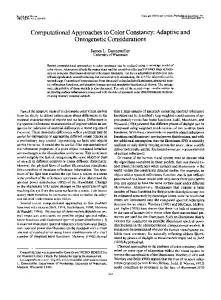
Example of an RNA secondary structure. . . . . . . . . . . . . . Known and predicted structures for the RNA subunit of the signal recognition particle molecule of Desulfovibrio vulgaris. . . . . . .

10

Secondary structure of an arbitrary RNA sequence, showing the main structural motifs. . . . . . . . . . . . . . . . . . . . . . . . .

22

Schematic representation of the data sets used for the RNA parameter learning problem. . . . . . . . . . . . . . . . . . . . . . . Construction of RNA STRAND, from the data collection to the data presentation via dynamic web pages . . . . . . . . . . . . . Histogram of non-canonical base pairs in the 729 non-redundant entries of RNA STRAND whose structures were determined by NMR or X-ray crystallography. . . . . . . . . . . . . . . . . . . . Experimental error vs. the error obtained by linear regression on the thermodynamic set T-Full . . . . . . . . . . . . . . . . . . . . Correlation plots between the Turner99 parameters and parameters obtained by linear regression on T-Full. . . . . . . . . . . . . Schematic representation of how we use the structural data in the Constraint Generation approach. . . . . . . . . . . . . . . . . Outline of the NOM-CG algorithm for RNA energy parameter optimization . . . . . . . . . . . . . . . . . . . . . . . . . . . . . . Schematic representation of how we use the structural data in the large margin Constraint Generation approaches. . . . . . . . Outline of the Boltzmann Likelihood algorithm for RNA energy parameter optimization . . . . . . . . . . . . . . . . . . . . . . . Accuracy when trained on training sets of various sizes . . . . . . True and approximated posterior distributions for random features Importance weights for 100 BayesBL samples . . . . . . . . . . . Sensitivity vs. PPV of BL and BayesBL when training on 1/64 S-Full-Train . . . . . . . . . . . . . . . . . . . . . . . . . . . . . . Sensitivity vs. PPV of our results for the Turner99 model . . . . F-measure vs. length for the BL*, CG* and Turner99 parameters, measured on S-STRAND2 . . . . . . . . . . . . . . . . . . . . . .

3

32 35

40 51 52 55 59 61 67 84 84 85 86 89 90

List of Figures 5.7 5.8 5.9 5.10 5.11 5.12 5.13

Sensitivity vs. length for the BL*, CG* and Turner99 parameters, measured on S-STRAND2 . . . . . . . . . . . . . . . . . . . . . . 91 PPV vs. length for the BL*, CG* and Turner99 parameters, measured on S-STRAND2 . . . . . . . . . . . . . . . . . . . . . . 92 F-measure correlation between our best parameters and the Turner99 parameters, on the S-STRAND2 set . . . . . . . . . . . . . . . . 93 F-measure correlation between our best parameters and the Turner99 parameters, on three length groups from the S-STRAND2 set . . 94 Correlation plots between our new parameters and the Turner99 parameters . . . . . . . . . . . . . . . . . . . . . . . . . . . . . . 95 Runtime analysis for MFE prediction versus computing the partition function and gradient . . . . . . . . . . . . . . . . . . . . . 96 CPU time spent to solve the quadratic problems with CPLEX for CG parameter estimation . . . . . . . . . . . . . . . . . . . . 98

6.1 6.2

Directed acyclic graph for a hypothetical model . . . . . . . . . . Examples of adjacency and covariance matrices for a linear Gaussian Bayesian network . . . . . . . . . . . . . . . . . . . . . . . . 6.3 Relationship graph for hairpin loop terminal mismatches . . . . . 6.4 Relationship graph for hairpin loop length . . . . . . . . . . . . . 6.5 Relationship graph for internal loop 1 × 1 . . . . . . . . . . . . . 6.6 Relationship graph for internal loop 1 × 2 . . . . . . . . . . . . . 6.7 Two relationship graphs for internal loop 2 × 2 . . . . . . . . . . 6.8 Relationship graph for single-nucleotide bulges . . . . . . . . . . 6.9 Prediction accuracy of BL and BL-FR when trained on training sets of various sizes. . . . . . . . . . . . . . . . . . . . . . . . . . 6.10 F-measure correlation plots between various BL and BL-FR parameters, for all structures in S-STRAND2, and long structures . 6.11 F-measure correlation plots between various BL and BL-FR parameters, for various length groups from S-STRAND2 . . . . . . 6.12 Runtime analyses of BL and BL-FR for various models . . . . . . 7.1 7.2

ix

102 103 105 106 107 107 108 110 119 121 122 124

7.3 7.4 7.5 7.6

Example of simple pseudoknots . . . . . . . . . . . . . . . . . . . F-measure for our new parameters vs. the initial parameters, for the DP and CC models . . . . . . . . . . . . . . . . . . . . . . . F-measure for the DP model versus the CC model . . . . . . . . Sensitivity versus PPV for our new pseudoknot parameters . . . Examples of poorly predicted structures . . . . . . . . . . . . . . F-measure versus length for our new DP and CC parameters . .

126

8.1 8.2

Known and predicted structures for a transfer RNA . . . . . . . 155 Known and predicted structures for a hammerhead ribozyme . . 156

140 141 142 143 144

x

Glossary Data • Structural set. A data set that contains RNA sequences with known secondary structures (Section 3.1). • RNA STRAND. A database we have compiled that contains a large number of structural data (Section 3.1). • S-Full. A structural data set that contains pre-processed structural data from RNA STRAND (Section 3.1.3). • S-Full-Train. About 80% of S-Full, used for training of the parameter estimation algorithms (Section 5.2). • S-Full-Test. About 20% of S-Full, used for testing the prediction results obtained with various parameter sets or prediction algorithms (Section 5.2). • Thermodynamic set. A data set that contains RNA sequences with known secondary structures and measured free energy changes (Section 3.2). • RNA THERMO. A database we have compiled that contains a large number of thermodynamic data determined by optical melting experiments (Section 3.2). • T-Full. A data set that contains the thermodynamic data in RNA THERMO (Section 3.2).

Models • Free energy model. A theoretical construct that contains features, free energy change parameters and a free energy function (Section 1.2). • The Turner model. The most widely used nearest neighbour thermodynamic model, derived in large part by the Turner lab and collaborators. Several variants of this model exist (Section 2.2.1). • The Turner99 model. The free energy model described by Mathews et al. [95] in 1999 (Section 2.2.1 and Appendix D).

Glossary

xi

• The Turner99 parameters. The free energy parameters described by Mathews et al. [95] in 1999 (Section 2.2.1 and Appendix D). • The Turner99 features. The features of the Turner99 model. Parameters for these features may or may not be the Turner99 parameters. • Feature covered by a set. Feature occurs at least once in the set (see Definition 3.1 in Section 3.2.1). • The Dirks & Pierce model. A free energy model that adds features for pseudoknots to the Turner features, largely inspired by the work of Dirks and Pierce [42] (Section 7.1.1). • The Cao & Chen model. A free energy model that adds special features for H-type pseudoknots to the Dirks & Pierce model. It is largely inspired by the work of Cao and Chen [27] (Section 7.1.2).

Parameter estimation algorithms • Constraint Generation (CG). A parameter estimation algorithm that iteratively adds inequality constraints to a constrained optimization problem (Section 4.1). • NOM-CG. A variant of the CG algorithm that does not inforce a large margin between the free energy of the optimal structure and the free energies of other structures (Section 4.1.2). • DIM-CG. A variant of the CG algorithm that inforces a large margin between the free energy of the optimal structure and the free energies of other structures by using equality constraints (Section 4.1.3). • LAM-CG. A variant of the CG algorithm that uses a large margin approach, and generates constraints by using accuracy information in addition to free energies (Section 4.1.4). • Boltzmann Likelihood (BL). A parameter estimation algorithm that maximizes the Boltzmann probability of a set of known structures by solving a non-linear optimization problem (Section 4.2). • Bayesian Boltzmann Likelihood (BayesBL). A bayesian extension of BL, in which a distribution over the space of parameters is used, instead of one parameter set (Section 4.3). • BL-FR. BL extended to model relationships between features (Section 6.1).

Glossary

xii

Prediction algorithms and packages • Simfold. A software package that includes minimum free energy secondary structure prediction and partition function calculation without pseudoknots, used by our parameter estimation algorithms and for the evaluation of the results (Sections 4.1.5, 4.2.3 and 4.3.3). • HotKnots. A software package that includes minimum free energy secondary structure prediction including pseudoknots, used by our parameter estimation algorithms and for the evaluation of the results (Section 7.2.1).

Accuracy measures • Sensitivity. A measure of secondary structure prediction accuracy, showing the ratio of correctly predicted base pairs to the base pairs in the reference structure (Section 1.3). The possible values are between 0 and 1; the closer to 1, the better the prediction. • Positive predictive value (PPV). A measure of secondary structure prediction accuracy, showing the ratio of correctly predicted base pairs to the total number of predicted base pairs (Section 1.3). The possible values are between 0 and 1; the closer to 1, the better the prediction. • F-measure. The harmonic mean of sensitivity and positive predictive value (Section 1.3). The possible values are between 0 and 1; the closer to 1, the better the prediction. • Root mean squared error (RMSE). An accuracy measure showing how close are the estimated free energies using a parameter set to the measured free energies of a given thermodynamic set. The possible values are positive or 0; the closer to 0, the better estimates (Section 3.2.1).

xiii

Acknowledgements I am deeply grateful to my supervisors Anne Condon and Holger Hoos, who were excellent mentors, advisors and friends throughout my graduate studies. I thank my committee members David Mathews and Kevin Murphy, with whom I have had wonderful discussions over the years and who provided valuable suggestions on my work. I’d like to thank many other people who have helped make this work possible: Dan Tulpan, for discussions, collaborations and friendship; Sanja Rogic, Cristina Pop, Chris Thachuk, Baharak Rastegari, Hosna Jabbari, Viann Chan, Frank Hutter, Hagit Schechter and all other members of the Computer Science department who have contributed to my knowledge and added fun to my graduate student life; Mark Schmidt for providing help with and access to minFunc; Kevin Leyton-Brown for providing me access to CPLEX licences and the arrow computing cluster; Kevin Murphy for providing access to part of the arrow computing cluster; Michael Friedlander for suggesting IPOPT and for helpful discussions; Ian Mitchell and Chen Greif for access to the euler machine; and Dave Brent for help with the computing infrastructure. Thanks to Ian Munro, Dan Brown, Ming Li, Tom´ aˇs Vinaˇr, Broˇ na Brejová and Romy Shioda at the University of Waterloo, who provided me with computing equipment and lab space for a year, CPLEX and other software licenses, and useful discussions in the early stages of my work. Thanks to my supervisors, the University of British Columbia and IBM Research, who provided financial support during my graduate studies. Many thanks to my family, who always encouraged me and trusted my ability to get my PhD; and my love Alex, for useful discussions and suggestions on my work, support and enormous joy.

xiv

This thesis is dedicated to my parents and my aunt Adi.

1

Chapter 1

Introduction In living cells, RNA molecules fold upon themselves, forming structures that largely determine their functions. Many important and diverse functions of RNA molecules, including catalysis of chemical reactions and control of gene expression, have only recently come to light. Outside of the cell, novel nucleic acids have been selected using directed molecular evolution techniques in vitro; these molecules can function as enzymes or aptamers with high binding specificity for target proteins [21], with medical diagnostic or biosensing applications [15, 43]. In addition, the catalytic abilities of RNA molecules are compatible with the “RNA world” hypothesis [14]. Because determining RNA secondary structure experimentally is still expensive [51], and because structure is key to the function of RNA molecules in many of their diverse roles, there is a need to improve the accuracy of computational predictions of RNA structure from the base sequence. There are approaches to the prediction of RNA tertiary structures [113]; however, this is currently still a very challenging problem. RNA tertiary structure is significantly determined by secondary structure [155] – i.e., the set of base pairs that forms when the molecule folds (see Section 1.1 and Figure 1.1 for an example). Therefore, current RNA structure prediction methods are primarily focused on secondary structure. In this thesis we focus on RNA secondary structures as well. A common computational approach is to find the secondary structure with the minimum free energy (MFE), relative to the unfolded state of the molecule. There is considerable evidence that RNA secondary structures usually adopt their MFE configurations in their natural environments [155]. The forces driving RNA folding can be approximated by means of an energy model, which contains a set of model features, corresponding to small RNA structural motifs, and model parameters. Each parameter associates a free energy change value with a model feature. Current energy-driven computational approaches take as input an RNA sequence, and find a structure which optimizes an energy function, using a given energy model, for example, the widely used Turner model [95, 96]. Such an approach can only be as good as the underlying model, and the accuracy of the Turner model does not exceed an average of 73%, measured on a wide range of RNA molecules [95]. The main goal of this doctoral thesis is to significantly increase the accuracy of RNA secondary structure prediction methods, by improving and refining the underlying RNA energy model. We use large data sets of RNA molecules with known secondary structures [8], as well as optical melting data that provide experimentally measured free energies of short RNA molecules [178]. We design

Chapter 1. Introduction

2

and adapt machine learning algorithms that use the available data in a robust and efficient manner. We infer energy parameters for several RNA models, and we thoroughly compare our algorithms on different models and on several data sets. The parameters we propose can be incorporated into any energy-based RNA secondary structure prediction algorithm, including minimum free energy and suboptimal secondary structure prediction, as well as stochastic simulations, co-transcriptional folding and folding kinetics. In the remainder of this introductory chapter, we give background on RNA secondary structures and energy models, formulate the RNA parameter estimation problem, outline our contributions, and describe the organization of this thesis.

1.1

RNA secondary structures and prediction

RNA molecules are characterized by sequences of four types of nucleotides or bases 1 : Adenine (A), Cytosine (C), Guanine (G) and Uracil (U). The linear base sequence of an RNA strand constitutes the primary structure or sequence, and is formally defined as follows: Definition 1.1. An RNA sequence of length n nucleotides is a sequence x = x1 x2 . . . xn , where xi ∈ {A, C, G, U }, ∀i ∈ {1, . . . , n}. In some cases, other nucleotides are possible, including modified nucleotides or IUPAC code characters (e.g., N is any of A, C, G or U). Unless otherwise specified, we assume by convention that the 5’ end of the molecule is closest to x1 and the 3’ end is closest to xn . An RNA sequence tends to fold to itself and form pairs of bases. The set of base pairs that form when an RNA sequence folds is called RNA secondary structure, defined as follows: Definition 1.2. An RNA secondary structure y compatible with an RNA sequence x of length n is defined as a set of (unordered) pairs {s, t}, with s, t ∈ {1, . . . , n} that are pairwise-disjoint, i.e., for any two pairs {s, t} and {u, v} ∈ y, {s, t} ∩ {u, v} = ∅ (the empty set). Thus, in an RNA secondary structure, each base can be either unpaired or paired with exactly one other base. The base pairs of a secondary structure arise mainly because of the stability of the hydrogen-bonding between bases, stacking interactions with adjacent nucleotides, and entropic contributions. The most common hydrogen bonds which lead to secondary structure formation are between C and G, between A and U (both pair types are called Watson-Crick pairs), and between G and U (called wobble pairs). The stability of these base pairs is given by the following relation: C-G > A-U ≥ G-U [95, 181]. Throughout this thesis, we consider that all C-G, A-U and G-U base pairs are canonical, 1 A nucleotide is composed of a base, a ribose and a phosphate; but for our purposes we use the terms “nucleotide” and “base” interchangeably.


3

Figure 1.1: Schematic representation of the secondary structure for the RNase P RNA molecule of Methanococcus marapaludis from the RNase P Database [22]. Solid grey lines represent the molecule backbone. Dotted grey lines represent missing nucleotides. Solid circles mark base pairs. Dashed boxes mark structural motifs. and all other base pairs are non-canonical. However, we note that from the point of view of the planar edge-to-edge hydrogen bonding interaction [83], there are C-G, A-U and G-U base pairs that do not interact via Watson-Crick edges, and there are non-canonical base pairs that do interact via Watson-Crick edges [83, 108]. The tertiary structure is the three-dimensional geometry of the arrangement of bases in space, and it is stabilized by other, less stable, interactions (see the recent work of Greenleaf et al. [57] for a study of RNA tertiary structure). Much research has been done on understanding secondary structures, while the information we currently have about tertiary structures is relatively sparse. Once secondary structures are known, they can provide useful information about tertiary structures as well [155]. The first step in understanding RNA secondary structures is to identify the substructures of which they are composed, which we call RNA structural motifs.


4

Figure 1.1 shows an example of a complex secondary structure containing the most common RNA structural motifs, specifically the secondary structure for the RNase P RNA molecule of Methanococcus marapaludis from the RNase P Database [22]. The bases are indicated by their initial, the solid grey lines indicate the sugar-phosphate backbone to which the bases are attached, and the solid circles indicate paired bases. The 5’ and 3’ ends of the molecule are indicated. Some examples of structural motifs are marked by dashed boxes, and their names are added next to these. The structural motifs we consider in this work are the following: • A stacked pair contains two adjacent base pairs. A stem or helix is made of one or more adjacent base pairs. The stem marked in Figure 1.1 has one stacked pair or two base pairs. • A hairpin loop contains one closing base pair, and all the bases between the paired bases are unpaired. • An internal loop, or interior loop, is a loop having two closing base pairs, and all bases between them are unpaired. The asymmetric internal loop marked in Figure 1.1 has 9 free bases on one side and 13 free bases on the other side. • A bulge loop, or simply bulge, is a special case of an internal loop that has no free base on one side, and at least one free base on the other side. • A multibranch loop, multi-loop, or junction, is a loop that has at least three closing base pairs; stems emanating from these base pairs are called multiloop branches. The multi-loop marked in Figure 1.1 has three branches and one unpaired base. • The exterior loop, or external loop, is the loop that contains all the unpaired bases that are not part of any other loop. Every secondary structure has exactly one exterior loop, which starts at the 5’ end of the molecule and ends at the 3’ end, and has zero branches (if the stucture has no base pairs) or more. The exterior loop in Figure 1.1 has one branch and no unpaired base. • The free bases immediately adjacent to paired bases, such as in multi-loops or exterior loops, are called dangling ends. If a secondary structure contains only the aforementioned motifs, it is called pseudoknot-free. A formal definition follows: Definition 1.3. A pseudoknot-free RNA secondary structure y compatible with an RNA sequence x of length n is an RNA secondary structure in which any two pairs {s, t} and {u, v} ∈ y, are either nested, i.e., s < u < v < t, or follow each other, i.e., s < t < u < v. Here we have assumed without loss of generality that s < t, u < v and s < u.


5

A pseudoknot is a structural motif that involves non-nested (or crossing) base pairs (see details below). Figure 1.1 contains one pseudoknot, and the structure is called pseudoknotted secondary structure, with the following definition: Definition 1.4. A pseudoknotted RNA secondary structure y compatible with an RNA sequence x of length n is an RNA secondary structure in which there exist at least two base pairs {s, t} and {u, v} ∈ y, for which s < u < t < v (these are often called “crossing” base pairs). Here we have assumed without loss of generality that s < t, u < v and s < u. If we could open up the six base pairs marked as “base pairs to break to resolve the pseudoknot” in Figure 1.1, then the entire structure would be a pseudoknot-free secondary structure (here we chose to mark the minimum number of base pairs, but in general more sophisticated approaches exist to remove base pairs that yield the structure pseudoknot-free [142]). Note that the secondary structure represented in Figure 1.1 is just a graphical, convenient way to visualize the set of base pairs of the folded molecules. In other words, the angles at which helices are drawn relative to each other do not have any meaning other than for visualization purposes.

Prediction of RNA secondary structures The problem of RNA secondary structure prediction can be formalized as follows: • Given: an RNA sequence x and a free energy model M (discussed in the next section), • Objective: develop an algorithm A(x, M ) that returns one or more RNA secondary structures y compatible with x that are predicted to be of biological interest. A common approach to obtain biologically interesting secondary structures (i.e., native or functional secondary structures) is to find the minimum free energy (MFE) configuration y MFE of a given RNA sequence x under the assumed free energy model M (see the next section for details on RNA free energy models). This approach is based on the assumption that RNA molecules tend to fold into their minimum free energy configurations, y MFE ∈ arg min ∆G(x, y, M ) y∈Y

(1.1)

where Y denotes the set of all possible pseudoknot-free secondary structures for x, ∆G is an energy function that gives a measure of folding stability (see the next section), and arg miny ∆G(y) denotes the (set of) y for which ∆G(y) is minimum. Since a pseudoknot-free secondary structure can be decomposed into several disjoint pseudoknot-free structures with additive free energy contributions, dynamic programming algorithms are suitable for this problem. The dynamic


6

programming algorithm of Zuker and Stiegler [186] starts from hairpin loops, and recursively fills several dynamic programming arrays with the optimal configuration for subsequences delimited by every possible base pair {s, t}, where 1 ≤ s, t ≤ n and n is the length of x. This algorithm is guaranteed to find the minimum free energy pseudoknot-free secondary structure for a given RNA sequence in Θ(n4 ) (or Θ(n3 ) if the number of unpaired bases in internal loops is bounded above by a constant, or if the later extension of Lyngso et al. [89] is used). This algorithm and various extensions of it are implemented in a number of widely used software packages such as Mfold [185], RNAstructure [93], the Vienna RNA Package [69] and SimFold [5]. Extensions of Zuker and Stiegler’s algorithm have been also developed for structures with restricted types of pseudoknots. In Chapter 2, we give an overview of various pseudoknot-free and pseudoknotted secondary structure prediction approaches.

1.2

RNA thermodynamics and free energy models

The stability of an RNA secondary structure is quantified by the free energy change ∆G, measured in kcal/mol. The free energy G indicates the direction of a spontaneous change, and was introduced by J. W. Gibbs in 1878 [105]. The free energy change ∆G quantifies the difference in free energy between the folded state of the molecule and the unfolded state. ∆G represents the work done by a system at constant temperature and pressure when undergoing a reversible process. A folded RNA has negative free energy change, and the lower it is, the more stable the structure is. The base pairs are usually favorable to stability (i.e., contribute a negative free energy change), while the loops are usually destabilizing (i.e., have positive energy values). The free energy change is a function of enthalpy change ∆H, entropy change ∆S and temperature T (in Kelvin), according to the Gibbs function: ∆G = ∆H − T · ∆S

(1.2)

Enthalpy (H) is a measure of the heat flow that occurs in a process. The enthalpy change (∆H) for an exothermic reaction, such as RNA folding, (i.e., the heat flows from the system to the surroundings) is negative. The enthalpy is measured in kcal/mol. The formation of RNA stems is the dominant enthalpic factor, through hydrogen bonding and stacking interactions. Entropy (S) is widely accepted as a thermodynamic function which measures the disorder of a system. Thus, the entropy change ∆S measures the change in the degree of disorder. If ∆S is positive, it means there was an increase in the level of disorder. A negative value indicates a decrease in disorder. However, a modern view of the entropy change presents it as the quantity of dispersal of energy per temperature, or by the change in the number of microstates: how much energy is spread out in a process, or how widely spread


7

out it becomes - at a specific temperature2 . If ∆S is negative, such as for RNA loops, it means the amount of energy dispersed decreased. The loops in an RNA structure contribute to the entropy more than to the enthalpy because the folding process restricts the microstates of the loop nucleotides as compared to the unfolded strand. The entropy is measured in kcal/(mol K) or entropy units (1 eu = 1 cal/(mol K)). In this thesis we use free energy changes throughout to quantify RNA secondary structure stability. Sometimes we omit the word “change”, and we mean “free energy change” when we write “free energy”.

RNA free energy models An RNA free energy model is a theoretical construct that represents the rules and variables according to which RNA sequences form (secondary) structures. We consider an RNA free energy model that has three main components: 1. A collection of structural features (f1 , f2 , . . . , fp ), where p is the number of features of the model. A feature is an RNA secondary structure fragment whose thermodynamics are considered to be important for RNA folding. For example, consider a very simple model with p = 3 features: f1 is the feature “C-G base pair”, f2 is the feature “A-U base pair” and f3 is the feature “G-U base pair”. 2. A collection of free energy parameters (θ1 , θ2 , . . . , θp ), with free energy parameter θi corresponding to feature fi . The parameter θi is sometimes denoted by ∆G(fi ). In our example of a simple model with three features, we might have the following values for the three parameters: θ1 = −2.0 kcal/mol, θ2 = −1.0 kcal/mol, and θ3 = −0.8 kcal/mol. 3. A free energy function that defines the thermodynamic stability of a sequence x folded into a specific secondary structure y that is consistent with x. Most models for pseudoknot-free secondary structure prediction assume that the free energy function of sequence x and structure y is linear in the parameters θi , of the form: ∆G(x, y, θ) :=

p X

ci (x, y)θi = c(x, y)⊤ θ

(1.3)

i=1

where θ := (θ1 , θ2 , . . . , θp ) denotes the vector of parameter values θi , ci (x, y) is the number of times feature fi occurs in secondary structure y of sequence x, and c(x, y) := (c1 (x, y), . . . , cp (x, y)) denotes the vector of feature counts ci (x, y). Consider the following sequence and secondary structure, where matching parentheses denote base pairs (for example in the structure below the first nucleotide pairs with the last nucleotide): 2 See

http://www.entropysite.com for the modern view of entropy.


8

x = CUACAAGUAUGUAG y = (((((....))))) In this example, according to our simple model, feature f1 occurs twice, feature f2 occurs three times, and feature f3 does not occur. The energy function sums up the contribution of each feature that occurs. In other words, the free energy function for this particular example, under our simple model, is determined as ∆G(x, y, θ) = 2 × (−2.0) + 3 × (−1.0) + 0 × (−0.8) = −7.0 kcal/mol.

(1.4)

An even simpler model, referred to in the literature as the Nussinov-Jacobson model [109], considers only one feature, namely the feature “canonical base pair”, and the parameter for this feature has a negative value. Minimizing a linear energy function for this model is equivalent to maximizing the number of canonical base pairs. However, experiments have shown that simply maximizing the number of base pairs is too simplistic. In particular, loops destabilize the total free energy, the contribution of the base pairs depends on the nucleotide identities, and in addition, the free energy of a base pair also depends on its nearest neighbours [95]. The most widely used RNA energy model is the Turner model [95, 96], which we briefly describe next.

The Turner model The Turner lab and collaborators have performed hundreds of experiments [126], mainly by optical melting of short RNA sequences, to determine the free energy changes of the structures formed. The contribution of the many researchers over more than two decades yielded the Turner model, which is widely accepted as biologically realistic. The Turner model is a nearest neighbour thermodynamic model, i.e., it assumes that the stability of a base pair or loop depends on its sequence and the sequence of the most adjacent base pair. The version described by Mathews et al. [95] was used as the underlying model of a revised version of the Zuker and Stiegler dynamic programming algorithm for minimum free energy secondary structure prediction [186]. This algorithm was implemented into widely used software packages for RNA secondary structure prediction such as Mfold [185], RNAstructure [93], the Vienna RNA package [69] and SimFold [5]. A revised version of the Turner model was described by Mathews et al. [96]. The features of the Turner model have been mostly designed to reflect the physical characteristics of RNA molecules, observed over years from experimental data [95]. However, some of the features have been driven by algorithmic efficiency (for example there is evidence that multi-loop free energies depend on the asymmetry of the unpaired bases [94], but it is difficult to incorporate that into the secondary structure prediction algorithms). The parameters of the


9

Turner model have been determined partly from experimental data (mostly optical melting data [178]), and partly by knowledge-based methods that use known RNA secondary structures, such as genetic algorithms and grid search [95, 96]. In this thesis, we consider several variations and extensions of the set of features described by the Turner model. First, we give a detailed explanation of the Turner model in Chapter 2. Then, we give details of the specific model variant at the beginning of each chapter that discusses results of that variant, more specifically at the beginning of Chapters 5, 6 and 7. More details of the Turner model have been described elsewhere [5, 95, 96]. We call the Turner99 model the specific version described by Mathews et al. [95]. Similarly, we call the Turner04 model the revised version described by Mathews et al. [96]. When we talk about the Turner model, we mean the Turner model in general, without referring to a particular version.

Limitations of the Turner model The Turner model has a number of limitations, which stem from the following problems: • No thorough computational approach has been performed to effectively take advantage of the data available. – The parameters with experimental basis have been inferred by different linear regression analyses as more experiments have been performed, and thus values obtained prior to new experiments have been fixed and assumed correct. If any of the fixed parameters had errors, then the errors were propagated to other parameters. A more thorough approach would be to perform a new linear regression analysis which uses all the available data, which we do in this thesis. – A large number of parameters did not have an experimental basis and were inferred from data or extrapolated from the parameters with experimental support. Out of these, only the three multi-loop parameters have been inferred in 1999, using a genetic algorithm [95]. The same three parameters and three additional ones have been inferred in 2004, using a grid search constrained to be close to recent experimental numbers [38, 94, 96]. Other parameters have been assigned values close to those of similar features. To our best knowledge, no thorough computational approach has been performed to optimize for the parameters of the Turner99 or Turner04 models. Hence, we use and develop principled parameter learning techniques in this thesis. • No thorough computational approach has been perfomed to select for the most important features of the model. – Following the principle of Occam’s Razor, we would like as few features as possible while maintaining the best prediction accuracy possible. In Chapter 6 we explore how sequence dependent various struc-

10

Chapter 1. Introduction GG G A U G C C C G CC GU G CG CG GC GC C GG U U GU A G C CG G A CG U GU U C GU G UA CG C C A A A A C CC G U CG CG CA C A A C G G GU A A C C G A

G G A A

(a)

U GC GC GC AU GC CG CG GC

UG GC A G A CGC GCG G UG C CC U A A G C C CC U G G C G C GC GA AC G C G U U G U G A A GUA AC U UA AG C GG C CG G A A A

(b)

Figure 1.2: (a) Known structure for the RNA subunit of the signal recognition particle molecule of Desulfovibrio vulgaris, and (b) the predicted structure using the Turner99 model. Only 15% of the base pairs in the known structure are predicted correctly (the three bottom base pairs adjacent to the bottom hairpin loop). tural motifs are and whether or not more sequence dependence improves prediction accuracy. – Furthermore, the set of model features was driven by the limited algorithmic prediction methods available. For example the multiloop energy function is a very simple linear function, forced by Zuker and Stiegler’s widely-used dynamic programming algorithm for RNA secondary structure prediction [186], although there is evidence that the multi-loop energy function should include other terms as well [94]. We do not address this problem in this thesis; however, we believe it is a very important issue and should be considered for future work. Figure 1.2 shows an example of poor prediction for a signal recognition particle molecule of Desulfovibrio vulgaris. Figure (a) shows the known structure from SRP Database [4], and Figure (b) shows the predicted structure using SimFold [5] with the Turner99 model and parameters. The goal of this thesis is to improve the prediction accuracy of RNA secondary structures by intelligent techniques for inferring the RNA free energy parameters. We formally describe this problem in the next section.


1.3

11

The RNA parameter estimation problem and accuracy measures

Given a set of RNA sequences with known secondary structures and/or free energy changes, and a model with a fixed set of features and a linear (or quadratic) energy function, such as for example the Turner99 model [95], the RNA parameter estimation problem aims to infer the model parameters θ that give improved prediction accuracy (we discuss accuracy measures at the end of this section). The problem of parameter estimation has been well studied in the machine learning and statistical computing fields [18], and has been investigated in the context of many other problems, such as body motion simulation [85], handwriting recognition and 3D terrain classification [151]. A key ingredient of these approaches is a set of data that is used for training and testing. We have collected a large set of RNA sequences and known secondary structures, which we call structural data, and a large set of short RNA sequences with known secondary structures and experimentally determined free energies, which we call thermodynamic data. These databases are described in detail in Chapter 3. Using these data, we can now formalise the RNA parameter estimation problem as follows: • Given: – A training structural set S = {(xi , yi∗ )}si=1 , comprised of s ≥ 0 RNA sequences xi with known RNA secondary structures yi∗ , i ∈ {1, . . . , s}, and unknown free energy change; for all i, the secondary structure yi∗ is assumed to be the lowest free energy structure of xi , or similar to it (noisy minimum free energy structure). – A reference structural set V, also comprised of RNA sequences with known RNA secondary structures. V may be identical to S. – A thermodynamic set T = {(xj , yj∗ , ej )}tj=1 , comprised of t ≥ 0 sequences xj with known RNA secondary structures yj∗ , j ∈ {1, . . . , t}, and measured free energies ej . – A model M(f , θ, ∆G) (briefly denoted by Mθ ) with: (1) a collection of p model features (f1 , . . . , fp ) (for example the features described by Mathews et al. [95]); (2) p thermodynamic parameters θ := (θ1 , . . . , θp ) where θk is the free energy change associated with feature fk ; and (3) a free energy function ∆G(x, y, θ) that associates a free energy change value to an RNA sequence x folded into a secondary structure y, using the model parameters θ; typically, this function is linear in θ, as explained in Section 1.2; however, as we explain in Chapter 7 on pseudoknotted models, it can also be a quadratic function. – An algorithm A(x, Mθ ) for RNA secondary structure prediction for sequence x under model Mθ . Let yˆθ denote such a predicted secondary structure.


12

– A measure of accuracy of a structure yˆθ compatible with x to a reference structure y ∗ compatible with the same sequence x. We denote this measure by m(ˆ yθ , y ∗ ) (for example, m can be the Fmeasure defined later in this section). ˆ that maximize the average • Objective: Determine the parameter values θ accuracy measure on the reference structural set V, ˆ ∈ arg max avg m(ˆ θ yθ , y ∗ ) . (1.5) V θ

In the above formulation, we have assumed that the known structures are minimum free energy secondary structures. If we assumed the known structures are the “minimum cost” structures with respect to some other cost measure characterizing native structures, then the minimum free energy assumption could be replaced by this minimum cost function. Therefore this formulation is not necessarily restricted to the minimum free energy assumption. In Chapter 4 we discuss three approaches to solve this problem. The first of these is based on the Constraint Generation (CG) technique, where we iteratively generate constraints that allow a constrained optimization procedure to find a better parameter vector θ. The second approach finds a vector θ which maximizes the Boltzmann likelihood (BL) of the known structures. Finally, we discuss a Bayesian approach (BayesBL), where we learn distributions over the parameters, rather than point estimates, in order to capture uncertainty in the parameter values.

Accuracy measures It is common in the field of RNA secondary structure prediction to compare whether or not the prediction of the base pairs is correct relative to a reference structure, ignoring the correctness of unpaired bases [95]. Thus, a true positive (TP) corresponds to the case when two nucleotides are correctly predicted to pair with each other3 . Similarly, a false negative (FN) is a base pair that exists in the reference structure, but the two bases are not predicted to pair with each other (even if one or both of them are predicted to pair with other bases). A false positive (FP) is a predicted base pair that does not appear in the reference structure (even if one or both of the bases are known to pair with other bases). To formally define TP, FP and FN in the context of RNA secondary structure prediction accuracy, first we let y ∗ and yˆ be a reference and predicted secondary structure, respectively, compatible with RNA sequence x. The formal definitions follow: 3 Mathews et al. [95] considered a known base pair {i, j} as a true positive if either of the following is a base pair: {i, j}, {i − 1, j}, {i + 1, j}, {i, j − 1} or {i, j + 1}. The reason to consider them is that comparative sequence analysis methods (which provide most of the ground truth data) cannot determine these pairings exactly. While we agree with this reason, we did not consider such “slipped” base pairs to be correct due to the fact that this solution is arbitrary.


13

Definition 1.5. The base pair {s, t} ∈ yˆ is a true positive (TP) if and only if {s, t} ∈ y ∗ . Definition 1.6. The base pair {s, t} ∈ y ∗ is a false negative (FN) if and only if {s, t} ∈ / yˆ. Definition 1.7. The base pair {s, t} ∈ yˆ is a false positive (FP) if and only if {s, t} ∈ / y∗. Throughout this thesis, we use as measures of structural prediction accuracy the sensitivity (also called precision or precision rate) and the positive predictive value or PPV (also called recall); a third measure, the F-measure (in short F) combines the sensitivity and PPV into a single measure: sensitivity =

PPV =

number of correctly predicted base pairs #TP = #TP + #FN number of base pairs in the reference structure (1.6)

#TP number of correctly predicted base pairs = #TP + #FP number of predicted base pairs

(1.7)

2 × sensitivity × PPV (1.8) sensitivity + PPV Sensitivity represents the ratio of correctly predicted base pairs as compared to the base pairs in the reference structures. PPV represents the fraction of correctly predicted base pairs, out of all predicted base pairs. For sensitivity and PPV, if the denominator is 0, then the corresponding measure is undefined, and is not included when we average the measure over several sequences (in practice this rarely happens). The F-measure is the harmonic mean of the sensitivity and PPV. This is close to the arithmetic mean when the two numbers are close to each other, but is smaller when one of the numbers is close to 0, thus penalising predictions for which the sensitivity or PPV are poor. If both sensitivity and PPV are 0, we consider the F-measure to be 0. 4 Throughout this thesis, we use the F-measure as our measure of accuracy m(ˆ y , y ∗ ) mentioned in the problem formulation earlier in this section. F-measure =

1.4

Contributions

This thesis brings the following contributions: 1. We formulate the problem of RNA free energy parameter estimation in a computational way. At the beginning of this study in 2004, this problem had not been tackled formally using thorough computational approaches and a large set of available data. 4 We

note that the PPV is sometimes mistakenly called specificity in the RNA secondary structure prediction literature [6, 45, 120]; however, the statistical formula of specificity is TN FP + TN , which is clearly a different measure.


14

2. We present two carefully assembled comprehensive sets of known RNA secondary structures and RNA optical melting experiments, described in Chapter 3. We show that using large curated data sets is key to the quality of the parameters we estimate. 3. We propose the Constraint Generation algorithm, which can be efficiently trained on large sets of structural as well as thermodynamic data. In addition, we propose the Boltzmann Likelihood algorithm for the RNA parameter estimation problem5 , and a Bayesian extension of it. These algorithms are described in Chapter 4. Furthermore, we propose using feature relationships in our algorithms based on a linear Gaussian Bayesian network, described in Chapter 6. 4. We perform thorough training of RNA free energy parameters for models with and without pseudoknots. Our best parameter set for the widely used Turner pseudoknot-free model gives 70.6% average prediction accuracy (Fmeasure) when measured on a large set of pseudoknot-free structures, an increase by 10.6% from the Turner parameters we started with (average accuracy 60%). For pseudoknotted structures, we obtain an average Fmeasure of 77% for the Dirks & Pierce and Cao & Chen models with pseudoknots, when measured on a set of pseudoknotted and pseudoknot-free structures. This is a 9% and 6% improvement from the initial parameters of these two models, respectively. 5. Our best parameters facilitate predictions of RNA secondary structures that are significantly more accurate on average than the predictions obtained using previous parameters. In addition, our parameters lead to free energy estimates that are close to the measured values. Therefore, our new parameters can be incorporated into any software that requires energy-based RNA computations, including: • Minimum free energy and suboptimal secondary structure prediction software, such as Mfold [185], RNAstructure [93], the Vienna RNA package [69] for pseudoknot-free prediction, and HotKnots [120] for prediction with pseudoknots. Our parameters are already part of widely used software such as the RNA Vienna WebServers [61], SimFold [5] and HotKnots [120]; • Algorithms that focus on probabilities or ensembles of RNA secondary structures and base pairs, or perform sampling or clustering of RNA secondary structures, such as RNAshapes [147] and the work of Ding and Lawrence [40]; • Algorithms that focus on stochastic simulations, RNA co-transcriptional folding, and folding kinetics, such as Kinefold [175] and Kinwalker [55]; • Algorithms that measure the hybridization efficiency between probes and targets [6, 159], or predict the target site accessibility for small interfering RNAs [88]. 5A

similar method has been also presented in 2006 by Do et al. [45]


15

Our work benefits the RNA community by providing improved RNA free energy parameters. These can be used in a large number of contexts for a better understanding and prediction of RNA secondary structures. Furthermore, our work contributes new algorithms that can provide solutions for other problems in addition to the RNA parameter estimation problem.

1.5

Thesis outline

The remainder of this thesis is organized as follows. In Chapter 2, we give an overview of the current RNA secondary structure prediction algorithms, related RNA energy models, other approaches to the RNA parameter estimation problem, and other approaches to other parameter estimation problems. In Chapter 3, we describe the data sets used in this work. First, we present our new database of known RNA secondary structures, RNA STRAND, and we describe how we processed the data in this database. Second, we present a database of optical melting experiments called RNA THERMO, and we discuss various characteristics of that database. In Chapter 4, we describe the main algorithms proposed in this work: Constraint Generation (CG), Boltzmann Likelihood (BL), and a Bayesian extension to the Boltzmann Likelihood algorithm (BayesBL). In Chapters 5, 6 and 7, we give results obtained with our algorithms on various RNA energy models. Each of these three chapters introduces the model, the data sets specific to the chapter and extensions of the algorithms. In Chapter 5, we give results on the basic Turner99 model. In Chapter 6, we give results on an extended Turner model, we propose an approach to consider feature relationships via a linear Gaussian Bayesian network, and we discuss feature parsimony and feature selection. In Chapter 7, we apply the Constraint Generation algorithm to the problem of parameter estimation for free energy models with pseudoknots: the Dirks & Pierce model and the Cao & Chen model. Finally, in Chapter 8, we conclude our work and discuss directions for future research.

16

Chapter 2

Background and related work In this chapter, we first review the most relevant algorithms for RNA secondary structure prediction. Then, we describe the Turner energy model, which provided the basis for large parts of this thesis, and we give an overview of other RNA energy models. Finally, we summarize computational methods for RNA energy parameter estimation, as well as parameter estimation algorithms for other problems.

2.1

RNA secondary structure prediction algorithms

We first give an overview of the most widely used algorithms for energy-based secondary structure prediction, where one RNA sequence is given as input, and an RNA energy model is used. Therefore, having a good energy model – the topic of this thesis – is crucial for the success of the energy-based approaches. At the end of the section we give an overview of comparative sequence analysis algorithms; these are state-of-the-art at predicting the secondary structure common to an input set of homologous RNA sequences, and provide the vast majority of structures that we use for training and evaluation of our approaches.

2.1.1

Free energy minimization algorithms

Probably the most widely known method for finding the minimum free energy (MFE) pseudoknot-free secondary structure of an RNA molecule is the algorithm of Zuker and Stiegler [186]. Given an RNA sequence, it uses a dynamic programming algorithm that is guaranteed to find the secondary structure with the minimum free energy, under the Turner model introduced in Section 1.2. This algorithm builds on the work of Nussinov and Jacobson [109], who had previously proposed a similar dynamic programming algorithm, but based on a very simple model that considered base pairs only. Both algorithms are based on the assumption that the desired output structure, which is often the native structure of an RNA sequence, is the minimum free energy structure under the assumed model. Let x denote an RNA sequence, let Y be the set of all possible pseudoknotfree secondary structures for x, and let y ∈ Y be a secondary structure for x. As

Chapter 2. Background and related work

17

defined in Equation 1.3, the free energy function ∆G(x, y, θ) under the Turner model is linear in the vector θ of free energy parameters. Then the minimum free energy secondary structure y MFE is: y MFE ∈ arg min ∆G(x, y, θ) y∈Y

(2.1)

where arg miny F (y) denotes the (set of) y for which F (y) is minimum. Briefly, Zuker and Stiegler’s dynamic programming algorithm proceeds as follows. For each index i and j with 1 ≤ i < j ≤ n, the problem is to determine which of the four main structural features (hairpin loop, stacked pair, internal loop or multi-branched loop) closed by i and j has the lowest free energy. Recurrence relations are applied and several two-dimensional matrices with minimum free energies for each i and j are filled. A backtracking procedure is necessary in order to build the path (i.e., the set of base pairs) that gives the MFE secondary structure. The complexity of Zuker and Stiegler algorithm is Θ(n4 ) for time (if arbitrary-size internal loops are considered) and Θ(n2 ) for space. It has been reduced to Θ(n3 ) for time by Lyngso et al. [89] at the cost of an increased space complexity of Θ(n3 ). The Zuker and Stiegler algorithm is essentially equivalent to the Viterbi algorithm for finding the most likely state sequences in hidden Markov models, and to the CYK algorithm for determining how a string can be generated by a given (stochastic) context-free grammar. A number of implementations are based on the Zuker and Stiegler algorithm and other closely related algorithms: Mfold [185], RNAfold from the Vienna RNA Package [69], RNAstructure [93], Simfold [5], and CONTRAfold [45]. Simfold and RNAfold assume that the number of unpaired bases of internal loops is bounded above by a constant c (e.g., c = 30). This reduces the time complexity of the Zuker and Stiegler algorithm to Θ(n3 ) with no penalty on the space, and it is also much easier to implement. In this thesis, we extensively use our Simfold implementation of the Zuker and Stiegler algorithm for parameter estimation via Constraint Generation (described in Section 4.1), and for the evaluation of prediction accuracy with various parameter sets. Many groups have performed research beyond predicting one minimum free energy secondary structure for a given RNA sequence, for several reasons [119]: 1. The energy model on which the minimization algorithm relies incorporates approximations, which may reduce prediction accuracy. Also, there are unknown biological constraints, which are not taken into consideration by the energy model. Thus, the true MFE structure might be one of the suboptimal structures with respect to the parameters used. 2. Under physiological conditions, RNA molecules might fold during transcription [101] or form alternative structures. Furthermore, specific folding pathways may capture molecules in local minima [64], especially for


18

longer molecules. Mathews et al. [95] show that, on average, the accuracy of the prediction algorithm increases by more than 20% when the best of 750 suboptimal structures is considered, as opposed to the MFE structure only. 3. Most of the RNA molecules do not fold in isolation, but they interact with other molecules, such as proteins or other RNAs. Mfold implements a heuristic sample of near-optimal structures which are not too similar to each other. Representative suboptimal foldings are generated by selecting each possible base pair one at a time and computing the best foldings that contain them [184]. Wuchty et al. [173] extended the MFE secondary structure prediction algorithm to generate all suboptimal secondary structures between the MFE and an upper free energy bound. This is implemented in the Vienna RNA Package, RNAstructure and Simfold. There are typically many suboptimal structures within a small free energy range; therefore, Ding and Lawrence [40] proposed Sfold, an algorithm that first samples suboptimal structures according to their Boltzmann statistics probability (see the following section for more details), and then clusters the sampled suboptimal structures according to structural similarity [39, 40]. A small number of centroids is returned, which represent an ensemble of potentially representative structures. A more direct way to achieve a similar goal is RNAshapes [147], which performs simultaneous prediction and clustering of secondary structures with similar abstract shape.

2.1.2

Partition function algorithms

McCaskill [97] proposed another dynamic programming algorithm for pseudoknotfree folding of an RNA molecule, which permits the computation of probabilities of secondary structures and base pairs. This involves the computation of the partition function for a given sequence x under a model with free energy parameters θ, X 1 Z(x, θ) := exp − ∆G(x, y, θ) , (2.2) RT y∈Y

where the sum ranges over all possible secondary structures y ∈ Y into which the RNA molecule can fold, R is the gas constant and T is the absolute temperature of the reaction. Although this sum has a number of terms that may be exponential in the molecule length n, the partition function calculation can be performed in time Θ(n3 ) (assuming the internal loops are bounded above by a constant). Once the partition function Z is computed, the probability of a given structure y is 1 1 exp − ∆G(x, y, θ) . (2.3) P (y|x, θ) := Z(x, θ) RT


19

Note that the minimum free energy structure y MFE discussed in the previous section is the structure with the highest probability, y MFE ∈ arg max P (y|x, θ). y∈Y

(2.4)

The probability P ({u, v}) of the base pair between nucleotides xu and xv of sequence x is defined as X P (y|x, θ). (2.5) P ({u, v}|x, θ) := y∋{u,v}

The equilibrium probability of occurrence for each possible base pair can be computed, and a composite image including the base pair probabilities and the optimal structure can be drawn for intuitive visualization. McCaskill [97] evaluated his method on four biological RNA sequences with known structures. He showed that the real base pairs have been predicted with high, but not always the highest, probability. The partition function algorithm of McCaskill is essentially equivalent to the forward-backward algorithm for Hidden Markov Models [18, 50] and to the inside-outside algorithm for Stochastic Context-Free Grammars [18, 45, 50]. The partition function algorithm of McCaskill has been incorporated in RNAfold [69], RNAstructure [93], Simfold [5] and CONTRAfold [45]. It has been extended to include co-axial stacking parameters [93] and pseudoknots [42], and for clustering of similar structures [40]. In this thesis, we use our Simfold implementation of McCaskill’s algorithm for parameter estimation using the Boltzmann Likelihood approach, described in Section 4.2, and the Bayesian Boltzmann Likelihood approach, described in Section 4.3.

2.1.3

Secondary structure prediction including pseudoknots

Many RNA structures with important functions have pseudoknots. Examples include most of the large ribosomal RNA molecules [25] and transfer messenger RNA molecules [4] with roles in translation, group I introns [25] that catalyze their own excision from messenger RNAs, transfer RNAs and ribosomal RNA precursors in a variety of organisms, Ribonuclease P RNAs [22] with roles in the cleavage of an extra RNA sequence on transfer RNA molecules, viral pseudoknots that induce ribosome frameshifting [146], and the self-cleaving Hepatitis delta virus ribozyme [146]. Predicting RNA secondary structures including pseudoknots from the primary sequence of a molecule and using a thermodynamic model is challenging for at least two reasons: (1) the forces that drive the formation of pseudoknots are not well understood; and (2) it has been proven that, finding a minimum energy structure among all possible pseudoknoted structures is an NP-complete problem [3, 90], even for a simple energy model that considers base pairs, but no loop energies.


20

Rivas and Eddy proposed a free energy minimization dynamic programming algorithm called Pknots [121] which, apart from the structural motifs considered by Zuker and Stiegler [186], also includes a large class of pseudoknots. The algorithm is complex and its worst case complexity is Θ(n6 ) for time and Θ(n4 ) for space. Reeder and Giegerich proposed PknotsRG [118], which further restricts the class of pseudoknots, but runs in Θ(n4 ) time and Θ(n2 ) space. The prediction accuracy of PknotsRG is slightly better than the accuracy of Pknots, when measured on a number of structures from Pseudobase [163] and other structures. Other examples of minimum free energy pseudoknotted structure prediction include the use of tree adjoining grammars [161] and dynamic programming algorithms of order Θ(n4 ) for time and Θ(n3 ) for space for simple pseudoknots, and Θ(n5 ) for time for recursive pseudoknots [3]. Jabbari et al. [74, 75] proposed Hfold, another dynamic programming algorithm that uses a given pseudoknot-free secondary structure as input and adds hierarchically formed secondary structures in Θ(n3 ) time. The final joint structure is guaranteed to be the minimum free energy structure conditioned on the given input structure; however, it may not be the unconditioned minimum free energy structure. Hfold can predict H-type pseudoknots, kissing hairpins and nested kissing hairpins. Dirks and Pierce [42] introduced NUPACK, a partition function algorithm for nucleic acid secondary structures which contain pseudoknots. The algorithm has a complexity of Θ(n5 ) for time and Θ(n4 ) for space. Although it can only predict a class of pseudoknots that is more restrictive than that of Pknots [121], this algorithm has the advantage of permitting the study of conformational ensembles of secondary structures. A number of heuristic algorithms for RNA secondary structure prediction with pseudoknots have been proposed. HotKnots [120] iteratively forms stable stems while exploring many alternative secondary structures. KnotSeeker [143] uses a hybrid sequence matching and free energy minimization approach to select short sequence fragments as possible candidates that may contain pseudoknots, and is very efficient comparing to other methods. The Iterated Loop Matching (ILM) algorithm [125] uses combined thermodynamic and covariance information; it can detect any type of pseudoknots for single and/or homologous structures. SMCFG [77] is a stochastic multiple context-free grammar approach that can represent pseudoknots and that uses a polynomial time algorithm to parse the most probable parsing tree. STAR [2, 63, 64] is a genetic algorithm that also predicts folding pathways. SARNAPredict [157] uses a permutation-based simulating annealing to predict pseudoknot-free or pseudoknotted structures. In Chapter 7 of this thesis, we use HotKnots as the underlying software for parameter estimation of RNA energy models with pseudoknots.

2.1.4

Comparative structure prediction

Comparative sequence analysis (also known as comparative structure prediction) methods predict secondary structures of evolutionary related RNA molecules. They are based on two simple and profound principles [65, 187]: (1) “different


21

RNA sequences can fold into the same secondary and tertiary structures”; (2) “the unique structure and function of an RNA molecule is maintained through the evolutionary process of mutation and selection”. In 1999, the Gutell Lab used 7000 homologous 16S and 1050 23S aligned ribosomal RNA sequences in covariation-based structure models [65] and the result was compared to the experimentally determined high-resolution crystal structures of the 30S and 50S ribosomal units (which include 16S and 23S rRNAs, respectively). Covariation analysis predicted 97-98% of the base pairs which are present in the 16S and 23S rRNA crystal structures, and has also identified tertiary base-base interactions. Comparative structure prediction has been used to determine the secondary structures of several other RNA families, such as transfer RNAs [144], 5S ribosomal RNAs, group I and II introns [25], transfer messenger RNAs [4], Ribonuclease P RNAs [22], Signal Recognition Particle RNAs [4], and many other RNA families included in the Rfam database [58]. Meyer and Mikl´ os [102] have proposed SimulFold, a framework to co-estimate secondary structures including pseudoknots, a multiple sequence alignment and an evolutionary tree, from a given set of homologous RNA sequences [102]. Do et al. [46] have recently proposed a max-margin model to simultaneously align and predict the secondary structure of consensus RNA molecules. In the absence of data from all-atom tertiary structure determination methods (X-Ray crystallography or Nucleic Magnetic Resonance [169]), the RNA secondary structures determined by comparative sequence analysis methods are considered to be gold-standard known structures. Most of the reference structures we use in this thesis for parameter estimation and evaluation of prediction accuracy are determined by comparative sequence analysis, as described in Section 3.1. A major drawback of this method is that a large number of evolutionarily related sequences is necessary for good accuracy.

2.2

RNA energy models

In this section, we first outline the main features of the Turner model, the most widely used RNA energy model, and which is largely used in this thesis. Then we give an overview of other free energy and entropy models.

2.2.1

The Turner model

For prediction of pseudoknot-free secondary structures, the Turner model [95, 96] is the most widely used energy model to date. This model is recognized as biologically realistic because it is to a large degree based on optical melting experiments, the most commonly used experimental method to determine the free energy change of short RNA structures, with a standard error of 2-5% [126].6 6 Isothermal titration calorimetry is considered to be more accurate than optical melting because it does not depend on the two-state assumption. However, it is more costly in time and material.


22

A C U C A U C G A 3 G G C A U C U G G C C G C 9 U 3’ A U A 8 C C 5’ C G C G A C GG C UA G G C G G G C GC A AGGGA U G A GUG A 4 1 6 7 C C C G C GU UCCCUA C C U CAA G A A AC A UG G C AG A U C G C G C G A C C G C G G C A A G 5 G C G C G G C A 2 G AGA

Figure 2.1: Secondary structure of an arbitrary RNA sequence. Marked in red boxes are RNA structural motifs, including stacked pairs (marked by 1), hairpin loops (marked by 2), internal loops (marked by 3, 4, 5 and 6), multiloops (marked by 7) and dangling ends (marked by 8 and 9).

The Turner model contains free energy values at 37◦ C, which are exemplified in what follows. In addition, the Turner model contains enthalpy and entropy values for each feature of the model [87, 95]. This allows minimum (or suboptimal) free energy secondary structure prediction at temperatures different from 37◦ C, by using the Gibbs equation 1.2. In what follows we describe the main feature categories. More details about the Turner features are presented by Andronescu [5] and Mathews et al. [95, 96]. We use the following notation: a feature f is denoted by feature name(a, b, c, . . .), where a, b, c, . . . ∈ {A,C,G,U} are the nucleotides on which the feature depends (a, b, c, . . . are ordered from the 5’ end to the 3’ end of the molecule). Note that for each RNA structural motif described in Section 1.1 (namely stacked pairs, hairpin loops, internal loops, bulge loops, multi-loops and the exterior loop) there are one or more features. • Stacked pair features stack (a, b, c, d), where a-d, b-c form base pairs. For example, the feature marked 1 in Figure 2.1 corresponds to a=A, b=G,


23

c=C, d=U. The Turner99 free energy value for this feature is -2.1 kcal/mol. • Hairpin loop terminal mismatch features HLtm(a, b, c, d), where a-d forms the hairpin loop closing base pair, and b and c are the first two unpaired bases of the hairpin loop, forming stacking interactions with the closing base pair. For example, in the hairpin loop marked by 2 in Figure 2.1, a=C, b=G, c=A and d=G. The Turner99 value for this feature is -2.2 kcal/mol. • Features for 1 × 1, 1 × 2 and 2 × 2 internal loops, where 1 × 1 means there is one unpaired nucleotide on each side of the internal loop, and 1 × 2 and 2 × 2 have analogous interpretations. Experiments show that often the unpaired bases in a small internal loop form hydrogen bonds and other interactions, and these bases are sometimes considered to form “non-canonical base pairs”. The thermodynamics of such internal loops do not obey the nearest-neighbour principle [95], therefore the Turner model includes sequence-dependent features for them. – For 1 × 1 internal loops, the features are IL1 × 1(a, b, c, d, e, f ), where a-f and c-d form base pairs, and b and e are the unpaired (also called non-canonically paired or b-e mismatch). The internal loop marked with 3 in Figure 2.1 falls into this category, where a=G, b=A, c=C, d=G, e=G, f =C. The Turner99 value is 0.4 kcal/mol. – For 1 × 2 internal loops, the features are IL1 × 2(a, b, c, d, e, f, g), see for example the internal loops marked with 4 in Figure 2.1. – For 2 × 2 internal loops, the features are IL2 × 2(a, b, c, d, e, f, g, h), see for example the internal loop marked with 5 in Figure 2.1. • Internal loop terminal mismatch features ILtm(a, b, c, d), where a-d is one of the closing base pairs for a general internal loop, and b and c are the first unpaired nucleotides adjacent to the closing base pair. For example, in the internal loop marked by 6 in Figure 2.1, there are two terminal mismatches, each one corresponding to each closing base pair and the adjacent unpaired nucleotides. For the leftmost one a=C, b=G, c=A and d=G, with Turner99 value of -1.1 kcal/mol. • Features for the number of unpaired nucleotides in hairpin loops, internal loops and bulge loops: HL length(l), IL length(l) and BL length(l), where l is the number of unpaired nucleotides in the loop. For example the hairpin loop marked 2 in Figure 2.1 has length 5 (with Turner99 value 1.8 kcal/mol), and the internal loop marked 6 has length 7 (with Turner99 value 2.2 kcal/mol). For l greater than a threshold (e.g., 30), a logarithmic function of l is used, following the Jacobson-Stockmayer theory [76]. • Three multi-loop features: Multi-a is the multi-loop initiation, Multi-b is the multi-loop number of branches, and Multi-c corresponds to the number of unpaired bases in a multi-loop. The Turner99 parameter values for these


24

three features are 3.4, 0.4 and 0.0 kcal/mol, respectively. For example the multi-loop marked 7 in Figure 2.1 has three branches and six unpaired bases. In the Turner99 model, (in addition to other terms) this multi-loop contributes a linear energy function of these three parameters to the total free energy function: 1 × Multi-a + 3 × Multi-b + 6 × Multi-c. • Dangling end features: dangle5 (a, b, c), where b-c forms a base pair, and a is a base towards to 5’ end of the molecule. For the dangling end marked 8 in Figure 2.1, a=C, b=G and c=C, and the Turner99 value is -0.3 kcal/mol. Similarly, dangle3 (a, b, c) are features for an unpaired base c adjacent to a base pair a-b, towards the 3’ end of the molecule. For the dangling end marked by 9, a=C, b=G and c=U, and the Turner99 value is -0.6 kcal/mol. In the Turner99 model, the dangling end features are included in the energy contribution of multi-loops and exterior loops. • Other features, including special cases of stable hairpin loops, asymmetric internal loops and penalty for intermolecular initiation for the case of interacting RNA molecules. The free energy change of the sequence and secondary structure in Figure 2.1, under the Turner99 model, is the sum of the free energy values for all structural motifs that appear in the structure, and equals -45.5 kcal/mol, ∆G

= ∆G(exterior loop) + X ∆G(stacked pairs) + X ∆G(hairpin loops) + X ∆G(internal loops) + X ∆G(bulge loops) + X ∆G(multi-loops),

(2.6)

where the free energy for each of the structural motifs is a linear function of the free energy parameters for the aforementioned features. If we denote the sequence by x, the secondary structure by y, the parameters of the model by a vector θ, and the number of times a feature i occurs in y by ci (x, y), then the energy function of the Turner99 model is linear in the parameters, as previously given in Equation 1.3, ∆G(x, y, θ) :=

p X

ci (x, y)θi = c(x, y)⊤ θ.

i=1

The Turner99 model contains tabulated values for about 7600 features [5], but most of these are extrapolated from a set of 363 features. This is what we call “the basic Turner99 model”, which we consider in Chapter 5. Appendix


25

D lists the 363 features. Mathews et al. [95] evaluated the quality of MFE prediction using the Turner99 parameters on a large set of sequences of up to 700 nucleotides in length and obtained an average sensitivity of 0.73. In Chapter 5 we show that the F-measure obtained with the Turner99 parameters on a larger set with structures of up to 4500 nucleotides in length is 0.60.

2.2.2

Other RNA energy models

Sometimes algorithms based on the Turner model are complicated to implement, and thus some researchers start with the very simple model of maximizing the number of Watson-Crick base pairs. This model is also called the NussinovJacobson model [109] and is less accurate than the Turner model, but permits researchers to focus on algorithmic issues rather than on tedious implementation details. The Turner model has been extended to include co-axial stacking features, based on the result that two stems whose closing base pairs are physically close tend to stack onto each other on the same axis [160]. This is particularly applied to multi-loop stems, which is incorporated into RNAstructure [96], but also to pseudoknot stems [27, 121]. Other proposals suggest adding an asymmetry dependency in multi-loops [94] and a logarithmic dependency on the number of unpaired bases [26, 180]; however, we do not know of any software package that implements these. Do et al. [45] introduced a model which is related to the Turner model, but includes additional features and excludes others. The added classes of features include: direct base pair interactions in addition to the stacked pairs, explicit non-canonical base pairs, new scoring terms for helix lengths, and features for the exterior loop bases. The features that were removed include: the exhaustive enumeration of the 1 × 1, 1 × 2 and 2 × 2 internal loops, special cases of hairpin loops, and some terminal mismatch features. Do et al. [45] show that the dangling end features (which are also included in the Turner model) have the highest contribution to prediction accuracy, followed by helix lengths and terminal mismatch features. On the contrary, our results presented in Chapter 5 show that including the dangling ends in the model did not significantly increase the prediction accuracy, although it did increase the accuracy of the estimated free energies. To be able to predict pseudoknots, the Turner model has been extended to include pseudoknot-related parameters. Rivas and Eddy [121] added co-axial stacking features for pseudoknots, features for bases dangling off of a pseudoknot pair, features for multi-loops nested in pseudoknots, and some features for starting a new pseudoknot, and for paired and unpaired bases in pseudoknots. These parameters have been tuned by hand, and the authors point out that more accurate parameters are needed. Dirks and Pierce [42] introduced a simpler model for pseudoknots, by adding five more parameters and a linear function motivated by the widely-used function for multi-loops [95]. The Dirks and Pierce model has been implemented in other software for pseudoknot secondary structure prediction, such as HotKnots [120] and Hfold [74, 75].


26

These two models for pseudoknotted secondary structures use a quadratic energy function in the parameter values, as opposed to the linear energy function in Equation 1.3. Gultyaev et al. [62] proposed a model with tabulated parameters for a simple type of pseudoknots called H-type pseudoknots, in which the bases of a hairpin loop pair with the bases of an exterior loop. The cases considered by Gultyaev et al. [62] have two crossing stems, one loop of at most one nucleotide at the junction between stems, and two asymmetric loops spanning the major and minor grooves of the two stems with helical structure. The free energy of each of the two loops is approximated by the Jacobson-Stockmayer formula [76], which involves a logarithmic dependence on the number of nucleotides in the loop, and a term depending on the length of the stem spanned by the unpaired region. Values have been inferred for these terms, as described in Section 2.3 (see details in Chapter 7). Other approaches consider the enthalpy and entropy in Gibb’s Equation 1.2 separately, based on the assumption that the stems and the unpaired bases neighbouring the stems have both an entropic and enthalpic cost that are well approximated by the Turner optical melting experiments, but the loops only have an entropic costs that cannot be accounted for by Turner’s experimental data [26]. Therefore, these approaches use statistical mechanical models based on polymer theory [37, 47] that account for the conformation entropies of loops and for the complete conformation ensemble and folding intermediates that occur in longer RNA molecules (i.e., longer that 20-30 bases). Chen and Dill [31, 32, 33] proposed a model based on a simple two-dimensional square lattice on three-dimensional cubic lattice conformations. Their model can treat the excluded volume interferences between different substructural units, but does not have direct correspondence with realistic structures. Cao and Chen [26] developed an atomic RNA conformational model using experimental RNA tertiary structures. Their model uses rotational isomeric states of the virtual bonds to describe the RNA backbone conformations, and self-avoiding random walks in a diamond lattice to model loop conformations. Zhang et al. [180] have recently developed a conformation entropy model that estimates the entropy of hairpin loops, bulge loops, internal loops and multi-loops of length up to 50 bases. They developed an optimized discrete k-state model of the RNA backbone based on known RNA tertiary structures, and they used a sequential Monte Carlo algorithm to efficiently sample possible conformations for long loop length. They show that the Jacobson-Stockmayer formula which is used in the Turner model agrees with their results for hairpin loops, but it disagrees for bulge, internal and multi-loops for which the coefficients of the logarithmic equation are different. Polymer theory has also been applied to pseudoknotted models. Isambert and Siggia [73, 175] use polymer physics to model restricted types of pseudoknots. The helices are considered stiff rods, and the Turner parameters are used. The unpaired regions are modeled as Gaussian chains, and their entropy is computed analytically, as a function of the physical lengths of the single-stranded and helical regions, and of a few parameters specific to RNA (such as Kuhn length and base size). There is only one free parameter which has to be tuned


27

in this model. Aalberts and Hodas [1] used a similar model for H-type pseudoknots, and in addition they considered the influence of the minor and major grooves on the pseudoknot asymmetry. In essence, Aalberts and Hodas tried to solve the same problem as [62], but with much fewer parameters, and using an elegant functional form from polymer theory. Cao and Chen [27] proposed a model for H-type pseudoknots that considers the major and minor grooves as well as the coaxial stacking of the two pseudoknot helices. This model is currently implemented in HotKnots [120]. In Chapter 7 of this thesis, we estimate the parameters of the Cao and Chen [27] and Dirks and Pierce [42] models, as implemented in HotKnots.

2.3

Computational methods for RNA parameter estimation

In this section we summarize computational methods that have been used in the literature to infer RNA energy parameters. The Turner model parameters with experimental basis have been estimated by linear regression using free energy changes inferred from UV melting curves, which measure the melting temperature for a two-state pool of short RNA sequences (see for example the work by Xia et al. [178] and many other papers on thermodynamic measurements, cited in Section 3.2). Parameters that do not have an experimental basis in the Turner model have been optimized for prediction accuracy starting in 1984 [112], when very few thermodynamic measurements existed. Since then, six multi-loop parameters have been inferred in 1999 [95], using a genetic algorithm, and in 2004 [96], using a grid search constrained to be close to recent experimental numbers [38, 94]. Do et al. [45] proposed estimating RNA scores (used instead of free energy parameters) by maximizing the conditional likelihood of a set of known structures. They use a conditional log-linear model that defines the conditional probability of an RNA secondary structure given the sequence, which is essentially equivalent with the Boltzmann likelihood approach that we propose in Section 4.2. However, Do et al. [45] did not use any data from optical melting experiments in their approach, and the number of RNA sequences with known structures used for training was fairly small (151 RNA molecules from the Rfam database [58]). Respecting the free energies is important for purposes other than structure prediction, such as small interfering RNA selection using hybridization thermodynamics [88]. The proposed algorithm was implemented in the software package CONTRAfold 1.1. Later in 2007, Do et al. [44] proposed a gradient-based algorithm to learn multiple regularization parameters, which was implemented in CONTRAfold 2.0. This software was also trained on a much larger set of known structures than originally (namely the set S-Processed with 3439 RNA sequences with known secondary structures proposed by Andronescu et al. [7]), and has a much more efficient implementation. We perform an accuracy analysis of CONTRAfold in Chapter 5.


28

The method used by Gultyaev et al. [62] to determine free energy loop parameters for H-type pseudoknots (which contain two non-nested stems) is essentially based on the same idea as our Constraint Generation method described in Section 4.1, but performed at a much smaller scale. They used a set of molecules with known structures, which contained simple pseudoknots, and assumed that these structures are more stable than other structures, which do not have pseudoknots. This yields a system of inequalities, which sets upper limits on the parameters. Lower limits are estimated from generation of negative examples which contain pseudoknots. Finally, they used available thermodynamic experiments to correct the values inferred. Our Constraint Generation method discussed in Section 4.1 starts from the same idea, but uses more sophisticated mechanisms for high dimensionality, for dealing with noise, and for the weight of thermodynamic measurements versus the weight of the known secondary structures.

2.4

Related parameter estimation algorithms

One of the most common methods used in machine learning and computational statistics for parameter estimation is maximum likelihood. A set of parameters is estimated, which maximizes the likelihood of the known data given the parameters, by solving a (usually non-linear) optimization problem. Apart from the work of Do et al. [45] mentioned in the previous section, this approach has been successfully applied by Howe [71] for obtaining optimal weights for prediction of gene structures, and by Benos et al. [16] for learning interaction parameters between DNA and protein sequences. Two limitations of the maximum likelihood approach are that it can suffer from over-fitting, and that solving the non-linear optimization problem can be very expensive. A technique similar to our Constraint Generation approach has been proposed by Taskar [151], Taskar et al. [152] and applied to a wide range of problems, such as handwriting recognition, 3D terrain classification, disulfide connectivity prediction, hypertext categorization, natural language parsing, email organization and image segmentation. They propose a discriminative estimation framework for structured models based on a large margin principle similar to that underlying support vector machines. Their framework relies on inference using convex optimization for efficient estimation of complex models. They give theoretical generalization properties, optimize their algorithms specifically for each problem and obtain improvements over previous state-of-the-art methods. Liu et al. [85] proposed a method called nonlinear inverse optimization, which is again similar to our Constraint Generation approach in that they try to find a set of parameters which yields the predicted minimum energy value to be as close as possible to the estimated energy value. They apply their method to prediction of physics-based character body motion, and they use captured motion data as a training set. As in our case, they do not know the energy of the captured motion, but they assume that this motion has minimum energy under an assumed model for locomotion that they carefully design. The main


29

challenge in their case is that their energy function is highly non-linear and nondifferentiable, and thus cannot be solved by standard optimizers. In our current framework, our optimization problem is a standard linear or quadratic optimization problem, but we may have to deal with non-linear or non-differentiable objectives in the future. Finally, Liu et al. [85] discuss that the inverse optimization objective they propose is essentially equivalent to maximum likelihood learning in the zerotemperature limit. The maximum likelihood may be more robust to noise; however, the inverse optimization (and our Constraint Generation approach as well) is computationally much cheaper and may give comparable results, provided the most important constraints are generated. LeCun and Huang [82] point out that energy-based models are indeed much cheaper than probabilistic models, and they give theoretical and practical issues on loss functions and their necessary and sufficient conditions. Their approach gave good results when applied to the object recognition problem.

2.5

Summary

In this chapter, we have reviewed a large number of algorithms for energy-based RNA secondary structure prediction. Mfold [185], RNAfold [69], RNAstructure [93], Simfold [5] and CONTRAfold [45] implement dynamic programming algorithms that are guaranteed to find the pseudoknot-free minimum free energy and suboptimal secondary structures under the given model. Pknots [121], PknotsRG [118] and NUPACK [42] are guaranteed to find the minimum free energy secondary structures that may include restricted classes of pseudoknots. HotKnots [120], STAR [64] and SARNAPredict [157] are heuristic algorithms that are not guaranteed to find the optimal structure including pseudoknots under the given model, but they are shown to perform well in practice [120]. In addition, Sfold [40] samples RNA secondary structures according to their Boltzmann statistics probability and then clusters them according to structure similarity, and KineFold [176] and Kinwalker [55] simulate kinetic folding of RNA secondary structures. Hybrid algorithms, such as SimulFold [102], RNAalifold [61] and ILM [125], use both thermodynamics and covariance information to predict the secondary structure that is common to a set of input homologous sequences. The main commonality of all the aforementioned algorithms is that the quality of their results directly depends on the underlying free energy model. Although, as presented in this chapter, there have been important advances in prediction algorithms, the free energy model underlying all these approaches has been one of the major bottlenecks for achieving better results, and has not yet been thoroughly explored. The advances of the Turner model, the knowledge gained from the available experimental data (optical melting and databases with known structures), as well as the related computational methods for parameter estimation of RNA free energies (such as CONTRAfold [45]) and other applications [71, 85, 151, 152], are the basis and inspiration for the achievements

Chapter 2. Background and related work described in this thesis pertaining to improved RNA free energy models.

30

31

Chapter 3

Data collection We have built two new RNA databases to support RNA free energy parameter estimation and evaluation. The first database is called RNA STRAND – the RNA secondary STRucture and statistical ANalysis Database. Apart from using it for deriving improved RNA energy models, this database can also be used for evaluating computational predictions of RNA secondary structures and for a better understanding of RNA folding. It contains data that we generally call structural data, and is comprised of RNA sequences with known secondary structures and unknown free energy changes. The structures were determined by all-atom experimental methods [169] or by comparative sequence analysis [25, 144]. The second database, called RNA THERMO, contains data that we generally call thermodynamic data, and is a collection of thermodynamic experiments, where each experiment provides the RNA sequence, minimum free energy secondary structure and measured free energy change for this structure. The known secondary structures from both sets, and the free energies from the latter, are inevitably noisy (by noisy RNA secondary structure we mean that the true secondary structure may not be exactly the same, but may have slight differences). We consider the noise issue in our approaches, discussed in Chapter 4. Figure 3.1 shows a schematic representation of the two databases, where we represent the space of all possible RNA sequences on the X axis, RNA secondary structures on the Y axis, and free energy changes on the Z axis. The red (left) points represent the thermodynamic set. Each red point corresponds to one thermodynamic experiment, where we know the sequence, the secondary structure and the free energy change. One can perform a regression analysis (linear regression when the energy function is linear in the parameters) and thus estimate the parameters which minimize the sum of squared errors. However, these experiments cover only a limited number of features of a realistic RNA energy model. Moreover, for biochemical reasons (i.e., the two-state requirement that there are only two possible structures: either completely unfolded or completely folded, and no intermediate state), these experiments can only be performed on short strands. For reasons such as inaccuracies in the model and noise in the measured free energy changes, it is hard to infer or to test rules about long (realistic) molecules by solely using the mentioned experiments. To overcome the limitations of the thermodynamic set, we use the structural set, depicted by the blue points in Figure 3.1. Although we know the sequence and the secondary structure for each of these points, we do not know where these points are situated on the free energy axis. What we do know, however,

Chapter 3. Data collection

32

Figure 3.1: Schematic representation of the data sets used for the RNA parameter estimation problem. RNA sequences are conceptually represented on the X axis, RNA secondary structures are represented on the Y axis, and free energy changes are represented on the vertical axis. Each red diamond (left) corresponds to a thermodynamic experiment, for which we know the sequence, secondary structure and free energy. Each blue dotted curve (right) represents a sequence from the structural set, with known secondary structure that is assumed to be the minimum free energy structure (the larger dots), and with unknown minimum free energy (this is represented by the question mark and the arrows).


33

(or we rather assume) is that a blue point has a lower free energy value than the free energy value of any other structure into which that sequence can fold. This is depicted by the smaller blue dots in Figure 3.1. Thus, the thermodynamic set gives free energy information on a subset of parameters, while the structural set helps us to find relationships with the other subset of parameters which do not appear in the former set and gives information about long secondary structures. In what follows, we first describe RNA STRAND. We discuss its contents and utility, and we describe the steps we have taken in order to create the structural data sets that we use in this thesis. In Section 3.2, we describe our database of thermodynamic experiments, RNA THERMO, and we present results from statistical analyses of these data.

3.1

RNA STRAND: A new database of RNA secondary structures

In order to facilitate our approaches for improving the free energy models underlying the energy-based RNA secondary structure prediction software – the main goal of this thesis – we have built the RNA STRAND database. In this context, the training, validation and testing data sets include RNA sequences with known secondary structures, and the size, variety and correctness of these data sets are crucial for obtaining good results and for evaluating them. The number of solved RNA secondary structures has increased dramatically over the past decade, and several databases are available to search and download specific classes of RNA secondary structures [4, 22, 25, 58, 144]. However, to our best knowledge, no database provides convenient access to a large set of (ideally all) known RNA secondary structures. RNA STRAND aims to provide access to a large set of RNA molecules with known secondary structures, easy on-line search, analysis and download features. Our database can be used by the scientific community not only for improving RNA energy models, but also for evaluating RNA secondary structure prediction software, obtaining statistics of naturally occuring structural features, or searching RNA molecules with specific motifs. RNA STRAND is publicly accessible on-line at http://www.rnasoft.ca/strand.7 Previous RNA databases provide secondary structure information, but are specialised in a different direction or follow different goals. The Rfam Database [58] contains a large collection of non-coding RNA families; however, many of the corresponding secondary structures are computationally predicted and thus not very reliable. The Comparative RNA Web Site [25] specialises in ribosomal RNA and intron RNA molecules. The Sprinzl tRNA database [144] specialises in tRNA molecules, the RNase P database [22] specialises in RNase P RNA molecules, and the SRP and tmRNA databases [4] specialise in SRP RNA and tmRNA molecules, respectively. Pseudobase [163] contains short RNA 7A

large part of Section 3.1 has been published in Andronescu et al. [8].


34

fragments that have pseudoknots. The RAG (RNA-As-Graphs) Database [54] classifies and analyses RNA secondary structures according to their topological characteristics based on the description of RNAs as graphs, but its collection of structures is very limited. A number of previous databases contain three-dimensional (3D) RNA structures; however, as opposed to proteins, the number of solved RNA 3D structures is much smaller than the number of solved RNA secondary structures. (Only 18% of all RNA molecules in RNA STRAND v2.0 have known 3D structures.) As such, all these databases do not include molecules whose secondary structures are known but 3D structures are unknown; examples include: the RCSB Protein Data Bank [169], the Nucleic Acids Database [17], the RNA Structure Database [107] and the Structural Classification of RNA (SCOR) database [150]. NCIR [108] contains non-canonical base pairs in 3D RNA molecules. FR3D [130] provides a collection of 3D RNA structural motifs found in the RCSB Protein Data Bank. Finally, there are other RNA databases that provide RNA sequences, but no experimental structural information, such as the SubViral RNA Database [123], which contains a collection of over 2600 sequences of viroids, the hepatitis delta virus and satellite RNAs, but only Mfold-predicted secondary structures. RNA STRAND spans a more comprehensive range of RNA secondary structures than do previous databases. It currently provides highly accurate secondary structures for 4666 RNA molecules, determined by reliable comparative sequence analysis [25], or by experimental methods such as NMR or X-ray crystallography [169]. All information has been obtained from publicly available RNA databases.

3.1.1

Content and construction

Figure 3.2 describes the four main modules that comprise RNA STRAND. To create the database, we first collected the data from various external sources, using reliability of the secondary structures as our main criterion for inclusion. In order to make it available to the RNA community, we processed the data and prepared it for a MySQL relational database. Next, we installed and populated the database, and finally we prepared dynamic web pages that interact with the database. In what follows we describe in detail the data collection phase, and we summarize the other modules. External sources The current release v2.0 of RNA STRAND contains a total of 4666 entries (RNA sequences and secondary structures) of the following provenance: • RCSB Protein Data Bank (PDB) [169]: 1059 entries, obtained from three dimensional NMR and X-ray atomic structures containing RNA molecules only, or RNA molecules and proteins (only the RNAs were included in RNA STRAND), in PDB format. These include ribozymes, ribosomal RNAs, transfer RNAs, synthetic structures, and complexes containing


35

Figure 3.2: Construction of RNA STRAND, from the data collection to the data presentation via dynamic web pages. First we collected RNA sequences with known secondary structures from various public databases. Then, we processed and validated the data, and we analysed it using the RNA Secondary Structure Analyser. A MySQL database stores details about various structural characteristics of each entry. A web interface offers on-line access to the RNA STRAND data. more than one RNA molecule. Out of the 1059 entries, 575 contain at least two RNA molecules; these are easily searchable from the RNA STRAND web site. The RNA secondary structures were generated from the tertiary structures using RNAView [179], which is also used for secondary structure visualisation in the Nucleic Acid Database [17]. • Comparative RNA Web Site, version 2 [25]: 1056 entries of ribosomal and intronic RNA molecules obtained by covariance-based comparative structure analysis. • tmRNA database [4]: 726 entries of tmRNA sequences and secondary structures determined by comparative sequence analysis.

Main source(s)

Transfer Messenger RNA 16S Ribosomal RNA Transfer RNA Ribonuclease P RNA Signal Rec. Particle RNA 23S Ribosomal RNA 5S Ribosomal RNA Group I Intron Hammerhead Ribozyme Group II Intron All molecules

tmRDB [4] CRW [25], PDB [169] Sprinzl DB [144], PDB [169] RNase P DB [22] SRPDB [4], PDB [169] CRW [25], PDB [169] CRW [25], PDB [169] CRW [25], PDB [169] Rfam [58], PDB [169] CRW [25], PDB [169] All of the above

# entries 726 723 707 470 394 205 161 152 146 42 4666

Length mean ± std 368 ± 86 1529 ± 286 76 ± 21 323 ± 71 220 ± 111 2699 ± 716 115 ± 21 563 ± 412 61 ± 24 1298 ± 829 527 ± 722

% PKBP mean ± std 21.0 ± 6.1 1.8 ± 0.5 0.1 ± 2.3 5.7 ± 3.2 0.0 ± 0.0 2.4 ± 1.1 0.0 ± 0.0 5.8 ± 2.2 0.0 ± 0.0 1.4 ± 3.5 5.3 ± 9.1


RNA type

Table 3.1: Overview of the main RNA types in the RNA STRAND database, their provenance, the number of RNAs, the mean length and standard deviation for each type. %PKBP is the percentage of the base pairs that need to be removed in order to render the structure pseudoknot-free. Most of the major RNA types are represented by a large number of molecules.

36


37

• Sprinzl tRNA Database (the September 2007 edition) [144]: 622 transfer RNA sequences and secondary structures obtained by comparative sequence analysis from the tRNA sequences data set. The genomic tRNA and tRNA gene sets from the Sprinzl tRNA database contain genomic sequences, and thus we think they are not as relevant for understanding function and folding of functional RNA molecules. • RNase P Database [22]: 454 Ribonuclease P RNA sequences and secondary structures obtained by comparative sequence analysis. • SRP database [4]: 383 entries of Signal Recognition Particle RNA sequences and secondary structures determined by comparative sequence analysis. • Rfam Database, version 8.1 [58]: 313 entries from 19 Rfam families, including hammerhead ribozymes, telomerase RNAs, RNase MRP RNAs and RNase E 5’ UTR elements (only the seeds have been used). Of the 607 Rfam families in version 8.1, 172 have the secondary structure flag “published”, while the remaining 435 families have been predicted using Pfold [58]. For several reasons, we decided to include only 19 of the 172 “published” families: (1) some of these families come from other databases that we have included directly, such as structures from the RNase P Database or SRP Database; (2) most of the secondary structures are actually predicted computationally and then published in the papers cited by Rfam, such as families RF00013, RF00035, RF00161 or RF00625. Since the Rfam database provides only very limited information about the reliability of the Rfam structures, we have studied all 172 families and decided which families to include based on the cited papers. The details regarding the decision for each family are described in the Supplementary Material 1, accessible from the main page of the RNA STRAND web site. • Nucleic Acid Database (NDB) [17]: 53 entries which occur in NDB and not in PDB (note that NDB and PDB have a large overlap of RNA structures); these include transfer RNAs and synthetic RNAs obtained by X-ray crystallography. Table 3.1 provides some additional information on these RNAs; information and statistics on the current database contents are also available from the main page of the RNA STRAND site. Construction and structure of RNA STRAND Apart from easy and convenient ways to access and download a large set of RNA sequences and secondary structures in a common format, RNA STRAND offers a large set of structural search criteria. The structural statistics that form the core part of RNA STRAND are generated using the RNA Secondary Structure Analyser, a tool developed by our laboratory that takes as input an RNA secondary structure description and outputs a wide range of secondary


38

structure information, such as the number and composition of stems and loops, and the minimum number of base pairs to remove in order to yield a structure pseudoknot-free [11]. The data obtained from the RNA Secondary Structure Analyser is inserted into a relational database implemented in MySQL. The main table is MOLECULE, with one row per RNA entry in the database. This table contains as primary key the RNA STRAND ID of the entry (a unique an stable identifier for each entry) and further comprises various descriptive fields, including: organism, reference, length, RNA type, external source, external ID, sequence, the method of secondary structure determination, and a link to the respective secondary structure file. Furthermore, there is one table per secondary structure feature, where the table MOLECULE is connected to each of these tables in a one-to-many relationship (see Figure 3.2). The MySQL data, as well as the secondary structure files, are accessible via a web interface developed in our laboratory that uses a set of PHP scripts. The main functions of the web interface are searching (using a large number of search criteria, such as RNA type and method of secondary structure determination), browsing, analysis (we provide histograms, cumulative distribution functions and correlation plots of various molecule characteristics), downloading (in a common format, including CT, RNAML, BPSEQ, dot-parentheses and FASTA) and submission of new entries to the database. More details about the construction of RNA STRAND have been described in a recent article by Andronescu et al. [8].

3.1.2

Utility

RNA STRAND v2.0 contains 4666 RNA molecules or interacting complexes of various types, and an abundance of RNA structural motifs (see also Table 3.1). Moreover, our database contains a considerable amount of data from which to draw significant statistics and trends about RNA secondary structures. In what follows we illustrate how the information in RNA STRAND can be used for purposes other than improving RNA energy models. Obtaining statistics of naturally occuring RNA structural features We performed statistical analyses using the RNA STRAND web interface. Such analyses can provide a better understanding of naturally occuring RNA structural motifs. Our first observation concerns the number and complexity of pseudoknots. According to the current data from RNA STRAND v2.0, pseudoknots occur rather commonly, especially in longer molecules: 74% of all (nonredundant) entries with 100 or more nucleotides contain pseudoknots. We compared the stem length (i.e., the number of base pairs in uninterrupted stems) and # PKBP (i.e., the minimal number of base pairs that need to be removed per pseudoknot to render the structure pseudoknot free; note that for over 95% of the pseudoknots, # PKBP form one uninterrupted stem; also, the base pairs used to determine the stem length are not included in the base pairs used to

39

Chapter 3. Data collection RNA type

No.

All molecules All normalised 16S rRNA 23S rRNA tmRNA RNase P RNA

4104 4104 644 93 657 433

Stem length median mean ± std 4.00 4.35 ± 2.44 4.96 5.05 ± 0.58 4.00 4.30 ± 2.50 4.00 4.14 ± 2.39 4.00 4.11 ± 2.24 4.00 4.45 ± 2.51

# median 4.00 4.65 3.00 2.00 5.00 4.00

PKBP mean ± std 4.14 ± 1.86 4.95 ± 1.78 2.50 ± 0.68 3.75 ± 3.12 5.51 ± 1.00 5.18 ± 1.36

Table 3.2: Statistics on the complexity of pseudoknots in RNA STRAND v2.0. The columns represent the RNA type, the number of entries for each type, the median, mean and standard deviation of the stem length (i.e., number of adjacent base pairs) and the minimum number of base pairs to break in order to open pseudoknots (# PKBP). In each row, a non-redundant set was selected, and outliers were removed (see text for details). The stem length median value for the normalized case happens to be larger than the other values for the same column because the classes not shown in the table have larger stem length than the four classes shown. determine # PKBP). Table 3.2 shows that when considering all RNA types in the database, the median, mean and standard deviation of the two measures stem length and # PKBP are very similar, even when we normalise by RNA type.8 However, for 16S and 23S rRNA molecules the stem length tends to be significantly larger than # PKBP, whereas for tmRNA molecules in particular and RNase P RNA molecules to some extent, # PKBP is larger than the stem length. This observation is interesting in the context of computational approaches for RNA secondary structure prediction which ignore pseudoknots [95], add pseudoknots hierarchically in a second stage [74], or simultaneously add stems in pseudoknotted and non-pseudoknotted regions [120, 121]. Our second observation concerns the abundance of non-canonical base pairs and the pairing type of their immediate neighbours. Figure 3.3 shows a histogram for the 729 non-redundant entries whose structures were determined by all-atom methods (these include structures from the Protein Data Bank and the Nucleic Acid Database). For this data set, non-canonical AG base pairs are the most abundant, representing 55% of all non-canonical base pairs, and GG pairs are the least abundant, representing only 4% of all non-canonical base pairs. The plot also shows that a relatively small fraction of non-canonical base pairs have as immediate neighbours canonical base pairs. Interestingly, for all seven types of non-canonical base pairs, more pairs are adjacent to at least one other non-canonical base pair than surrounded by two canonical base pairs. For 8 For normalised analysis, instead of using one data point per molecule or per structural feature, we use one data point for each RNA type, where this point is determined by averaging all data points for the respective class of RNAs. This way, the user can avoid biasing the analysis when there are substantially more structures for some RNA types than for others.

40

Chapter 3. Data collection 4500 At least one non-canonically paired neighbour Any neighbours Two canonically paired neighbours

4000 3500

Frequency

3000 2500 2000 1500 1000 500 0 AG

AC

AA

UU

CU

CC

GG

Non-canonical base pairs and nearest neighbours

Figure 3.3: Histogram of non-canonical base pairs in the 729 non-redundant entries of RNA STRAND whose structures were determined by NMR or X-ray crystallography. example, 55% of all AA pairs are adjacent to at least one other non-canonical base pair. This may suggest that non-canonical base pairs are sufficiently stable energetically to form several consecutive base pairs. Finally, we found rather strong linear correlations between the number of nucleotides of the RNAs in our database and the number of stems, hairpin loops, bulges, internal loops and multi-loops; the Pearson’s correlation coefficients are r = 0.95, 0.95, 0.92, 0.91 and 0.92, respectively. This is consistent with the idea that the local formation of these secondary structure elements is relatively independent of the overall size of the molecule and in agreement with the current thermodynamic energy models of RNA secondary structure, which assume additive and independent energy contributions for these structural elements. Interestingly, the correlation between the RNA length and the number of pseudoknots is significantly weaker (r = 0.64), suggesting that pseudoknots may not follow the same linearity principle. Other uses of RNA STRAND The numerous search criteria supported by the RNA STRAND web interface allow users to select and study molecules with specific structural features. For example, Tyagi and Mathews [160] studied the computational prediction accuracy of helical coaxial stacking in multi-loops. RNA STRAND v2.0 conveniently allows the selection and download of 189 non-redundant entries with all-atom structures that have at least one multi-loop. Other examples include the use of naturally occuring pseudoknotted structures that can be used to evaluate computational methods to render a pseudoknotted RNA secondary structure


41

pseudoknot free [142], or to evaluate RNA secondary structure visualisation tools [24]. In recent work on the role of RNA structure in splicing, Rogic et al. [124] needed to identify thermodynamically stable stems that maximally shorten the distance between mRNA donor sites and branchpoint sequences. Since the optimal free energy of such stems is unknown, Rogic et al. [124] wished to determine the most probable ranges of possible free energies for uninterrupted stems. By selecting all molecules on the RNA STRAND web site, they obtained distributions of estimated stem free energies [178], which were used to support a new model for the role of RNA secondary stucture in mRNA splicing. In addition, RNA STRAND can facilitate the design of optical melting experiments [178], whose goal is to better understand the thermodynamics of RNA structure formation, and to improve RNA secondary structure prediction accuracy. When designing optical melting experiments, usually a set of known RNA secondary structures is first assembled to determine what type of structural motifs that were not studied before appear frequently in naturally occuring RNAs [13, 36]. The RNA STRAND web interface, as well as the abundance of reliable RNA structures in the RNA STRAND database, can be very useful in this context. For example, a significant number of multi-loops (16% in all nonredundant RNA STRAND entries) have five or more branches, but, to the best of our knowledge, optical melting experiments only exist for multi-loops with up to four branches [38, 94]. Moreover, 30% of the internal loops in all nonredundant RNA STRAND entries have seven or more unpaired bases, and 13% have an absolute asymmetry (i.e., absolute difference between the number of unpaired bases on each side) of at least three, while only limited optical melting experiments exist to cover these cases [28, 114].

3.1.3

Processing the RNA STRAND data

Ideally, in order to learn free energy parameters or estimate the accuracy of a minimum free energy prediction algorithm, we should use experimental tertiary structures, determined by all-atom methods X-ray or NMR [70], and known to be in their minimum free energy (MFE) state when folded in isolation. However, the number of RNA structures determined by all-atom methods is to date still low (there are 729 non-redundant structures in RNA STRAND v2.0, originally from PDB [169] and NDB [17]), and we need to use a piece of software whose accuracy is hard to estimate (such as RNAView [179]), in order to transform the experimentally determined tertiary structures into secondary structures. In addition, it is unclear whether RNA folding in vivo gives the same structure as RNA folding in vitro, although they are believed to share the same basic features [131]. In the absence of a structure determined by an all-atom method, the gold standard method for RNA secondary structures determination is comparative sequence analysis [93]. These constitute 76% of the structures in RNA STRAND. Approximately 97-98% of the base pairs predicted with this method are present in the experimental structures [65].

Chapter 3. Data collection RNA type and main provenance Transfer Messenger RNA[4] 16S Ribosomal RNA[25] Transfer RNA[144] Ribonuclease P RNA[22] Signal Rec. Particle RNA[4] Synthetic RNA[169] Group I Intron[25] 5S Ribosomal RNA[25] Hammerhead Ribozyme[58] 23S Ribosomal RNA[25] Cis-regulatory element[58] Group II Intron[25] Ciliate Telomerase RNA[58] Y RNA[58] Other Ribosomal RNA[169] Other Ribozyme[169] Viral & Phage RNA[169] HDV Ribozyme[58] RNase E 5 UTR[58] Internal Rib. Entry Site[169] Ribonuclease MRP RNA[58] Small nuclear RNA[169] Other[169] Total

No. Avg len STD after the first step 653 368.6 90.5 644 1528.5 294.8 624 75.4 11.1 437 329.1 59.5 375 225.4 110.0 140 35.0 31.7 139 589.8 416.6 136 118.8 13.5 136 61.7 24.1 92 2583.7 876.0 40 87.2 16.0 39 1245.8 810.4 18 185.3 22.0 15 95.4 11.6 14 31.4 14.6 14 50.5 38.0 10 26.8 8.2 7 90.0 0.9 6 337.8 0.7 5 22.0 8.3 5 275.6 25.1 4 20.0 0.0 118 153.5 182.9 3671 525.8 654.2

No. 389 750 555 405 371 139 92 132 114 168 40 6 18 6 14 14 10 7 6 5 5 3 105 3245

42 Avg len STD # Kb after all steps (S-Full) 329.0 81.3 128 477.7 121.7 358 75.1 11.5 42 328.9 62.1 133 223.7 111.3 83 35.1 31.8 5 357.1 119.4 33 118.6 13.7 16 52.0 8.1 6 440.9 181.8 74 87.2 16.0 3.5 220.2 254.9 1.3 185.3 22.0 3.3 83.8 8.3 0.5 31.4 14.6 0.4 50.5 38.0 0.7 26.8 8.2 0.3 90.0 0.9 0.6 337.8 0.7 2 22.0 8.3 0.1 275.6 25.1 1.4 20.0 0.0 0.06 141.5 178.5 15 269.6 185.2 875

Table 3.3: This table presents statistics of the main RNA types in RNA STRAND and in our structural set, which was obtained after following nine processing steps. We selected 3671 non-redundant entries composed of one molecule and longer than 10 nucleotides. The number of structures for each type, their average lengths and standard deviations are shown in columns 2, 3 and 4. The next three columns show the same statistics for the set obtained after the nine processing steps. The last column shows the total number of nucleotides (in kilobases) for the corresponding class. Most of the major RNA types are represented by a large number of molecules. We have applied a number of data processing steps to the secondary structures from RNA STRAND. We had two goals in mind: to reduce the uncertainty of the data, and to obtain RNA secondary structures which can be predicted by the features of the Turner model, which was described in Section 2.2.1. At the end of the processing steps, we have a set of s elements S = {(xi , yi )}si=1 , where xi and yi are an RNA sequence and known MFE secondary structure, as used in Section 1.3. We call this set S-Full, and it will be used throughout this thesis. The steps we perform include elimination, modification, decomposition and trimming of secondary structures. 1. Initial set of structures. We selected all non-redundant structures from RNA STRAND v2.0 which have no more than one molecule in the


43

structural complex, and which have a length of ten nucleotides or more. This initial selection step gave us 3 671 structures with which to start. Table 3.3 outlines the types of structures we obtained at the end of the first step. 2. Base substitution in tRNA molecules. Many RNA STRAND molecules that originate from the Sprinzl tRNA database contain modified nucleotides (no other molecules in RNA STRAND have annotated modified nucleotides). These were replaced by the original nucleotide before modification [144]. Although the modified nucleotides have an effect on the final secondary structure and free energy [39, 95, 173], this influence is hard to quantify, and thus we assume that the post-transcriptionally modified bases in tRNA do not significantly influence the secondary structure [145]. This step replaced 11% of the nucleotides which belonged to tRNA molecules. 3. Trimming hairpin loop size. For each hairpin loop with less than three unpaired nucleotides, we opened up (removed) one or two base pairs, such that the number of free bases in a hairpin loop is at least three. This restriction is imposed by the Turner model, which does not allow hairpin loops of length less than three. The percentage of base pairs removed at this step was 0.1% over all molecules. 4. Pseudoknot removal. For the pseudoknot-free models, such as the ones we use in Chapters 5 and 6, we have removed the minimum number of base pairs that need to be opened in order to render a secondary structure pseudoknot-free. We have used the RNA Secondary Structure Analyser developed by our laboratory [8]; however, more sophisticated methods of obtaining pseudoknot-free structures are available [142]. This processing step assumes that the secondary structure forms hierarchically [155], and the base pairs that we removed are added only at a later stage of folding. 4.5% of all base pairs were removed at this step. 5. Removing non-canonical base pairs. All non-canonical base pairs (i.e., AA, AC, AG, CC, CU, GG and UU) were removed (i.e., if AA was annotated as a base pair in the original structure, we change the annotation such that the two involved bases are unpaired). This is motivated by the fact that the Turner model structure does not explicitly consider non-canonical base pairs. However, they are partially implicit in the thermodynamic measurements [95], or they are considered to be part of the tertiary structure, and do not bring a significant change to the secondary structure. This step removed 5.7% of all base pairs. 6. Treatment of regions with unknown nucleotides. Some sequences contain unknown nucleotides (denoted by N), and our models do not currently incorporate them. For each such sequence, if the unknown nucleotides were paired with one of A, C, G or U, we replaced the unknown nucleotides with the complementary of the pair (i.e., if the standard nucleotide was A, C, G or U, we replaced the unknown base with U, G, C


44

and A, respectively). If the unknown nucleotides were unpaired and there were no base pairs between them and the 5’ or 3’ end of the molecule, we shortened the molecule to eliminate the unknown bases. In all other cases, we eliminated the structures from the set. 413 structures were eliminated at this step. 7. Long loop removal. We eliminated all structures that contained a “long” loop. Splicing out the long loops addresses the issue of base pair annotation missing in the case of comparative sequence analysis structures. We chose k to be 50 for hairpin loops, bulges and internal loops, and 100 for multi-loops. We did not consider the length of exterior loops at this step. 486 structures were removed at this step. 8. Structure shortening. Some structures, in particular 16S rRNA and 23S rRNA molecules, are very long (see Table 3.3). On one hand, long structures are more likely to be kinetically trapped and take longer to predict. On the other hand, short sequences have much fewer possible structures than longer structures, and thus are less useful for parameter learning. Following Mathews et al. [95], we shortened the structures such that the maximum number of nucleotides per structure is 700, and we split the structures at external loops, keeping folding domains (i.e., external loop branches) intact. Some long 23S ribosomal RNAs and ribonuclease P RNAs have an additional stem bringing the 5’ end and the 3’ end together. To make the external loop splitting possible for these cases, we first eliminated this stem. All structures that were still too long after this step were eliminated. 9.6% of all external loops were spliced at this step. 9. Duplication removal. In the final processing step, we eliminated duplicated sequences, and their corresponding secondary structures, such that all the sequences in the final set are pairwise distinct (note that, although we started with non-redundant sequences, some duplications may have been obtained during processing steps 2, 6 and 8). 3.2% of all sequencestructure pairs were eliminated in this final step. After applying these steps, we obtained the structural set S-Full, that is used throughout this thesis for RNA free energy parameter estimation and for testing the perfomance of prediction algorithms. The last three columns of Table 3.3 show the number of structures (and fragments) of each type, along with their average lengths and standard deviations. As we show in Chapters 5, 6 and 7, having the comprehensive structural data set described in this section is key to achieving good quality RNA free energy parameters.


3.2

45

RNA THERMO: A new database of optical melting data

In addition to the known RNA secondary structures we have discussed in this chapter, we have also collected data from 1291 optical melting experiments, published in 53 research articles. Each experiment i with 1 ≤ i ≤ 1291 yielded a set (xi , yi , ei , σi ), where xi is the RNA sequence, yi is the minimum free energy secondary structure for xi , ei is the experimental free energy change of sequence xi folded into secondary structure yi , and σi is the reported experimental error (if no experimental error was reported, we have considered the error to be the maximum between 5% ×ei and 0.1, following Xia et al. [178]). The optical melting experiments require a two-state model, i.e., the only two possible configurations of a secondary structure are assumed to be completely unfolded and completely folded. The yi structures are the completely folded structures, under the assumption that they are also the minimum free energy structures. All experiments considered have been performed at the standard condition of 37◦ C and 1 M NaCl. In Table 3.4, we give a summary of the collected data and the references for each class of structural features, as introduced in Chapter 1. 194 experiments are on RNA duplexes that consist of perfectly complementary sequences, and therefore contain only stacked pairs and an intermolecular initiation term. 229 experiments consider hairpin loops in addition to stacked pairs. 450 experiments consider internal loops in addition to stacked pairs and possibly hairpin loops. 86 experiments consider bulge loops, 74 experiments consider multi-loops, and 258 experiments consider unpaired nucleotides dangling off of the exterior loop. In this section we focus on optical melting experiments for pseudoknot-free structures. There exist a number of optical melting experiments for pseudoknotted structures, as we describe in Chapter 7. Throughout this thesis, we shall call this thermodynamic set of data 1291 experiments T-Full. In what follows we explore various characteristics of TFull. Further exploration is performed in conjunction with structural data and our proposed algorithms, in Chapters 5, 6 and 7.

3.2.1

Analysis of RNA THERMO

We perform several types of linear regression on the thermodynamic set, by minimizing reg(θ) as defined in Equation 3.1,   p t X X 1 2 (3.1) |θj |q  , + τ0 τi c⊤ reg(θ) :=  i θ − ei 2 i=1 j=1

where τi denotes the precision (i.e., inverse of variance) for each experiment i, the second term is a regularizer whose strength and shape are controlled by the precision τ0 and the exponent q ∈ {1, 2}, respectively. A regularizer may prevent overfitting the training data. For q = 2, a ridge regularizer is obtained,

Chapter 3. Data collection Primary structural feature Stacked pair

No. exp. 194

Sequence length (no. bases) Avg ± STD 13.8 ± 2.6

Hairpin loop

229

12.6 ± 2.4

Internal loop

450

18.2 ± 2.5

Bulge loop Multi-loop External loop

86 74 258

17.6 ± 3.1 64.9 ± 12.0 16.4 ± 4.1

Total (T-Full)

1291

18.8 ± 12.3

46

References [19, 23, 35, 68, 78, 86, 98, 99, 104, 114, 128, 129, 132, 133, 134, 137, 139, 148, 168, 172, 177, 178] [9, 10, 35, 56, 59, 81, 115, 136, 137, 138, 164, 165] [13, 19, 23, 29, 30, 34, 36, 68, 78, 96, 98, 104, 114, 127, 128, 129, 132, 133, 134, 135, 140, 168, 172, 177] [60, 86, 182] [38, 94] [9, 28, 30, 35, 53, 56, 60, 86, 100, 110, 111, 128, 137, 149, 156, 164, 165, 183] All of the above

Table 3.4: Summary of the thermodynamic data collection called RNA THERMO. We have collected data from 1291 optical melting experiments from 53 papers.

and q = 1 corresponds to a lasso regularizer [18]. By setting τ0 to 0, the regularizer is disabled. Furthermore, t denotes the number of experiments 1291, and p is the number of parameters in the model (we consider the set of features of the Turner99 model with p = 363 features described in Section 2.2.1). Note that when q is 2, reg(θ) is the negative logarithm of a product of Gaussian probability density functions (pdf) with Gaussian prior distributions:   p t Y Y (3.2) N 0, τ0−1  reg(θ) = −log  N ei , τi−1 i=1

j=1

where here N (µ, σ 2 ) denotes the probability density function of a univariate Gaussian distribution with mean µ and variance σ 2 . We perform linear regression for q ∈ {1, 2}, τ0 ∈ {0, 0.0625, 0.25, 1, 4, 16} and τi ∈ {1, σi−2 }, where σi is the experimental error reported in the optical melting papers, as discussed at the beginning of Section 3.2. We use ILOG CPLEX 10.110, but any quadratic program solver would give the same results. As a ˆ fit the thermodynamic data, we measure of how well the obtained parameters θ use the root mean squared error (RMSE) and the coefficient of determination R2 , given by the following formulae (see Table 3.5 for results),

47


Regression type τi τi τi τi τi τi τi τi τi τi τi

=1 =1 =1 =1 =1 =1 =1 =1 =1 =1 =1

τ0 τ0 τ0 τ0 τ0 τ0 τ0 τ0 τ0 τ0 τ0

=0 = 0.0625 = 0.25 =1 =4 = 16 = 0.0625 = 0.25 =1 =4 = 16

– q=1 q=1 q=1 q=1 q=1 q=2 q=2 q=2 q=2 q=2

τi τi τi τi τi τi τi τi τi τi τi

= σi−2 = σi−2 = σi−2 = σi−2 = σi−2 = σi−2 = σi−2 = σi−2 = σi−2 = σi−2 = σi−2

τ0 τ0 τ0 τ0 τ0 τ0 τ0 τ0 τ0 τ0 τ0

=0 = 0.0625 = 0.25 =1 =4 = 16 = 0.0625 = 0.25 =1 =4 = 16

– q=1 q=1 q=1 q=1 q=1 q=2 q=2 q=2 q=2 q=2

Training set T-Full RMSE R2 0.824 0.941 0.823 0.941 0.825 0.941 0.859 0.936 1.038 0.906 1.342 0.843 0.824 0.941 0.833 0.939 0.886 0.932 1.022 0.909 1.209 0.872

Turner99 covered by T-Full Turner99

Testing sets S-Covered S-Full F-measure F-measure 0.526 0.401 0.525 0.401 0.518 0.399 0.519 0.396 0.518 0.394 0.495 0.365 0.525 0.399 0.527 0.400 0.529 0.406 0.554 0.432 0.535 0.410

0.896 0.895 0.895 0.896 0.900 0.921 0.895 0.895 0.896 0.904 0.945

0.930 0.930 0.930 0.930 0.929 0.926 0.930 0.930 0.930 0.929 0.922

0.510 0.510 0.510 0.513 0.507 0.515 0.510 0.511 0.512 0.519 0.524

0.380 0.380 0.381 0.382 0.380 0.386 0.380 0.381 0.381 0.385 0.395

1.264

0.860

0.545 0.674

0.437 0.604

Table 3.5: Regression analysis using T-Full as the training set. In the first column we give the regression types used. In the second and third columns we give measures on the training set T-Full, and in the last two columns we give the F-measure of accuracy on two testing structural sets S-Covered and S-Full. The last two rows give the same measures when all the Turner99 parameters are used (last row), and the Turner99 parameters covered by T-Full (second last row). The grey highlighted row denotes the regression type that gives the best F-measure on S-Covered, across all settings covered by T-Full (i.e., it excludes the last row). The boldface values of the last row emphasize that those values are much larger than the other values.

RMSE :=

s

Pt

i=1 (ei

ˆ 2 − c⊤ i θ) , t

RMSE , 2 i=1 (ei − e¯i )

R2 := 1 − Pt

(3.3) (3.4)


48

where e¯i is the mean of ei for all i. A good fit to the data shows a low RMSE and high (close to 1) R2 on a testing or validation set that is independent from the training set (which in our case is T-Full). Using the training performance as an indicator may give worse results on a testing set. We have performed a leave-one-out cross validation experiment (i.e., train using t − 1 experiments and measure RMSE and R2 on the remaining one, repeat t times and take the averages), but we obtained the same trend as for the training set (i.e., the regression with the lowest RMSE on the validation set also had the lowest RMSE on the training set). Therefore, we attest the quality of a regression type by measuring the F-measure on a structural set (see Section 1.3 for the definition of F-measure). In addition to reporting the F-measure on the entire set S-Full described in Section 3.1.3, we also create the structural set S-Covered, by including only those structures from S-Full that contain only structural features covered by T-Full (see Definition 3.1 below). S-Covered contains 965 entries (i.e., pairs of sequences x and known secondary structures y), of average length 102 bases and standard deviation 106 bases. Definition 3.1. A feature fi of the model M is covered by a (structural or thermodynamic) set S with known structures if and only if there is at least one sequence - secondary structure pair (x, y) in S such that ci (x, y) 6= 0 (where ci (x, y) denotes the counts for feature fi , as introduced in Chapter 1). Table 3.5 shows the results for various regression types. Out of the p = 363 total features in our model, 274 of them are covered by T-Full. Therefore, the features that are not covered are assigned values of 0, whereas Mathews et al. [95] used extrapolation rules based on intuition to assign free energy values to the features that were not covered by experiments in 1999 (we build on this idea in Chapter 6). The last row of Table 3.5 shows the results for the Turner99 parameters (in which the features not covered by T-Full have non-zero values). The second last row shows the Turner99 parameters where we have replaced the values for the uncovered features by 0. Note that the thermodynamic set used to obtain the Turner99 parameters was smaller than T-Full, since at least 20 of the papers used to collect T-Full were not available in 1999. In addition, a set of sequences with known structures was used to infer the Turner99 parameters. The first observation is that using the thermodynamic set T-Full alone to obtain RNA free energy parameters is not sufficient for accurate predictions. The F-measure on S-Covered and S-Full is worse by at least 0.12 and 0.16, respectively, when the uncovered features are 0 (all rows except the last), versus the results of the Turner99 parameters, for which intuition and other data have been used to infer them. Second, the F-measure of our parameters obtained by regression is consistently better by about 0.12 when measured on S-Covered than when measured on S-Full. This is expected, since the known structures of S-Covered only contain features covered by T-Full. However, since the alternative structures are not predicted correctly the F-measure of S-Covered is low, only slightly above 0.50 F-measure.

49

Chapter 3. Data collection Regression type is: τi = 1, i 6= X q = 2 τ0 = 4 τX = 1 τX = 2 τX = 3 τX = 4 τX = 5 τX = 10 τX = 100 τX = 1000

Training set T-Full RMSE R2 1.022 0.909 1.010 0.911 1.003 0.912 0.998 0.913 0.995 0.914 0.991 0.914 1.049 0.904 1.078 0.899

Testing sets S-Covered S-Full F-measure F-measure 0.554 0.432 0.556 0.425 0.553 0.423 0.555 0.425 0.555 0.423 0.550 0.418 0.539 0.404 0.536 0.402

RMSD 0.00 0.03 0.06 0.08 0.10 0.17 0.38 0.43

Table 3.6: Regression analysis on T-Full, when the precision of the Xia et al. experiments is increased. The columns are similar to the ones given in Table 3.5. The last column gives the root mean square deviation of the parameters corresponding to the first row and the parameters corresponding to the other rows. The table shows that the F-measures are not significantly improved. Third, the best regression setting according to the F-measure on S-Covered is when τi is 1, τ0 is 4 and q is 2 (see the grey highlighted row). This gives an increase of up to 0.05 in F-measure as compared with other settings, although the RMSE and R2 are sometimes worse (this is expected, since the setting with the best RMSE and R2 may overfit the training data). Fourth, we note that using the reported experimental errors (i.e., when τi = σi−2 ) consistently gives worse results than when the precisions of all experiments are equal. This is slightly surprising, because some of the experiments (for example for bulge loops [86]) have a higher experimental error, and we would think we would get better results if this was taken into account. However, not all experiments report the experimental error, some just report a general 5% error, and therefore we hypothesize this causes artificial bias towards some experiments. Finally, when τi is 1, we sometimes obtain a better F-measure when we use a ridge regularizer (i.e., q is 2) than a lasso regularizer (i.e., q is 1) or no regularizer. No clear difference between q = 2 and q = 1 can be observed when τi = σi−2 . Increasing the weight of the Xia et al. experiments Mathews et al. [95] previously noted that the nearest neighbour stacking parameters have a particularly good fit to the optical melting data reported by Xia et al. [178], who focused on perfectly complementary RNA duplexes. In order to explore whether or not increasing the weight of the Xia et al. experiments gives better results, we pick the best regression setting from Table 3.5 (highlighted in grey) and perform regression experiments in which the precision of the 99 experiments by Xia et al. (denoted by τX ) is larger than the rest (denoted by


50

τi , i 6= X). Table 3.6 shows that no improvement is observed when the weights of the experiments by Xia et al. are increased. For τX ∈ 1, 2, 3, 4, 5, the results are comparable, whereas for τX ∈ 10, 100, 1000, the results are slightly worse. The last column of Table 3.6 shows the root mean standard deviation (RMSD) between the parameters θ obtained when τX is 1, and the parameters obtained with the other values for τX : v 2 uP τX =1 u p − θiτX 6=1 t i=1 θi RMSD = (3.5) p

where θiτX =1 is the free energy parameter for feature i, obtained with the regression analysis in which τX is 1. Essentially, the RMSD shows by how much the parameters differ in the two cases. It is interesting to note that when τX is 1000, the F-measure on S-Covered is worse by less than 0.02 than when τX is 1. We believe this is because the additional features covered by the experiments performed by others than Xia et al. [178] are disjoint, and therefore the values obtained for these additional features are not affected too much by the value of τX . To prove this, we have performed the same regression experiment with τX = 1000, but using a set of thermodynamic training data that was composed of the 99 Xia et al. experiments only instead of the entire T-Full. The F-measure on S-Covered was only 0.360, versus 0.536 obtained when the entire T-Full is used. Comparing the experimental and regression errors Next, we compare the regression errors and reported errors, i.e., c⊤ i θ versus ei in Equation 3.1, where θ is the free energy parameter vector obtained by the regression type τi = 1, τ0 = 0 (Figure 3.4a; the values are given in Appendix D) and τi = σi−2 , τ0 = 0 (Figure 3.4b). We chose τ0 = 0 in order to explore the best possible fit without the distorsion given by the regularizer, although unregularized fitting might not give the best prediction results. Figure 3.4 shows that most of the regression errors are larger than the reported errors. The points for which the regression error is larger than 3 kcal/mol include the following experiments: 1. Internal loops 4 × 4 by Chen and Turner [28]. These experiments, as well as others in [28], have a purine riboside (P) at one of the sequence ends, and in our experiments it was considered to be an adenine (A). This might add artificial bias to the model. 2. Multi-loops with four branches and no unpaired bases [94]. Mathews and Turner [94] and Zhang et al. [180] have noted that the linear function used for multi-loops could be improved. Interestingly, in Figure 3.4b, the regression error for this experiment is below 3 kcal/mol, whereas in Figure 3.4a it is above 4 kcal/mol. This is because the reported experimental error for this experiment is also high (1.07 kcal/mol).

51


Reported experimental error

2.5 2 1.5 1 0.5 0 0

1

2 3 Regression error

4

5

(a) Reported experimental error vs. the regression error when τi = 1, τ0 = 0. The correlation coefficient is 0.11.

Reported experimental error

2.5 2 1.5 1 0.5 0 0

1

2 3 Regression error

4

5

(b) Reported experimental error vs. the regression error when τi = σi−2 , τ0 = 0. The correlation coefficient is 0.24.

Figure 3.4: The experimental error (kcal/mol at 37◦ C) versus the error obtained by two types of linear regression (kcal/mol at 37◦ C) on the thermodynamic set T-Full. Each point corresponds to one experiment. The dotted diagonal line is the function y = x, therefore all the points for which the regression error is larger than the reported experimental error are below the dotted line. Both plots show that many of the regression errors obtained are much larger than the corresponding reported errors. 3. Experiments with exterior loops having more than one free base on each side [53]. Again, our model only considers the first unpaired base (dangling end). Perhaps a more realistic model should consider other unpaired bases, as proposed by Do et al. [45]. These observations suggest that perhaps the main reason for poor fitting of the optical melting data is that the features of the model do not capture all the components of the model. Also, it is possible that the reported errors are sometimes too optimistic. In particular, there are at least three types of systematic errors [178]: (1) the assumption that all strands are either perfectly folded or completely unfolded (this is called the two-state model, and is used to analyse the experiments); (2) the assumption that there is no heat capacity change, i.e., that the enthalpy and entropy changes are independent of tempera-

52

10

10

8

8

6

6

Turner99 parameters

Turner99 parameters


4 2 0 -2 -4

4 2 0 -2 -4

-6

-6 -6

-4

-2

0

2

4

6

8

10

-6

-4

Regression parameters

(a) The Turner99 parameters versus the parameters by regression analysis with τi = 1, τ0 = 0. The correlation coefficient is 0.88.

-2

0

2

4

6

8

10

Regression parameters

(b) The Turner99 parameters versus the parameters by regression analysis with τi = 1, τ0 = 4, q = 2. The correlation coefficient is 0.75.

Figure 3.5: Correlation plots between the Turner99 parameters and parameters obtained by linear regression on T-Full, for two different regression types. ture; and (3) the imperfect knowledge of strand concentration because a nearest neighbour rule is used to predict the extinction coefficient for UV absorbance (communication with David H. Mathews). Fitted parameters versus Turner99 parameters Finally, we have plotted the parameters we obtained by our regression analysis, and the Turner99 parameters for the 256 features covered by T-Full. Figure 3.5a shows the correlation plot for the regression type τi = 1, τ0 = 0, which shows a high correlation coefficient of 0.88. The obvious outlier, having regression value of 8.79 kcal/mol, corresponds to the Multi-a feature for multi-loop initiation, which in 1999 was estimated as 3.40 kcal/mol, but after optical melting experiments [94] it has been estimated to be 8.9 kcal/mol, which is much closer to our estimated value. Other reasons for which the regression parameters and the Turner99 parameters differ include: • The fitting of the Turner99 parameters was performed progressively, instead of “all-in-one-shot”, as we proceeded. For example, some measurements have been performed for one paper, and parameters have been obtained for the new features covered by new experiments, while older parameters were kept fixed. Intuitively, the “one-shot” approach makes more sense, although it can bias some parameters in an unfavorable way if the newly added experiments are less accurate than the older ones (however, we have showed earlier in this section that this is not the case for the stacked pair features).


53

• The thermodynamic set used for inferring the Turner99 parameters was collected from approximately 33 articles, whereas T-Full contains data from approximately 20 additional articles. For example there were no multi-loop optical melting experiments in 1999. Figure 3.5b shows the correlation plot for the regression type from Table 3.5 that gave the best results, i.e., when τi = 1, τ0 = 4, q = 2. The correlation coefficient of 0.75 is lower, and the parameter values cover a much lower range of values (from -2.5 to 3 kcal/mol, versus -4 to 9 kcal/mol in Figure 3.5a). This is imposed by the regularizer. Although the F-measure for the regularized case is higher, as shown in Table 3.5, it is not clear at this point which regression type is preferable when structural data is used in addition to thermodynamic data, in order to infer qood-quality free energy parameters. The results in this section prepared the ground for more comprehensive analysis that we perform in Chapters 5, 6 and 7 in conjunction with the structural data described in Section 3.1.

3.3

Summary

In this chapter, we have presented two databases that we have carefully created to assist us in solving the RNA parameter estimation problem. RNA STRAND contains 4666 RNA sequences with known secondary structures. 24% of them have been determined by X-ray crystallography or NMR, and the remaining ones have been determined by comparative sequence analysis. The RNA STRAND database is also useful for purposes other than RNA parameter estimation, including better understanding the statistics of naturally occuring RNA structural motifs, and the evaluation of secondary structure prediction software. We have processed the RNA STRAND data to match our model (the Turner99 model, which does not explicitly consider pseudoknots nor non-canonical base pairs), to reduce the amount of noise, and for computational efficiency (the resulting structures are no longer than 700 nucleotides in length). We have obtained the structural set S-Full with 3245 sequences with known structures and average length 270 nucleotides. We use S-Full in the later chapters for RNA parameter estimation. RNA THERMO contains data from 1291 optical melting experiments, which provide sequence, secondary structure and experimental free energy for short molecules of average length 19 nucleotides. Using this data, we have constructed T-Full, a thermodynamic set that we use for parameter estimation in addition to S-Full. The thermodynamic data are very valuable for providing realistic free energy values. In a regression analysis of T-Full, we show that this data set alone does not provide enough information to obtain free energy parameters that can accurately predict RNA secondary structures. Therefore, using structural data such as the S-Full set in addition to T-Full will be key to obtain improved accuracy of secondary structure prediction algorithms.

54

Chapter 4

RNA parameter estimation algorithms In this chapter, we discuss three approaches to solve the RNA parameter estimation problem formulated in Section 1.3. Given a structural set S and a thermodynamic set T , the RNA parameter estimation problem is to estimate a set of model parameters θ that gives improved prediction accuracy of the algorithms for minimum free energy secondary structure prediction when measured on a reference set. Each parameter θi is the free energy change for a feature fi of the model. All our approaches are based on the assumption that the known secondary structures in the structural set used for training are the minimum free energy secondary structures (other “minimum cost” functions could be used instead if the minimum free energy assumption fails). We present Constraint Generation (CG) in Section 4.1, Boltzmann Likelihood (BL) in Section 4.2 and Bayesian Boltzmann Likelihood (BayesBL) in Section 4.3. All of these are discriminative approaches, in that we always condition on a set of RNA sequences being given, and we never model the probabilities of the input RNA sequences, as would do a generative (or joint likelihood) approach, for example a stochastic context free grammar approach [45]. We present empirical results in Chapters 5, 6 and 7, using the data described in Chapter3.

4.1

The Constraint Generation (CG) approach

We first discuss the basic Constraint Generation (CG) algorithm. Then we outline the three CG variants that we propose in this work.

4.1.1

The basic CG algorithm

We first explain how to use the structural data, and then we discuss adding the thermodynamic data, bounds and a regularization term. Using the structural data Given a training structural set S = {(xi , yi∗ )}si=1 , we wish to obtain a set of parameters θ that forces the known structures yi∗ to have lower free energies than do all other possible structures for xi . Figure 4.1 gives the intuition for

Chapter 4. RNA parameter estimation algorithms

55

Figure 4.1: Schematic representation of how we use the structural data in the Constraint Generation approach for one sequence. The horizontal axis represents all possible structures for this sequence, and the vertical axis represents the corresponding free energy. one arbitrary RNA sequence. The purple solid circles correspond to secondary structures predicted by an imperfect model, for example the parameters of the Turner99 model. When the prediction is incorrect, the known structure is assigned a higher free energy than is the predicted secondary structure, although in the ideal model it should be lower (blue solid squares). Intuitively, we wish to modify the thermodynamic parameters θ such that to push up the free energy of all secondary structures that are different from the known structure, and to pull down the free energy of the known secondary structure – and we wish to do this for all sequences in S. This idea implies finding a solution θ that satisfies the system of constraints ∆G(xi , yi∗ , θ) < ∆G(xi , yi , θ)

∀i, ∀yi ∈ Yi \ {yi∗ },

(4.1)

where Yi is the set of all possible secondary structures for sequence xi ; these constraints ensure that for each sequence xi all non-optimal secondary structures yi have higher free energy than the MFE structure yi∗ . Note that the size of Yi may be exponential in the number of nucleotides of xi . We address this issue in Section 4.1.2. (Throughout we assume there is no other structure which has the same minimum free energy as the known structure, and thus use strict inequalities. This can be relaxed to non-strict inequalities.)


56

Handling infeasible constraints Due to inaccuracies in the given MFE structures yi (label noise) or inherent limitations of the given feature set, it may happen that this system of constraints is infeasible, i.e., no solution θ exists that satisfies all constraints simultaneously. To deal with infeasibility, we introduce a slack variable δi,yi ≥ 0 into each constraint, whose values are then minimized; this leads to relaxed constraints of the form ∆G(xi , yi∗ , θ) < ∆G(xi , yi , θ) + δi,yi

∀i, ∀yi ∈ Yi \ {yi∗ }.

(4.2)

If the free energy function ∆G is linear in θ, then ∆G(x, y, θ) = c(x, y)⊤ θ, and the structural constraints can be expressed as a system of linear inequalities, ⊤

(c(xi , yi∗ ) − c(xi , yi )) θ − δi,yi < 0

∀i, ∀yi ∈ Yi \ {yi∗ }.

(4.3)

This can be written more compactly in matrix form as MS θ − δ < 0,

(4.4) ⊤

where each row of the matrix MS is (c(xi , yi∗ ) − c(xi , yi )) for all i ∈ {1, . . . , s} and yi ∈ Yi \ {yi∗ }, and δ is the vector of slack values δi,yi . (The rows of MS and the elements of δ are ordered consistently. Also, following standard conventions, an (in)equality between vectors is understood in a component-wise manner.) This leads to the following formulation as a constrained optimization problem in θ and δ: 2

minimize ||δ|| subject to

MS θ − δ < 0 δ ≥ 0.

(4.5)

where ||δ|| is the L2-norm of δ. Note that this quadratic optimization problem with linear constraints has a quadratic objective whose matrix is positive semi-definite; therefore, the problem is convex with one global optimum and is always feasible, due to the slack variables δi,yi that we added. Using the thermodynamic data The given thermodynamic data T = {(xj , yj∗ , ej )}tj=1 contains sequences xj , known structures yj∗ and known free energy changes ej . As discussed in Section 3.2.1, finding a set θ that fits T is a regression (or least squares) problem. To incorporate the thermodynamic data into CG, we add the following additional constraints to the quadratic optimization problem 4.5, ∆G(xj , yj∗ , θ) − ξj = ej

∀j,

(4.6)

that is, c(xj , yj∗ )⊤ θ − ξj = ej

∀j,

(4.7)


57

where ξj is the error in predictingP the known free energy ej . Note that adding these constraints and minimizing j ξj2 is equivalent to minimizing X

c(xj , yj∗ )⊤ θ − ej

2

directly, as we have done in Section 3.2.1. Again we can write the set of constraints 4.7 in matrix form as MT θ − ξ = e,

(4.8)

where each row of the matrix MT is c(xj , yj∗ ) for each (xj , yj∗ , ej ) ∈ T , and ξ is the vector of ξj values. Adding this to the quadratic optimization problem 4.5, we obtain the following problem: 2

2

minimize ||δ|| + λ ||ξ|| subject to MS θ − δ < 0 MT θ − ξ = e

(4.9)

δ ≥ 0, where the user-given parameter λ controls the relative importance of T and S. The two extreme cases are: λ = 0, which means that we do not consider the thermodynamic set at all; and λ = ∞, which causes those parameters which appear in the thermodynamic set to be fixed to the values which best fit the thermodynamic set. Adding bounds and a regularizer One problem with the above optimization problem is that if a certain feature does not occur in S or T , or if it appears only very few times, its corresponding free energy change value can become unbounded in magnitude. We therefore add an additional constraint that θ should be bounded by the initial parameters θ(0) , plus or minus B kcal/mol, where we assume B is given to the algorithm. If the structural training data contain all features, we can even set B to infinity; however, in practice, a large value, such as 10 kcal/mol, should suffice. However, these bounds set constraints on the parameter values separately, and deciding a good value for B in general may be hard; in reality we do not know how good the initial parameters are, and how far the optimal parameter values are from the initial ones. In addition, to avoid that too many variables reach the upper limits determined by the bounds, and also to avoid overfitting, we add a ridge regularizer, as in Section 3.2.1. (A lasso regularizer could be added in the same way). After adding the bounds and the regularizer, our quadratic optimization problem becomes:


58

minimize ||δ||2 + λ ||ξ||2 subject to MS θ − δ < 0 MT θ − ξ = e 1 2 ||θ − µ|| ≤ η p

(4.10)

θ(0) − B ≤ θ ≤ θ(0) + B δ ≥ 0, where here we added the regularizer as a constraint, where µ and η are the regularizer mean and bound that are given to the algorithm (for example the mean could be the zero vector, or the Turner99 parameters). This is equivalent to adding it in the objective function, as in Section 3.2.1 (i.e., there is a τ such 2 2 2 that minimizing ||δ|| + λ ||ξ|| + τ ||θ − µ|| gives the same solution as the 2 solution of the optimization problem 4.10). We have also divided ||θ − µ|| by the number of features in the model p, so that η does not depend on p.

4.1.2

NOM-CG: NO Max-margin CG

We have a convex quadratic objective subject to linear equality and inequality constraints; therefore, the problem has one global optimum and can be solved with standard optimizers for convex functions. Unfortunately, the number of structural constraints (i.e., the number of rows of MS ) can grow exponentially with the size of the input, since for each (xi , yi ) ∈ S, there may be exponentially many structures in Yi [173]. To circumvent this problem, we propose the following heuristic algorithm, similar to the cutting plane algorithm used by Tsochantaridis et al. [158]. The main idea is to iteratively estimate θ using constraints MS θ − δ < 0 for a matrix MS that only includes rows for a manageable subset of structures yi . Specifically, starting from an empty set of structures and an initial set of parameters θ(0) (e.g., the Turner99 parameters), in each iteration of our algorithm, for each sequence xi from S, we predict its MFE secondary structure yî (or an approximation of it) using the current parameter vector θ(k−1) and add the constraint ⊤

(c(xi , yi∗ ) − c(xi , yî )) θ(k) − δi,ˆyi < 0. yi∗

(4.11)

has lower free energy (or This constraint enforces that the true structure higher by only δi,ˆyi ) than the predicted structure yî . To avoid vacuous empty and redundant constraints, we never add constraints if yî = yi∗ . The intuition behind this sequential Constraint Generation method is that most of the exponentially many constraints will not be active, since they refer to structures that are energetically unfavorable. Assuming we start with a


59

procedure NOM-CG (S, T , M, θ(0) ; K, A, λ, B, η, m, V) input specific to the problem: structural training set S, thermodynamic set T , model M with initial parameter set θ(0) ; input specific to NOM-CG: number of iterations K, prediction algorithm A, weight λ of the thermodynamic set, bounds parameter B, regularizer mean µ, regularizer bound η, accuracy function m, structural validation set V; output: thermodynamic parameter vector θ∗ ; θ := θ(0) ; MS := []; θ∗ := θ; q ∗ := 0; for k := 1 to K do for each xi ∈ S do using algorithm A, predict yî ∈ arg miny (c(xi , y)⊤ θ); add row (c(xi , yi∗ ) − c(xi , yî ))⊤ to MS ; end for; obtain new θ, ξ, δ by minimizing ||δ||2 + λ ||ξ||2 subject to MS θ − δ < 0 MT θ − ξ = e 1 ||θ − µ||2 ≤ η p (0) θ − B ≤ θ ≤ θ(0) + B δ≥0 using parameters θ, predict secondary structures for V with algorithm A; q := average accuracy measure m on V; if (q ∗ < q) then q ∗ := q; θ∗ := θ; end if; end for; return θ∗ ; end NOM-CG.

Figure 4.2: Outline of the NOM-CG algorithm for RNA energy parameter optimization. reasonable set of initial parameter values (e.g., the Turner99 parameters), we can generate structures with more plausible (low) energies and effectively use constraints based on this much smaller set. Since we do not optimize directly for prediction accuracy, it is possible that parameter values produced by later iterations will have lower structural prediction accuracy. This is because a structure yî that has free energy close to the known structure yi∗ does not necessarily resemble yi∗ structurally (in fact, the two structures may have no base pairs in common). To overcome this problem, at each iteration k we measure the accuracy on a structural validation set, and we return as our final answer the best parameter vector (as measured by valida-


60

tion set performance) from K iterations. (We outline another way to overcome this problem in Section 4.1.4). The algorithm returns the θ values which give the best prediction accuracy on the validation set. Figure 4.2 summarizes our (sequential) NOM-CG algorithm. Since the vector δ grows with the number of iterations, we normalize 2 2 ||δ|| and ||ξ|| (details on how this is done are described in Chapter 5).

4.1.3

DIM-CG: DIrect Max-margin CG

Intuitively, for our problem we do not want to enforce a large free energy distance between the known RNA secondary structures and other secondary structures. Our parameters are meant to have physical meaning, and there is evidence that there can be many low-energy folds of an RNA molecule that have free energy close to the minimum free energy [162]. Thus, intuitively one might think that large margin (or max-margin) approaches are not directly applicable to our problem. However, there are several reasons for which a large margin approach might be worth trying. First, large margin approaches have been successful for similar problems, such as handwriting recognition, 3D terrain classification, disulfide connectivity prediction [151, 152] and simultaneous alignment and folding of RNA sequences [46]. Second, the Boltzmann Likelihood approach we describe in Section 4.2 gives results better than the NOM-CG algorithm (see Chapter 5), and it also uses a large margin approach. A simple and direct way of using a max-margin principle is to modify the NOM-CG quadratic optimization problem 4.10 such that we do not only enforce the known structures to have free energies lower than other possible structures, but we also maximize this difference, see Figure 4.3. (The sequential Constraint Generation procedure remains the same). The quadratic optimization problem becomes: minimize subject to

X

2

δ + λ ||ξ||

MS θ − δ = 0 MT θ − ξ = e 1 2 ||θ − µ|| ≤ η p

(4.12)

θ(0) − B ≤ θ ≤ θ(0) + B There are three differences between the direct max-margin CG (DIM-CG) optimization problem 4.12 and the NOM-CG optimization problem 4.10, as outlined below. These differences are motivated by the fact that now we want to maximize the free energy difference between the known structures and the alternative structures:


61

Figure 4.3: Schematic representation of how we use the structural data in the large margin Constraint Generation approaches (DIM-CG and LAM-CG) for one sequence. Here we do not only want the free energy of the known structure to be lower than the free energy of other structures, but we also want to maximize the difference (margin) between them. 1. The inequality constraints derived from the structural set become equality constraints. Therefore the δ slack variables represent the free energy difference between the known structures and the alternative structures. This is what we want to minimize. 2. Since the free energy differences δ can be negative, the constraints δ ≥ 0 are removed. In fact, we wish all of them to be negative and as low as possible, but due to noise in the data and inaccuracies of the model, some of them will be positive. 3. Since the δ values can be negative, now we minimize the sum of slack variables δ instead of the L2-norm of this vector. For example, in the optimization problem 4.10, if the free energy of a known structure y ∗ is, say, -20 kcal/mol, the δ penalty added to the objective function is 0 if the free energy of another considered structure yˆ is -19, -15 or -10 kcal/mol. In the DIM-CG approach, the δ value added to the objective function would be -1, -5 or -10. Therefore, in order to minimize the objective function of the optimization problem 4.12, the lower δ (namely -10) is preferred, which selects the secondary structure yˆ with the higher free energy value (namely -10 kcal/mol). Note that in this case the δ value is negative, which is why we have to remove the positive bounds on the slack variables. When a negative δ value is not possible, i.e., the free energy for yˆ is lower than the free energy for y ∗ , then we wish this difference to be minimized, just as we did in the NOM-CG

62


case. Therefore, we wish to minimize δ whether it is positive or negative. Thus, using L2-norm or L1-norm for the Pfunction would not P δ vector in the objective work. Also, minimizing g(δ) := k δk2 sign(δk ) instead of k δk does not work with our implementation (see Section 4.1.5), because g(δ) is not differentiable (at 0). This prohibits us from using standard numerical optimization software. (However, other solvers could be used instead.) In Section 4.2.2 we show that the direct max-margin CG formulation with one iteration is an approximation of the Boltzmann Likelihood approach described in Section 4.2.

4.1.4

LAM-CG: Loss-Augmented Max-margin CG

Another way of forcing a large margin between the known structure and other structures is to follow the maximum margin idea used in Support Vector Machines [52], which is also similar to the work of Taskar [151, 152]. Recall that in the case of sequential NOM-CG, at every iteration we wish the known structures to have energies lower than the MFE predicted structures with the parameter set at that iteration. Instead of predicting the MFE secondary structure, we now predict the “loss-augmented” MFE secondary structure y˜i , defined as y˜i ∈ arg min (∆G(xi , y, θ) − loss(y, yi∗ )) ,

(4.13)

y

where loss(y, yi∗ ) is a function that denotes how dissimilar the structure y and the known structure yi∗ are (e.g., similarity can be measured as the number of bases that are correctly paired or unpaired). This has the advantage that it takes into consideration not only the free energies, but also the correctness of the predicted structure, which was not taken into account by NOM-CG and DIM-CG. In Appendix A we describe the modifications that we apply to the Simfold algorithm in order to compute the “loss-augmented MFE secondary stucture”. As in the NOM-CG and DIM-CG case, we iteratively predict the structures y˜i for all sequences xi and solve the following optimization problem. minimize

X

2

δi + λ ||ξ||

i

subject to

∆G(xi , yi∗ , θ) < ∆G(xi , y˜i , θ) − loss(˜ yi , yi∗ ) + δi

∀i, y˜i

MT θ − ξ = e 1 2 ||θ − µ|| ≤ η p θ(0) − B ≤ θ ≤ θ(0) + B. LAM-CG differs from NOM-CG and DIM-CG in the following ways:

(4.14)


63

1. The predicted secondary structures added at each iteration in the case of LAM-CG are not the MFE structures, but the loss-augmented MFE structures. This takes into consideration not only the structures that are incorrect in terms of free energy change, but also the structures that are incorrect in terms of correctly paired (or unpaired) bases. In addition, the “loss” contributions are added to the free energy of the predicted structures. 2. In LAM-CG there is one δi for all constraints corresponding to sequence xi , whereas for NOM-CG and DIM-CG we used a different δi,yi for each new secondary structure yi corresponding to xi . 3. As in DIM-CG, the δ values are not required to be positive, and we minimize the sum of the δ values instead of the L2-norm. Using equality structural constraints (as in DIM-CG) gave very poor results (about 0.30 F-measure on a test set) when compared with using inequality constraints (over 0.60 F-measure on the same set), even when we used a different slack variable δ for each constraint.

4.1.5

Implementation

We have implemented the Constraint Generation algorithm using a set of Perl scripts. The CG implementation is in large part independent of the algorithm used for secondary structure prediction; therefore, it can be easily used with any prediction algorithm that provides the necessary modules and a specific configuration file. All the secondary structure predictions are performed using our SimFold software [5], which is part of the MultiRNAFold package, available at www. rnasoft.ca/download. A large number of modifications was necessary, including extracting the counts vector used to create the structural constraints. Like the widely known Mfold algorithm [185] and the RNAfold procedure from the Vienna RNA package [69], SimFold is based on Zuker and Stiegler’s dynamic programming algorithm and has time complexity Θ(n3 ) and space complexity Θ(n2 ), where n is the sequence length. The convex quadratic optimization problems are solved using the commercial software ILOG CPLEX 10.1.1 that implements a barrier optimizer based on a primal-dual predictor-corrector method. However, there exist many other quadratic programming solvers, such as for example the function quadprog in Matlab. Modification to the dangling end model The model for dangling ends as described by Mathews et al. [95] (see also Andronescu [5]) involves the following cases: 1. When there is no unpaired base adjacent to a base pair closing a multiloop or external loop, no dangling end is added. For example consider


64

the structure ()(), where matching parentheses denote base pairs and the structure is listed from the 5’ end to the 3’ end of the molecule. 2. When there are two unpaired bases, such as in the structure ()..(), both the 3’ dangling end and the 5’ dangling end are added (i.e.,(). and .(), respectively). 3. When there is one unpaired base that could dangle off the upstream or downstream base pair, such as in the structure ().(), the minimum between the 3’ dangling end and the 5’ dangling end is taken. Throughout this thesis, we follow the same model, except we slightly modify the third case because the min function is not differentiable. Since most of the numerical optimization approaches (including CPLEX) assume differentiable objective function and constraints, and since 16 of the Turner99 values for the 3’ dangling ends are lower than the 5’ dangling ends and the remaining eight are higher within experimental error, we always include the 3’ dangling end in this situation (this strategy has been also followed by Ding and Lawrence [40]). We add a set of constraints to our quadratic optimization problems to ensure that the 3’ dangling ends are less than or equal to the corresponding 5’ dangling ends. In addition, the dynamic programming algorithm for minimum free energy secondary structure prediction assumes that all the dangling end free energy values are negative or zero. Therefore, we add bound constraints for the dangling end energies to ensure this is satisfied. Note that the parameter set we obtain after this slight modification in the model is fully compatible with the Turner99 model, and therefore our parameters can be used in conjunction with any software that follows the Turner99 model.

4.2

The Boltzmann Likelihood (BL) approach

Another approach to solving the RNA parameter estimation problem is to use a conditional maximum likelihood method, as in the CONTRAfold algorithm [45]. A similar approach has been taken by Benos et al. [16] for estimating the parameters of DNA-protein interactions, and by Howe [71] for obtaining optimal weights for prediction of gene structures.

4.2.1

The BL algorithm

The posterior distribution over the space of parameter sets, given the structural set S and thermodynamic set T , follows the Bayes formula, P (θ|S, T ) ∝ P (S|θ)P (T |θ)P (θ),

(4.15)

where we assumed that the sets S and T are independent of each other. The Boltzmann Likelihood approach estimates the parameter set θBL that maximises this posterior probability distribution, and therefore θBL is the maximum a posteriori (MAP) parameter set,


65

θBL ∈ arg maxθ P (θ|S, T ).

(4.16)

FBL := LS (θ) + LT (θ) − log P (θ|µ, τ0 ),

(4.17)

LS (θ) := − log P (S|θ),

(4.18)

LT (θ) := − log P (T |θ).

(4.19)

θBL ∈ arg maxθ FBL .

(4.20)

Let

where

and

Then, The main difference between the BL approach and the CG approach is the way in which the structural set is used. Incorporating the structural data We describe how the BL approach uses the structural set, i.e., we focus on P (S|θ). Again, here we assume the free energy function is ∆G(x, y, θ) = c(x, y)⊤ θ, i.e., is linear in the parameters. Recall from Section 2.1.2 that the probability of an RNA structure y, given an RNA sequence x and a parameter vector θ, is defined using a Boltzmann distribution (conditional log-linear model) as follows.

P (y|x, θ) := =

1 1 exp − ∆G(x, y, θ) Z(x, θ) RT 1 1 ⊤ exp − c(x, y) θ , Z(x, θ) RT

(4.21)

where Z is the partition function, defined as

Z(x, θ)

1 := ∆G(x, y, θ) exp − RT y∈Y X 1 ⊤ = exp − c(x, y) θ . RT X

(4.22) (4.23)

y∈Y

We consider the probability of the structural set S = {(xi , yi∗ )}si=1 , given θ, to be the product of the conditional probabilities of all structures yi∗ , assuming (xi , yi∗ ) and (xj , yj∗ ) ∈ S are independent for any i 6= j.


P (S|θ) :=

s Y

P (yi∗ |xi , θ).

66

(4.24)

i=1

The negative logarithm of P (S|θ), denoted in Equation 4.18 by LS (θ), can also be written as

LS (θ) =

−

s X

log P (yi∗ |xi , θ)

i=1

=

s X 1 ∗ ⊤ c(xi , yi ) θ + log Z(xi , θ) . RT i=1

(4.25)

The partial derivative of LS (θ) with respect to the parameter θk is s

∂LS (θ) X = ∂θk i=1

1 ∂ log Z(xi , θ) ck (xi , yi∗ ) + RT ∂θk

.

(4.26)

The right term in the summation above represents the expectation9 of the k-th feature count with respect to the conditional distribution over all structures yi , given sequence xi and the current set of parameters θ [45, 151], ∂ log Z(xi , θ) = Eyi ∼P (yi |xi ,θ) (ck (xi , yi )). ∂θk

(4.27)

P (y|x, θ) is a convex function of θ (see e.g., Lafferty et al. [80] or Taskar [151]), and hence we can find the globally optimal parameter estimate of LS (θ) using a gradient-based optimizer, as we describe in Section 4.2.3. Incorporating the thermodynamic data and a regularizer The second term P (T |θ) of Equation 4.15 incorporates the thermodynamic set T , and the third term P (θ) corresponds to a regularization prior distribution. These are similar to the ones used in Section 3.2, and they are also equivalent to the ones used for the CG variants in Section 4.1. LT (θ) defined in Equation 4.19 can be written as LT (θ) = LT (θ|ρ) = ρ

t X i=1

c⊤ i θ − ei

2

.

(4.28)

For P (θ|µ, τ0 ), we use a Gaussian distribution of the parameters, with mean µ and precision τ0 , − log P (θ|µ, τ0 ) := τ0

p X

(θj − µj )2 .

(4.29)

j=1

9 The expectation of a discrete random variable is defined as the sum of the probability of each possible outcome of the experiment multiplied by the outcome value.


67

procedure BL (S, T , M, θ(0) ; ρ, µ, τ0 , O, Z) input specific to the problem: structural training set S, thermodynamic set T , model M with initial parameter set θ(0) ; input specific to BL: precision ρ of the thermodynamic set, mean µ and precision τ0 of the regularizer, gradient-based non-linear optimizer O, algorithm that computes the partition function and gradient Z; output: thermodynamic parameter vector θ∗ ; obtain θ∗ that minimizes over θ the objective LS (θ) + LT (θ|ρ) − log P (θ|µ, τ0 ), by running the gradient-based optimizer O that uses θ(0) as initial point, and Z to compute LS (θ); return θ∗ ; end BL.

Figure 4.4: Outline of the Boltzmann Likelihood algorithm for RNA energy parameter optimization. We only consider a ridge regularizer, but a lasso regularizer, as we have used in Section 3.2.1, could be used as well. For the mean µ, we consider two options: the zero vector, and the initial parameter values. The second option makes sense when the initial parameter values contain other information that has not been captured by our data. We consider one precision parameter τ0 for all j; however, a different precision parameter for groups of parameters could be learned using a gradient-based method, as proposed by Do et al. [44]. The Boltzmann Likelihood algorithm is outlined in Figure 4.4.

4.2.2

Relationship between BL and DIM-CG

The algorithm DIM-CG with one iteration (i.e., K = 1) is an approximation of the BL algorithm, as detailed in what follows. It is straightforward to see that the term for the thermodynamic set and the regularizer term are equivalent in BL and DIM-CG. We show that solving the constrained optimization problem

minimize

s X

δi

i=1

subject to

∆G(xi , yi∗ , θ) = ∆G(xi , yî , θ) + δi

∀i,

(4.30)

as used by DIM-CG, is an approximation of minimizing LS (θ) used by BL. Recall that the partition function Z(xi , θ) for sequence xi is a sum over all


68

possible secondary structures for xi . If we approximate this sum by the lowest energy structure yî (for example if its probability is 1), Z(xi , θ)

1 exp − ∆G(xi , y, θ) RT y∈Y 1 exp − ∆G(xi , yî , θ) , RT X

:= ≈

(4.31)

then, from Equation 4.25, minimizing LS (θ) becomes minimize

s X

(∆G(xi , yi∗ , θ) − ∆G(xi , yî , θ)) ,

(4.32)

i=1

which is equivalent to solving the optimization problem 4.30. In reality, there may be an exponential number of secondary structures corresponding to a given sequence, and BL considers all of these in the partition function Z. DIM-CG considers only a subset of them, and at least theoretically it is possible to consider only the active (important) constraints. NOM-CG and LAM-CG are similar to DIM-CG, but instead they use inequality constraints.

4.2.3

Implementation

We have implemented a dynamic programming algorithm to compute the partition function Z following McCaskill [97], base pair probabilities and the gradient of log Z. The algorithm runs in Θ(n3 ) for time and Θ(n2 ) for space, and is implemented in C++ in our Simfold package. The recurrences are given in Appendices B and C for the cases when the dangling ends are not included and are included in the model, respectively. To maximize the function FBL defined in Equation 4.17, when the dangling ends are not included, we use the Matlab package minFunc10 , which implements (among others) a limited-memory Broyden-Fletcher-Goldfarb-Shanno (LBFGS) procedure. We used a tolerance of the L infinity norm of the gradient of 10−2 . When we include the dangling ends in the model, a set of linear constraints are added to the optimization problem, as explained in Section 4.1.5. We use IPOPT [166] to solve this constrained non-linear optimization problem (similarly, we use the LBFGS option and a tolerance of 10−2 ). Instead of using a gradient-based optimizer, we have also tried the CMA-ES (Covariance Matrix Adaptation Evolution Strategy) [66], an evolutionary algorithm that has been designed particularly for difficult non-linear non-convex optimization problems in continuous domain. Using a small structural set of 12 RNA structures, minFunc took 23 iterations (i.e., function evaluations and computations of the gradient), whereas CMA-ES took more than 14 000 iterations (i.e., function evaluations, no gradient computation). Therefore, we decided to use a gradient-based optimizer. 10 minFunc has been implemented by Mark Schmidt, and is publicly available at http://www.cs.ubc.ca/∼schmidtm/Software/minFunc.html


69

Variable transformation The optimization problem FBL (θ) contains a log Boltzmann function, namely LS (θ), and a quadratic function, namely LT (θ) − log P (θ). minFunc is computationally inefficient at minimizing LS (θ) + LT (θ) − log P (θ) because of the irregular Hessian matrix of the quadratic term. Therefore, we make a change of variables that transforms this Hessian into a scalar matrix. Let Q(θ) denote the quadratic function, Q(θ) := LT (θ) − log P (θ), which can be written as Q(θ) = θ⊤ Aθ + linear function in θ.

(4.33)

Since the matrix A is symmetric, it is diagonalizable by an orthogonal matrix V (i.e., V V ⊤ = 1), A = V DV ⊤ ,

(4.34) 1

where D is the diagonal matrix of eigenvalues of A. We let T = V · D− 2 and make the change of variables θ = T · ψ.

(4.35)

Then Q(θ) becomes Q′ (ψ), where Q′ (ψ) = ψ⊤ ψ + linear function in ψ.

(4.36)

This reduces the number of iterations from 916 to 3 for the quadratic term only (where T is T-Full as in Section 3.2, µ = 0 and τ0 = 0.5), and from about 200 to about 20 for the Boltzmann function for a set of 12 short structures and the quadratic term.

4.3

The Bayesian Boltzmann Likelihood (BayesBL) approach

The BL approach described in Section 4.2 takes a maximum a posteriori approach, in which its solution to the RNA parameter estimation problem is the mode of the posterior distribution P (θ|S, T ). In a Bayesian approach, instead of a one-point estimate, the entire (or part) of the posterior distribution is used for prediction, with the goal of taking into consideration the uncertainty of the parameter values due to limited amount of training data. Recall that the posterior distribution of θ given the input data is P (θ|S, T ) ∝ P (S|θ)P (T |θ)P (θ).

(4.37)

Also recall that given a new RNA sequence x and a set of parameters θ, the MFE secondary structure y MFE is also the most probable structure, y MFE ∈ arg max P (y|x, θ). y

(4.38)


70

In BayesBL we take a Bayesian approach; specifically, instead of using one parameter set θ, we make use of the posterior distribution over θ, P (θ|S, T ). Then, the predicted secondary structure y MFE for a new sequence x does not only depend on a single parameter set θ, but on a distribution over θ that was obtained using the sets S and T , y MFE ∈ arg max P (y|x, S, T ), y

(4.39)

where P (y|x, S, T ) =

4.3.1

Z

P (y|x, θ)P (θ|S, T )dθ.

(4.40)

Bayesian prediction

Assume for the moment that we can draw w samples θ(1), . . . , θ(w) from the distribution P (θ|S, T ) (we discuss sampling methods in Section 4.3.2). Solving the integral in Equation 4.40 is computationally hard; therefore, we approximate it as P (y|x, S, T ) ≈

w 1 X P (y|x, θ(i)). w i=1

(4.41)

Next, we explain how to obtain one predicted structure y BayesBL that we can compare with a reference structure y ∗ . Recall from Section 2.1.2 that the probability P ({u, v}|x, θ) of the base pair between nucleotides xu and xv of sequence x is defined as X P (y|x, θ). (4.42) P ({u, v}|x, θ) := y∋{u,v}

A simple way to obtain one structure yˆ is to include those base pairs that have a higher probability than a user-given threshold ω, yˆ := {u, v}|P ({u, v}|x, θ) ≥ ω .

(4.43)

BayesBL

Using a similar approach, we can define y as ( ) w 1 X BayesBL y := {u, v} P ({u, v}|x, θ(i)) ≥ ω . w i=1

(4.44)

Note that using a fixed threshold ω may be problematic for long structures, where the base pair probabilities are in general lower than for short structures (because there are more possible structures). In addition, if ω is less than 0.5, it is possible that conflicting base pairs are predicted; however, we measure the sensitivity and positive predictive value (PPV) as for CG and BL (note that the more conflicting base pairs, the lower the PPV is). It would be interesting to explore more unbiased ways of interpreting average base pair probabilities, such as maximizing the expected accuracy as proposed by Do et al. [45].


4.3.2

71

Sampling from the posterior distribution

We now discuss how to sample from the posterior distribution P (θ|S, T ). As in any numerical sampling method [18], it is sufficient to sample from a proportional unnormalized distribution P˜ (θ|S, T ), defined as P˜ (θ|S, T ) := P (S|θ)P (T |θ)P (θ).

(4.45)

The last two terms, P (T |θ) and P (θ), are Gaussian distributions; therefore, sampling from them is trivial. The first term P (S|θ) is a Boltzmann distribution. As mentioned in Section 4.2, we can compute P (S|θ) using the partition function approach [97]. However, to the best of our knowledge, there is no analytical way to sample from a Boltzmann distribution. However, a Boltzmann distribution has a similar shape as a Gaussian distribution; therefore, we can use the latter as a proposal distribution [18] to help us sample from the true distribution. Laplace approximation Assume we can compute the Hessian matrix H of second derivatives for the function P (θ|S, T ). Let θBL denote the mode of the distribution P (θ|S, T ), as determined with the Boltzmann Likelihood approach. Then, a Laplace approximation [18] of the distribution P (θ|S, T ) is a Gaussian distribution with mean θBL and covariance matrix −H −1 , P (θ|S, T ) ≈ N (θBL , −H −1 ).

(4.46)

Using this Laplace approximation, we can draw w samples from a multivariate Gaussian distribution (which can be done analytically), θ(1), . . . , θ(w) ∼ N (θBL , −H −1 ). As explained earlier in this section, we do Bayesian prediction y for a new sequence x by using the w samples thus obtained, ) ( w 1 X BayesBL-LA P ({u, v}|x, θ(i)) ≥ ω . y := {u, v} w i=1

(4.47) BayesBL-LA

(4.48)

Importance sampling A Laplace approximation is a good approximation if the true posterior distribution P (θ|S, T ) is “sufficiently close” to a Gaussian distribution. However, sampling from the true (unnormalized) posterior distribution is preferable in general and may give better results. There is a large number of numerical approaches to sampling (see for example the book of Robert and Casella [122]); however, sampling in large dimensions (hundreds of parameters) is challenging. Here we briefly describe a simple way of sampling from the posterior distribution P (θ|S, T ) by importance sampling [18, 122].

72

Chapter 4. RNA parameter estimation algorithms As for Laplace approximation, we draw w samples θ(1), . . . , θ(w) ∼ N (θBL , −H −1 ).

(4.49)

We also compute the unnormalized importance weight of each sample, weighti =

P˜ (θ(i)|S, T ) , pdf(N (θ(i)|θBL , −H −1 ))

(4.50)

where P˜ (θ(i)|S, T ) is defined as in Equation 4.45 and can be computed exactly, and pdf(N (θ(i)|θBL , −H −1 )) is the probability density function of the Gaussian distribution at θ(i). Then, we do Bayesian prediction y BayesBL-IS for a new sequence x by using the w samples and their corresponding weights:

y

4.3.3

BayesBL-IS

:=

(

w 1 X {u, v} weighti P ({u, v}|x, θ(i)) ≥ ω w i=1

)

.

(4.51)

Implementation

We have implemented in the Simfold software the computation of base pair probabilities in time Θ(n3 ) and space Θ(n2 ), following McCaskill [97], see Appendices B and C. To compute the Hessian matrix of the posterior probability density function, the challenge is to compute the Hessian matrix of log Z(x, θ). We first compute its gradient, as discussed in Section 4.2. Then, we numerically compute the second derivatives using the complex-step derivatives method [92, 141], which runs in time p times the runtime for computing the gradient, where p is the number of features.

4.4

Summary

In this chapter, we have proposed three algorithms for RNA parameter estimation. The input consists of a structural and a thermodynamic set used for training, and a model with a fixed set of features and a free energy function. Constraint Generation (CG) forces the known structures in the structural set to have free energies that are lower than other structures; Boltzmann Likelihood (BL) maximizes the probabilities of the known structures in the structural set; and Bayesian Boltzmann Likelihood (BayesBL) is an extension of BL that produces several parameter sets drawn from a distribution over the parameter space. We can classify our three approaches according to two criteria (see Table 4.1). First, the CG and BL approaches are non-Bayesian approaches that estimate a single set of free energy parameters θ, to be used by an RNA secondary structure prediction program. The BayesBL approach samples m ≥ 1 sets


Cutting-plane approaches Boltzmann approaches

Non-Bayesian approaches Constraint Generation (CG) Boltzmann Likelihood (BL)

73

Bayesian approaches – Bayesian BL

Table 4.1: Overview of our three approaches to solving the RNA parameter estimation problem. of parameters θ(1), . . . , θ(m) from a posterior probability distribution; these sets can be used to obtain averaged base pair probabilities over all parameter samples. Second, while our approaches use the input thermodynamic set in the same way, they differ in the way they use the input training structural set: CG takes a “cutting-plane” approach in which it generates structures in a way similar to the cutting-plane method [12], and it tries to assign to them free energies that are higher than the free energies of the known structures; the two Boltzmann approaches maximize the likelihood of the known structures from the training structural set, where the likelihood function is given by the Boltzmann function from statistical mechanics [97].

74

Chapter 5

Parameter estimation for the Turner99 model In this chapter, we present results of our algorithms when the set of features is fixed to the Turner99 features, as described by Mathews et al. [95]. The Turner99 model contains a set of “basic” features, and a set of “extrapolated” features whose parameter values are a function of the parameters for the basic features. The entire Turner99 model contains roughly 7600 features [5], and secondary structure prediction software such as Mfold [185], RNAfold [69], RNAstructure [93] and Simfold [5] use tabulated values for all these features. In this chapter we work with the basic set of features, here called the “basic Turner99” model, or just the “Turner99” model. This is described in Section 5.1. 11

In Section 5.2 we describe the data sets we use to perform parameter estimation for the basic Turner99 model. Recall from Chapter 4 that our parameter estimation algorithms CG and BL have several input arguments; we determine suitable values for these arguments in Sections 5.3 and 5.4. Then, using optimized input arguments, we analyse the sensitivity of our algorithms to the structural training set in Section 5.5. We present results of the BayesBL approach in Section 5.6. We discuss our final results of all algorithms for the basic Turner99 model in Section 5.7 and compare them with previous state-of-the-art approaches. We perform a runtime analysis of CG and BL in Section 5.8, and we finally summarise the findings of this chapter. Later in Chapter 6, we move away from the basic Turner99 model, and explore models with fewer or more features.

5.1

Model description

The basic Turner99 model [95] contains 363 features, described in Table 5.1 (see Appendix D for the list of 363 features). For each feature category described by Mathews et al. [95], we exclude the features whose values are a function of the basic features. The same function is applied internally in our Simfold software; therefore, all of the 7600 are implicitly used. This is equivalent to considering a model with 7600 features, and constraining the extrapolated values to equal the value of the corresponding function. Therefore, our basic Turner99 model 11 It is important to make the distinction between the Turner99 model (i.e., set of features) and the Turner99 parameter values.

Chapter 5. Parameter estimation for the Turner99 model Category HL terminal mismatch HL length

p 96

Special HL

34

7

Internal loop (IL) terminal mismatch

3

IL length

3

IL asymmetry

1

IL 1×1

32

IL 1×2

54

IL 2×2

53

BL length

6

Stacked pair Multi-loop

21 3

Dangling ends

48

Other features

2

All features

363

75

Description All hairpin loop terminal mismatch features (closing base pair and the adjacent unpaired bases) Hairpin loops of length 3-9, which were covered by experiments before or during 1999 30 extra stable hairpin tetra-loops, and 4 special hairpin loops (poly-C loops and loops adjacent to a G triplet) General internal loop terminal mismatch features, i.e., the closing base pair and the adjacent unpaired bases (this excludes internal loops 1×1, 1×2 and 2×2). Internal loops of length 4, 5 and 6, which were covered by experiments in 1999 Asymmetry penalty for internal loops with asymmetry at most 2 31 internal loops 1×1 that were covered by experiments in 1999, and one feature for G-G mismatch 52 internal loops 1×2 that were covered by experiments in 1999, and two additional features for a match in the loop and for A-U or G-U closure 48 internal loops 2×2 that were covered by experiments in 1999, and 5 additional features for special 2×2 internal loops Bulge loops of length 1-6, some of which were covered by experiments in 1999 All stacked pairs (i.e., two adjacent base pairs) One feature for multi-loop initiation penalty, one for each multi-loop branch, and one for each unpaired base 24 features for 5’ dangling ends and 24 features for 3’ dangling ends Penalty for A-U or G-U closure (used in external loops and multi-loops), and intermolecular initiation penalty (used for interacting RNA molecules) The set of features of the basic Turner99 model, described by Mathews et al. [95]

Table 5.1: Summary of the features in the basic Turner99 model. We present the feature category, the number of features p for each category, and we give a description of the features in each category (see Definition 3.1 for the meaning of covered).

Chapter 5. Parameter estimation for the Turner99 model Data set S-Full S-Full-Train S-Full-Test S-Full-Alg-Train S-Full-Alg-Val S-STRAND2

No. 3245 2586 659 2035 551 2518

Avg length 269.6 267.3 278.7 267.0 268.8 330.9

76

STD 185.2 184.7 186.7 185.5 181.9 503.2

Table 5.2: Statistics (number of sequences, average length and standard deviation in length) of the structural data sets used for training, validation and testing for the Turner99 model. is fully compatible with the full Turner99 model; therefore, our parameters can be easily used in conjunction with Mfold, RNAfold or RNAstructure.

5.2

Data sets

As mentioned in the RNA parameter estimation problem described in Section 1.3, we estimate free energy parameters by training on a structural set S and a thermodynamic set T , and we test the quality of the trained parameters by measuring the prediction accuracy on a structural set V. The thermodynamic set we use for training is the set T-Full described in Section 3.2. Because the thermodynamic data is valuable in that it provides free energy change information, and because it is relatively sparse (i.e., most of the experiments cover different features), we use the entire T-Full for training, and none for testing. For training, validation and/or testing of our approaches (see Chapter 4), we use subsets of S-Full described in Section 3.1. We follow the strategy used by Listgarten et al. [84] to split up this set: 1. We randomly partition S-Full into about 80% for training (this set is called S-Full-Train) and the remainder for testing (yielding S-Full-Test). To do this, every sequence – secondary structure pair (x, y) in S-Full is added to S-Full-Train with probability 80% and to S-Full-Test with probability 20%. 2. Using the same procedure as above, we further split S-Full-Train into about 80% (yielding S-Full-Alg-Train) and 20% (yielding S-Full-Alg-Val) used to tune and validate the algorithm input arguments, respectively. 3. We train our algorithms with various configurations of the algorithm parameters on S-Full-Alg-Train, and we pick the configuration that gives the best prediction accuracy on S-Full-Alg-Val (see Section 5.3 for CG and Section 5.4 for BL).

Chapter 5. Parameter estimation for the Turner99 model

77

4. Using the best algorithm configuration found at the previous step, we train our algorithms on S-Full-Train, and report the prediction accuracy on S-Full-Test and other sets (see Section 5.7). Table 5.2 shows the number of sequence – secondary structure pairs, average length and standard deviation of length for these structural sets. In addition, we have created the set S-STRAND2, which contains 2518 structures out of the 3704 non-redundant entries containing one molecule from the RNA STRAND v2.0 database, after we eliminated the entries with unknown nucleotides and overly large loops. (Specifically, we removed entries having hairpin loops, bulges, internal loops or multi-loops with more than 50, 50, 50 and 100 unpaired bases, respectively. These are removed because we suspect the unpaired bases in such large loops do form structure, but the structure is not yet known.) We have removed all non-canonical base pairs and the minimum number of base pairs needed to render the structures pseudoknot-free. Unlike the S-Full data set, which contains structures of up to only 700 nucleotides in length, S-STRAND2 also contains long molecules, including 187 16S ribosomal RNAs of average length 1276 nucleotides and 52 23S ribosomal RNAs of average length 2684 nucleotides (there is a large overlap between S-Full and S-STRAND2). We report results on S-STRAND2 later in this chapter.

5.3

Algorithm configuration for CG

Recall from Section 4.1 and Figure 4.2 that CG uses a number of input arguments to the algorithm12 . For each of the Constraint Generation variants (NOM-CG, DIM-CG and LAM-CG), we follow a hold-out validation strategy, as follows: we set the input arguments to some initial values, train on S-FullAlg-Train + T-Full, and pick the input arguments that give the best F-measure on the validation set S-Full-Alg-Val. We also report the root mean squared error (RMSE) on T-Full as a measure of accuracy of the estimated free energy change (the closer to 0, the better the free energy estimation, see Section 3.2.1). The input arguments that we optimize follow: 1. For the bounds parameter B, we try values between 1 and 10 kcal/mol. Recall that the bound B does not allow any of the estimated parameters to deviate from the initial parameters (here the Turner99 parameters) by more than B kcal/mol. 2. For the weight of the thermodynamic set λ, we try values from 0 (i.e., no thermodynamic set) to 200. 12 Note that, in the context of algorithms, the algorithm input arguments are typically called algorithm parameters. However, in order to avoid confusion between algorithm parameters and model parameters, we refer to the former as algorithm input arguments or algorithm configuration.


78

3. In case a regularizer is used, the mean µ of the regularizer can be 0 or the initial parameters θ(0) . For the regularization bound η, we try values from 0.3 to 2.5. We use the following strategy: starting with an arbitrarily chosen configuration, we changed one input argument at a time to a different value and ran CG again. For the best configurations obtained, we changed some other input arguments in order to search for a better configuration. This is not an exhaustive search of the best values for the input arguments, and it is possible that input configurations other than the ones we report here give better results. However, given that each CG run is fairly computationally expensive (i.e., about one day or more of CPU time on our reference machine, see Section 5.8), we tried the configurations that we thought might give the best results, as shown in Table 5.3. A more comprehensive approach would be to use an automatic algorithm configuration tool such as ParamILS [72]; however, such an approach would probably require many more CG runs than we were able to perform in this section. A k-fold cross-validation procedure would be another alternative, but it is again too computationally expensive. In order to understand the sensitivity of the performance of our algorithms to the training set, we perform 5-fold cross-validation for one configuration in Section 5.5. Table 5.3 shows the results from these experiments. The average F-measure of the Turner99 parameters on the validation set S-Full-Alg-Val is 0.598. The best F-measure we obtain is 0.672 by LAM-CG, followed by NOM-CG with 0.663 and DIM-CG with 0.662 (see the highlighted rows in Table 5.3). Therefore CG (namely the LAM-CG variant) gives an improvement of 0.074 when compared to the initial Turner99 parameters. LAM-CG seems to perform slightly better (by at most 0.01) than do NOM-CG and DIM-CG. The RMSE on the thermodynamic set T-Full for the Turner99 parameters is 1.242. Most of the best CG estimations give an RMSE value that is lower than than 1.2, showing better free energy estimates than the Turner99 parameters. As expected, the higher the weight λ of the thermodynamic set, the lower RMSE is, but a weight that is too high decreases the prediction accuracy. When the thermodynamic set is not used (i.e., λ = 0), RMSE is very large, showing that the thermodynamic data helps in estimating realistic free energy values, which otherwise could not be obtained only from the training structural set we used (however, the F-measure on S-Full-Alg-Val is fairly high, particularly when the bound parameter B is 1). The highest prediction accuracy is obtained when we use a regularizer with the Turner99 parameters as mean (i.e., µ = θ(0) ) and a regularization bound (see Section 4.1) of 0.6. This gives better results than when the mean of the regularizer is 0 and the regularization bound ranges from 0.5 to 2.5 (we only show the best results in Table 5.3). This suggests that the Turner99 parameters contain some information that is not captured by the training data we use. Indeed, Mathews et al. [95] describe a number of manual adjustments of the parameters that was not suggested by the data, but by physical intuition. To formalize this process, we capture feature relationships in Chapter 6.

Chapter 5. Parameter estimation for the Turner99 model CG configuration; Turner99 model (p = 363) Bounds Thermo. Regularizer NOM-CG B=1 λ=0 no regularizer B=1 λ = 50 no regularizer B=1 λ = 100 no regularizer B=1 λ = 200 no regularizer B=1 λ = 1000 no regularizer B=2 λ = 50 µ = θ(0) η = 0.6 B=2 λ = 200 µ = θ(0) η = 0.6 B=4 λ=0 no regularizer B=4 λ = 200 no regularizer B=4 λ = 1000 no regularizer B=4 λ = 200 µ = θ(0) η = 0.3 B=4 λ = 200 µ = θ(0) η = 0.5 B=4 λ = 200 µ = θ(0) η = 0.6 B=4 λ = 200 µ = θ(0) η = 0.7 B=4 λ = 200 µ = θ(0) η = 0.8 DIM-CG B=2 λ = 10 µ = θ(0) η = 0.6 B=2 λ = 20 µ = θ(0) η = 0.6 B=4 λ = 10 µ = θ(0) η = 0.6 B=4 λ = 20 µ = θ(0) η = 0.6 B=4 λ = 30 µ = θ(0) η = 0.6 B=4 λ = 20 µ = θ(0) η = 0.4 B=4 λ = 20 µ = θ(0) η = 0.5 B=4 λ = 20 µ = θ(0) η = 1.0 B=4 λ = 20 µ = θ(0) η = 1.5 B=4 λ = 20 µ=0 η = 1.5 LAM-CG B=2 λ = 10 µ = θ(0) η = 0.6 B=2 λ = 10 µ = θ(0) η = 0.7 B=4 λ = 10 µ=0 η = 1.0 B=4 λ = 10 µ=0 η = 1.5 B=4 λ=1 µ = θ(0) η = 0.6 B=4 λ = 10 µ = θ(0) η = 0.6 B=4 λ = 20 µ = θ(0) η = 0.6 B=4 λ = 20 µ = θ(0) η = 1.5 B=10 λ = 10 µ = θ(0) η = 0.6 Turner99 parameters

Training RMSE(T ) F(S) 4.710 0.656 1.499 0.659 1.188 0.662 1.034 0.659 0.886 0.646 1.363 0.664 1.032 0.666 10.343 0.540 1.033 0.655 0.864 0.650 1.031 0.658 1.044 0.665 1.053 0.663 1.058 0.662 1.059 0.660 0.951 0.661 0.877 0.670 0.917 0.676 0.855 0.673 0.838 0.666 0.860 0.668 0.863 0.666 0.881 0.660 0.877 0.659 0.877 0.662 0.965 0.683 0.970 0.685 1.037 0.669 1.022 0.675 1.675 0.673 1.009 0.679 0.918 0.672 0.928 0.665 1.077 0.666 0.865 0.609

79 Val. F(V) 0.651 0.660 0.654 0.653 0.641 0.659 0.660 0.536 0.655 0.640 0.658 0.662 0.663 0.663 0.662 0.639 0.662 0.660 0.662 0.655 0.659 0.657 0.651 0.652 0.651 0.672 0.668 0.659 0.661 0.662 0.666 0.660 0.655 0.658 0.598

Table 5.3: Hold-out validation of the CG input arguments for the Turner99 model. The table shows the input arguments, the root mean squared error (RMSE) for T-Full, and the average F-measure on S = S-Full-Alg-Train and V = S-Full-Alg-Val. For each of the CG variants, the configuration that gives the best F-measure on the validation set (and the best RMSE, in case there are several such configurations) is highlighted.

80

Chapter 5. Parameter estimation for the Turner99 model BL configuration; Turner99-noD model (p = 315) Alg. Bnd. Thermo. Regularizer BL ∞ ρ = 0.0 µ=0 τ0 = 1.0 ∞ ρ = 0.25 µ = 0 τ0 = 1.0 ∞ ρ = 0.5 µ=0 τ0 = 0.1 ∞ ρ = 0.5 µ = θ(0) τ0 = 0.5 ∞ ρ = 0.5 µ=0 τ0 = 0.5 ∞ ρ = 0.5 µ=0 τ0 = 1.0 ∞ ρ = 0.75 µ = 0 τ0 = 1.0 ∞ ρ = 1.0 µ=0 τ0 = 1.0 ∞ ρ = 1.0 µ = θ(0) τ0 = 1.0 ∞ ρ = 1.0 µ = θ(0) τ0 = 2.0 ∞ ρ = 2.0 µ=0 τ0 = 1.0 ∞ ρ = 2.0 µ = θ(0) τ0 = 2.0 ∞ ρ = 5.0 µ=0 τ0 = 5.0 ∞ ρ = 5.0 µ = θ(0) τ0 = 0.5 ∞ ρ = 5.0 µ = θ(0) τ0 = 1.0 ∞ ρ = 5.0 µ = θ(0) τ0 = 2.0 NOM-CG B=4 λ = 200 µ = θ(0) η = 0.6 DIM-CG B=4 λ = 20 µ = θ(0) η = 0.6 LAM-CG B=2 λ = 10 µ = θ(0) η = 0.6 Turner99 parameters, with dangling ends set to 0

Iter. 365 127 182 107 104 81 88 90 77 73 72 63 48 52 65 59 5 23 7 -

Training RMSE(T ) F(S) 2.539 0.690 1.568 0.692 1.502 0.693 1.501 0.693 1.504 0.693 1.506 0.692 1.462 0.692 1.428 0.693 1.422 0.693 1.421 0.694 1.344 0.691 1.337 0.691 1.256 0.684 1.227 0.684 1.227 0.685 1.229 0.686 1.231 0.652 1.110 0.657 1.273 0.589 0.784 0.575

Val. F(V) 0.679 0.682 0.683 0.682 0.683 0.683 0.684 0.684 0.684 0.683 0.678 0.681 0.675 0.677 0.678 0.677 0.653 0.651 0.657 0.566

Table 5.4: Hold-out validation of the BL input arguments for the Turner99-noD model with p = 315 features (i.e., no dangling end features). The table presents the input arguments, the number of iterations it took BL to find the optimum point, the root mean squared error (RMSE) on T = T-Full, and the average F-measure on the training and validation structural sets S = S-Full-Alg-Train and V = S-Full-Alg-Val. For a fair comparison, we also show results if the three CG variants on the same model Turner99-noD, using the best algorithm configurations from Section 5.3. BL’s average F-measure is better by 0.027 when compared with CG, and is better by 0.118 when compared with the Turner99 parameters for the same model.

5.4

Algorithm configuration for BL

Next, we follow a similar hold-out validation strategy as in Section 5.3 to obtain the best algorithm configuration for BL. Again, we use as training S-Full-AlgTrain + T-Full, and we validate each algorithm configuration on S-Full-Alg-Val. Recall from Section 4.2.3 that considering the dangling ends in the model makes the parameter estimation problem more difficult. Therefore, in this section we eliminate the dangling end features from the model, and work with the “Turner99-noD” model, in which the number of features p = 315 (note that this is equivalent to keeping the dangling ends as part of the model and setting them to 0). We consider the dangling end features later in Section 5.7. The BL input arguments that we tune in this section follow: 1. The weight of the thermodynamic set ρ, with values between 0 and 5.


81

2. The regularizer mean µ, which can be the 0 vector or the initial parameters θ(0) (this is equivalent to the regularizer mean used for CG), and the regularizer precision τ0 , with values from 0.1 to 5. As discussed in the previous section, a better approach for obtaining the best algorithm configuration for BL would be to use an automatic algorithm configuration tool such as ParamILS [72], or cross-validation. However, one iteration of BL on the S-Full-Alg-Train set takes 8.4 CPU hours; therefore, a run of at least 70 iterations takes about 24 days of CPU time. Therefore, we performed fewer runs in this section than a comprehensive approach would require, and we perform one cross-validation run in Section 5.5. Table 5.4 shows the results. With the best BL algorithm configuration we obtained, the F-measure on the validation set is 0.684 (the highlighted row), which improves the prediction accuracy by 0.118 when compared with the Turner99 parameters on the same model (i.e., no dangling ends). If we compare with the Turner99 model with the dangling ends, an improvement of 0.086 is obtained – this is slightly better than the improvement we obtained with CG in the previous section, which was of 0.074, although CG did include the dangling end features in that experiment. For a fair comparison, we have also trained the three CG variants with the best algorithm configurations on the Turner99-noD model with the dangling end features set to 0. The best F-measure was again obtained by LAM-CG, but this is worse by 0.027 than the F-measure obtained by BL. Interestingly, when we use no thermodynamic set (i.e., ρ = 0), the F-measure on the validation set is almost as good as the best algorithm configuration (0.679 versus 0.684). However, the RMSE is significantly worse (2.539 vs. 1.422), although not as poor as for CG with no thermodynamic set (which is over 4.7, see Table 5.3). These results suggest that BL makes use of the structural data in a better way than does CG, and that the structural set is comprehensive enough to predict MFE secondary structures without the need of the thermodynamic set, but is not sufficient to also predict the free energy values accurately. The best accuracy on the validation set is obtained when the precision of the thermodynamic set ρ is around 1. A larger ρ value improves RMSE, but makes the prediction accuracy worse. Using the initial parameter set (i.e., the basic Turner99 parameters) as the mean of the regularizer is only very slightly better (by 0.006) than using 0 as mean, unlike in the case of CG. When the model does not consider the dangling ends, the RMSE values are usually higher than 1.2, contrasting the RMSE values lower than 1.2 obtained by CG in the previous section, when the dangling ends are considered. This is expected, since optical melting experiments show that the dangling end features have a significant contribution to secondary structure stability [110, 111]. Later we present results of BL for models with and without dangling ends and the effect of considering or not considering specific features.

Chapter 5. Parameter estimation for the Turner99 model Training set Fold 1 Fold 2 Fold 3 Fold 4 Fold 5 Average Max diff.

T99 0.609 0.605 0.606 0.608 0.605 0.607 0.004

F-measure training set BL DIM-CG LAM-CG 0.692 0.673 0.686 0.692 0.658 0.680 0.693 0.665 0.683 0.690 0.666 0.683 0.689 0.663 0.679 0.691 0.665 0.682 0.004 0.015 0.007

T99 0.598 0.611 0.608 0.602 0.615 0.607 0.017

82

F-measure validation set BL DIM-CG LAM-CG 0.684 0.662 0.671 0.691 0.672 0.692 0.681 0.667 0.680 0.700 0.667 0.674 0.696 0.679 0.697 0.690 0.669 0.683 0.019 0.017 0.026

Table 5.5: 5-fold cross-validation for BL, DIM-CG and LAM-CG. The structural set S-Full-Train was split in five folds and training of BL, DIM-CG and LAM-CG was performed on four fifths at a time and validated on the remaining fifth.

5.5

Sensitivity to the training structural set

In order to measure how sensitive our algorithms CG and BL are to the structural set we use for training, we performed two experiments: cross-validation and halving the training set size. Cross-validation In the first experiment, we perform a five-fold cross-validation analysis. The first fold consists of S-Full-Alg-Train for training and S-Full-Alg-Val for validation, the sets used in Sections 5.3 and 5.4. Recall S-Full-Alg-Train is about 4/5 of S-Full-Train and S-Full-Alg-Val is the remaining about 1/5. The second to fifth folds are created by keeping different approximately 1/5 parts for validation. Table 5.5 shows the results for the Turner99 parameters (for the Turner99 model with 363 features), the estimated BL parameters (with the best algorithm configuration from Section 5.4 for the Turner99-noD model with 315 features) and the estimated DIM-CG and LAM-CG parameters (for the Turner99 model with dangling ends, with the best algorithm configurations from Section 5.4). The results in Table 5.5 show that for all 5 folds, BL, DIM-CG and LAMCG yield parameters that are significantly more accurate than the Turner99 parameters. The BL parameters are better than the Turner99 parameters by 0.083, and the DIM-CG and LAM-CG parameters are better by 0.062 and 0.076, respectively, when averaging the F-measures on the validation sets. The maximum difference between the F-measures for different validation sets is at most 0.026, which suggests that a difference in F-measure between two algorithms or two models that is greater than 0.026 may be significant. In addition, this difference suggests that using another training set of the same size would probably yield results within this margin. If we had a large amount of CPU power, a more rigorous approach would be to perform cross-validation such as described in this section for many of the CG and BL algorithm configurations.


1/2 1/4 1/8 1/16 1/32 1/64 PDB

Training set Name No S-Full-Train 2586 S-Full-Train 1308 S-Full-Train 613 S-Full-Train 300 S-Full-Train 153 S-Full-Train 80 S-Full-Train 36 S-Full-Train 238

Len 267.3 267.9 261.9 261.8 249.5 244.8 173.0 50.8

STD 184.7 186.4 183.7 181.8 172.6 179.1 157.6 86.1

#it 80 60 46 36 29 20 15 17

83

F-measure S-Full-Test BL DIM-CG LAM-CG 0.680 0.658 0.673 0.678 0.658 0.671 0.675 0.657 0.673 0.674 0.655 0.671 0.657 0.649 0.660 0.640 0.650 0.653 0.621 0.636 0.621 0.626 0.619 0.622

Table 5.6: Parameter estimation when using different structural training sets. We show the statistics of the training sets (number of sequences with known structures, average length and standard deviation), F-measures for BL, DIMCG and LAM-CG, and the number of iterations necessary to obtain the optimal parameter set for BL (we ran DIM-CG and LAM-CG for a total of 50 iterations). The accuracy of the Turner99 parameters on S-Full-Test is 0.600. Halving the training set size In the second experiment, we first train on the entire structural training set SFull-Train. To obtain evidence whether the availability of more structural data would improve the quality of the parameters, we iteratively half the structural training set, we train BL, DIM-CG and LAM-CG, and we determine the Fmeasure on S-Full-Test. Table 5.6 gives the number of sequence-structure pairs, average length and standard deviation for each structural set used for training. For BL and LAM-CG, training on S-Full-Train gives less than 0.01 improvement compared with training on the set “1/8 S-Full-Train”. For DIM-CG, training on S-Full-Train gives less than 0.01 improvement as when we train on “1/32 S-FullTrain”, see also Figure 5.1. These results suggest that more data of this type (i.e., from the same classes, or mostly obtained by comparative sequence analysis, see Section 3.1) would probably not improve the quality of the parameters significantly. In order to understand whether or not the secondary structures in the structural set obtained only from tertiary structures is sufficient for good-quality parameter estimation, we eliminated all sequence-structure pairs from S-FullTrain that were determined by comparative sequence analysis. We obtained 238 structures from the Protein Data Bank [169], determined by X-ray crystallography and NMR, see Section 3.1. The accuracy obtained is significantly poorer than the accuracy obtained when we train on the larger sets. We hypothesize the reason is that the average length of the PDB structures is much smaller (50 vs. 260), and the number of alternative structures for short molecules is not large enough for informative training. Table 5.6 also shows the number of iterations required by BL to achieve the optimum point (we ran DIM-CG and LAM-CG for 50 iterations in total). The number of iterations of BL increases (sublinearly) with the training set size: it

84


F-measure on S-Full-Test

0.7 BL LAM-CG DIM-CG Turner99

0.68 0.66 0.64 0.62 0.6 0.58

1/64

1/32 1/16 1/8 1/4 1/2 1 Fraction of S-Full-Train used for training

1

1

0.9

0.9

0.8

0.8

0.8

0.7 0.6 0.5 0.4 0.3 0.2 0.1 0 −3.5

0.7 0.6 0.5 0.4 0.3 0.2 0.1

−3

−2.5

−2

−1.5

−1

−0.5

0

0.5

0 −3.5

Probability

1 0.9

0.8

Probability

1 0.9

Probability

Probability

Figure 5.1: Average F-measure on S-Full-Test for the parameters obtained by training BL and DIM-CG on training sets of various sizes. For comparison, we also show the F-measure of the Turner99 parameters (the bottom flat line) on S-Full-Test.

0.7 0.6 0.5 0.4 0.3 0.2 0.1

−3

−2.5

−2

−1.5

−1

−0.5

0

0.5

1

0 −2.5

0.7 0.6 0.5 0.4 0.3 0.2 0.1

−2

−1.5

−1

−0.5

0

0.5

Parameter (kcal/mol)



(a) Feature 31

(b) Feature 41

(c) Feature 88

1

0 −1

−0.5

0

0.5

1

1.5

2

2.5


(d) Feature 173

Figure 5.2: True (red) and proposal (blue) posterior distributions for four random features. The training structural set was 1/64 S-Full-Train.

takes 80 iterations when trained on the largest set S-Full-Train, and only 15 iterations when training on “1/64 S-Full-Train” or “PDB S-Full-Train”.

5.6

Results of the BayesBL approach

We have implemented BayesBL using a Laplace approximation and importance sampling, as described in Section 4.3. For training, we use the structural set “1/64 S-Full-Train” introduced in Section 5.5. Because it is more likely that BayesBL improves on BL if a small training set is used, and due to the large computational complexity of BayesBL, we start with this small structural set. If the improvement is significant, we could use a larger set as training. Otherwise, using a larger set is unlikely to yield improved results. To test the Laplace approximation, we randomly picked four of the 315 di-


85

Importance weight

1 1e-05 1e-10 1e-15 1e-20 0

20

40 60 80 Sample number

100

Figure 5.3: Sorted importance weights (true posterior divided by proposal) for 100 BayesBL samples. The weights are normalized so that the mode has weight 1 (recall the mode is common between the true and proposal distributions). Training set 1/64 S-Full-Train

BL-mfe 0.621

F-measure S-Full-Test BL-bpp BayesBL-LA-bpp 0.643 0.647

Table 5.7: Results of BL and BayesBL when training on 1/64 S-Full-Train. BLmfe stands for minimum free energy predictions obtained with the BL parameters. BL-bpp stands for the best F-measure obtained by thresholding the base pair probabilities obtained with the BL parameters. BayesBL-LA-bpp refers to the best F-measure obtained by thresholding the base pair probabilities obtained with the 100 BayesBL samples using a Laplace approximation. mensions and plotted the value of the true posterior and the proposal, while keeping the other values fixed to the mode (i.e., the BL parameter set). Figure 5.2 shows that the approximation seems to be fairly good when we perform this test. However, since we are dealing with a high-dimensional probability distribution (315 dimensions), a better test is to sample from the proposal distribution and measure the importance weights. Figure 5.3 shows that the vast majority of the 100 samples we used have very low weights. It is well known that importance sampling does not scale well with the number of dimensions (see for example Robert and Casella [122]), and the Laplace approximation seems to be insufficiently close to the true posterior distribution in high dimensions. Table 5.7 and Figure 5.4 show the results we obtain when training BL and BayesBL on 1/64 S-Full-Train (in addition to T-Full, as in Section 5.5) and testing on S-Full-Test. BL-mfe refers to minimum free energy predictions obtained with the BL parameters, as we have done throughout this chapter. BL-bpp obtains the best average F-measure by predicting base pair probabilities with the BL parameters. We use thresholds ranging from 0.1 to 0.6 (a similar thresholding principle has been discussed by Mathews [93]). However,


86

0.8 0.75 BayesBL-LA-bpp

Sensitivity

0.7

BL-bpp

0.65 BL-mfe 0.6 0.55 0.5 0.45 0.45

0.5

0.55

0.6 0.65 PPV

0.7

0.75

0.8

Figure 5.4: Sensitivity vs. PPV of BL and BayesBL when training on 1/64 SFull-Train. BL-mfe stands for minimum free energy predictions obtained with the BL parameters. BL-bpp stands for the sensitivity and positive predictive value (PPV) obtained by thresholding the base pair probabilities obtained with the BL parameters. BayesBL-LA-bpp refers to the the sensitivity and PPV obtained by thresholding the base pair probabilities obtained with the 100 BayesBL samples using a Laplace approximation. The thresholding was in the range {0.1, . . . , 0.6}

often the the magnitude of the base pair probabilities differs depending on the sequence length, since longer sequences tend to have more alternative structures and smaller base pair probablities. We have found no correlation between the threshold with the highest F-measure and the length of the molecule (correlation coefficient is 0.1), when measured on S-Full-Test. BayesBL-LA-bpp refers to the results obtained using the Laplace approximation with 100 samples. In Table 5.7 we report the best F-measure obtained by thresholding the base pair probabilities averaged over the 100 samples. BayesBL-LA-bpp is only insignificantly better than BL-bpp (by 0.004). Since the importance weights are so low, importance sampling performs essentially the same as BL-bpp. One reason for which the improvement is not significant may be that the sampling method used here is not accurate enough. However, in this experiment we have used a very small training set with only 36 structures. With more training data the variance of the true posterior distribution decreases in magnitude, and the base pair probabilities tend not to change significantly with slight variations of the parameters. Therefore, we do not expect that BayesBL (the way we have designed it) can perform significantly better than BL when using a large training set and a realistic number of features.


5.7

87

Comparative accuracy analysis

Using the algorithm configurations obtained in Sections 5.3 and 5.4, we train BL and the CG variants on S-Full-Train (in addition to T-Full), and test on S-Full-Test (which is disjoint from S-Full-Train), and S-STRAND2, which contains structures from S-Full-Train, but also contains long structures and permits analyses on large classes of RNA molecules. In addition, we measure the root mean squared error (RMSE) of the predicted free energies versus the experimental free energies from the thermodynamic set T-Full. A lower value means a better match of the predicted free energy values to the experimental free energies corresponding to the experiments in T-Full. Table 5.8 shows the results. The first two rows show the performance of BL with and without dangling ends, respectively. On S-STRAND2, the F-measure of BL with dangling ends is 0.694, an increase of 0.094 from the Turner99 parameters. This is the highest of all rows in this table and for the remainder of this thesis we call this set BL*. BL without dangling ends closely follows (F-measure 0.691). The next three rows show the F-measure of the three CG variants. LAM-CG performs the best of the three, being worse only by 0.014 than BL on the same model (i.e., with the dangling ends). For the remainder of this thesis, we call this set CG*. CG 1.1 is the parameter set obtained by us with a previous CG version (which is essentially the same as NOM-CG). This set was published in Andronescu et al. [7] and was subsequently included as an option in the Vienna RNA Websuite [61]. Our current best parameters give a significant additional increase in accuracy of 0.048 from the CG 1.1 parameters. The S-Processed training set was obtained by us from the RNA STRAND database version 1.3, after we restricted some of the base pairs to pair (details are presented by Andronescu et al. [7]). The BL*, CG*, DIM-CG and Turner99 parameter sets are given in Appendix D.

p

Training set(s)

BL (BL*) BL (no dangles) NOM-CG DIM-CG LAM-CG (CG*) CG 1.1 [7] CONTRAfold 2.0 CONTRAfold 1.1 Turner99 Turner99 (no dangles)

363 315 363 363 363 363 714 906 363 315

S-Full-Train + T-Full S-Full-Train + T-Full S-Full-Train + T-Full S-Full-Train + T-Full S-Full-Train + T-Full S-Processed + T-Full07 S-Processed 151Rfam -

T-Full RMSE 1.34 1.45 1.06 0.86 0.98 1.03 6.02 9.17 1.24 1.57

S-Full-Test F-measure 0.679 0.680 0.660 0.658 0.670 0.642 0.688 0.661 0.600 0.565

S-STRAND2 F-measure (Sens, PPV) 0.694 (0.713, 0.675) 0.691 (0.710, 0.674) 0.662 (0.684, 0.641) 0.671 (0.688, 0.654) 0.680 (0.697, 0.664) 0.649 (0.677, 0.623) 0.677 (0.671, 0.684) 0.608 (0.597, 0.632) 0.600 (0.630, 0.572) 0.569 (0.602, 0.540)

CPU time (sec., min., h. or days) #it. time/it. extra Total 83 25.2 h 115 d 200 d 80 10.1 h – 33.7 d 30 57 m 5h 1.4 d 30 57 m 27 s 1.2 d 30 57 m 47 h 3.1 d 30 45 m 4h 1.1 d – – – – – – – – – – – – – – – –

Table 5.8: Accuracy comparison of various parameter sets. The table presents the parameter set, the number of features in the model (p), the training structural set used, the root mean squared error (RMSE) on the T-Full set, the F-measure on S-Full-Test, the F-measure, sensitivity and positive predictive value on S-STRAND2, and the runtime needed to obtain our parameter sets (extra is the CPU time spent outside of regular iterations). The first five rows are parameter sets obtained in this chapter. The parameter set CG 1.1 was obtained by Andronescu et al. [7] (the thermodynamic set did not include some of the recent experiments) and subsequently included as an option in the Vienna RNA Websuite [61]. Since CONTRAfold does not use physics-based models (i.e., no thermodynamic set), its scores do not approximate free energies well, as shown by the high RMSE values (italics; only the single molecules in T-Full were included). The bold values are the best for the column. We denote the parameter sets estimated by BL and CG that gave the best average F-measures of S-STRAND2 as BL* and CG*, respectively.


Parameter set

88


89

0.74 BL*

0.72 CONTRAfold 2.0 0.7

CG*

0.68

CG 1.1

Sensitivity

0.66 0.64

Turner99

0.62 0.6 0.58 CONTRAfold 1.1

0.56 0.54 0.54 0.56 0.58

0.6

0.62 0.64 0.66 0.68 PPV

0.7

0.72 0.74

Figure 5.5: Sensitivity and positive predictive value (PPV) of our results for the Turner99 model. The points and training sets used for each point are described in Table 5.8. CONTRAfold uses a parameter γ to set the tradeoff between the sensitivity and PPV (we used values from 1 to 20).

The CONTRAfold software [45] implements an algorithm which is very similar to our BL algorithm; however, it does not use a thermodynamic set. CONTRAfold 1.1 was trained on a small set of 151 RNA secondary structures from the Rfam database, that we denote by 151Rfam. On S-STRAND2, CONTRAfold 1.1 gives 0.608 F-measure, which is better by only 0.008 than the Turner99 parameters. Do et al. trained a subsequent version CONTRAfold 2.0 on our S-Processed set, and resulted in a parameter set with an average Fmeasure on S-STRAND2 of 0.677. This is better by 0.034 than CG 1.1, which was also trained on S-Processed, possibly because of the differences in the parameter estimation algorithms, their model, or their sophisticated algorithm for multi-hyperparameter learning [44]. (There is an overlap between S-Processed and S-Full-Test, which might explain the high prediction accuracy of the CONTRAfold 2.0 parameters on S-Full-Test.) However, since CONTRAfold used no thermodynamic set, it cannot predict the free energy values well (see the italic numbers in the RMSE column of Table 5.8). Respecting the free energies is important for purposes other than structure prediction, such as siRNA selection using hybridization thermodynamics [88]. Overall, the F-measure of CONTRAfold 2.0 on S-STRAND2 is worse by only 0.017 than our best parameters (BL with dangling ends), but the predicted free energy values are significantly poorer, as it can be seen from the high RMSE values in Table 5.8. To better visualise our results, Figure 5.5 shows the average sensitivity versus


90

1

BL*, avg 0.694

0.8

0.6

0.4

0.2

0 0

500

1000

1500

2000

2500

3000

3500

Length (bases)

(a) F-measure for our BL* parameters versus length. 1

CG*, avg 0.680

0.8

0.6

0.4

0.2

0 0

500

1000

1500

2000

2500

3000

3500

Length (bases)

(b) F-measure for our CG* parameters versus length. 1

Turner99, avg 0.599

0.8

0.6

0.4

0.2

0 0

500

1000

1500 2000 Length (bases)

2500

3000

3500

(c) F-measure for the Turner99 parameters versus length.

Figure 5.6: F-measure vs. length for the BL*, CG* and Turner99 parameters, measured on S-STRAND2.

positive predictive value (PPV) defined in Section 1.3, for some of the parameter sets from Table 5.8, measured on S-STRAND2. CONTRAfold uses a parameter γ to set the tradeoff between the sensitivity and PPV (we used values from 1 to 20). Next, we discuss in more detail the performance of our best parameter sets BL (with dangling ends) and LAM-CG versus the Turner99 parameters (we


91

1

BL*, avg 0.713

0.8

0.6

0.4

0.2

0 0

500

1000


2500


2500

1500

2500

3000

3500

(a) Sensitivity for our BL* parameters versus length.

1

CG*, avg 0.697

0.8

0.6

0.4

0.2

0 0

500

1000

3000

3500

(b) Sensitivity for our CG* parameters versus length.

1

Turner99, avg 0.630

0.8

0.6

0.4

0.2

0 0

500

1000

2000

3000

3500

(c) Sensitivity for the Turner99 parameters versus length.

Figure 5.7: Sensitivity vs. length for the BL*, CG* and Turner99 parameters, measured on S-STRAND2.

discuss differences between BL with and without dangling ends in Chapter 6). The plots in Figures 5.6, 5.7 and 5.8 show the F-measure, sensitivity and PPV, respectively, of BL*, CG* and Turner99 versus length (number of nucleotides) for each structure in S-STRAND2. It is interesting to note that for structures of up to 500 nucleotides in length, the F-measure varies widely from 0 to 1. Furthermore, the structures of length roughly 1500 and 3000 are typically better


92

1

BL*, avg 0.675

0.8

0.6

0.4

0.2

0 0

500

1000


2500


2500

1500

2500

3000

3500

(a) PPV for our BL* parameters versus length.

1

CG*, avg 0.664

0.8

0.6

0.4

0.2

0 0

500

1000

3000

3500

(b) PPV for our CG* parameters versus length.

1

Turner99, avg 0.572

0.8

0.6

0.4

0.2

0 0

500

1000

2000

3000

3500

(c) PPV for the Turner99 parameters versus length.

Figure 5.8: Positive predictive value vs. length for the BL*, CG* and Turner99 parameters, measured on S-STRAND2.

predicted than the structures around length 1000. Figure 5.9 shows the F-measure for the BL* parameter set versus the CG* parameter set and versus the Turner99 parameters, for all and the longest structures in S-STRAND2 (if a parameter set gave perfect predictions for all molecules, all the points would have value 1 on the corresponding axis). While the F-measures for BL versus LAM-CG are comparable, it is clear that for

93

1

1

0.8

0.8 BL*, avg 0.694

BL*, avg 0.694


0.6

0.4

0.2

0.6

0.4

0.2

0

0 0

0.2

0.4

0.6

0.8

1

0

CG*, avg 0.680

(a) All structures. Correlation coefficient is 0.82.

0.4

0.6

0.8

1

Turner99, avg 0.599

(b) All structures. Correlation coefficient is 0.70.

0.75

0.75

0.7

0.7

0.65

0.65 0.6 BL*, avg 0.538

0.6 BL*, avg 0.538

0.2

0.55 0.5 0.45

0.55 0.5 0.45

0.4

0.4

0.35

0.35

0.3

0.3

0.25 0.25 0.3 0.35 0.4 0.45 0.5 0.55 0.6 0.65 0.7 0.75 CG*, avg 0.503

(c) Structures of lengths 2000 to 4000 nucleotides. Correlation coefficient is 0.83.

0.25 0.25 0.3 0.35 0.4 0.45 0.5 0.55 0.6 0.65 Turner99, avg 0.447

(d) Structures of lengths 2000 to 4000 nucleotides. Correlation coefficient is 0.78.

Figure 5.9: F-measure correlation between our best parameters and the Turner99 parameters, on all the structures in the S-STRAND2 set. many of the structures, BL and LAM-CG perform better than the Turner99 parameters. For the long structures (i.e., 2000-4000, see Figures 5.9c and 5.9d), BL is better by 0.035 than LAM-CG on average, and for all structures it performs better than the Turner99 parameters (except for one structure, for which Turner99 is very slightly better). This shows that our approaches (in particular BL) perform reasonably well on longer structures, certainly significantly better than the Turner99 parameters. Figure 5.10 shows similar plots on three other length groups, in which the same trend is observed. It is interesting to note that most of the structures for which the F-measure is 0 when predicted with either of the parameter sets – are in the smallest-size group (structures from 0 to 200 nucleotides in length, see Figures 5.10e and 5.10f). The average accuracy for these structures is the

94

0.9

0.9

0.8

0.8

0.7

0.7

0.6

0.6

BL*, avg 0.471

BL*, avg 0.471


0.5 0.4 0.3

0.4 0.3

0.2

0.2

0.1

0.1

0

0 0.1

0.2

0.3

0.4 0.5 0.6 CG*, avg 0.474

0.7

0.8

0.9

(a) Structures of lengths 700 to 2000 nucleotides. Correlation coefficient is 0.89.

0

1

1

0.9

0.9

0.8

0.8

0.7

0.7

0.6 0.5 0.4

0.1

0.2 0.3 0.4 0.5 0.6 Turner99, avg 0.383

0.8

0.6 0.5 0.4

0.3

0.3

0.2

0.2

0.1

0.1

0

0 0

0.1 0.2 0.3 0.4 0.5 0.6 0.7 0.8 0.9

1

0

0.1 0.2 0.3 0.4 0.5 0.6 0.7 0.8 0.9

CG*, avg 0.582

1

Turner99, avg 0.533

(c) Structures of lengths 200 to 700 nucleotides. Correlation coefficient is 0.73.

(d) Structures of lengths 200 to 700 nucleotides. Correlation coefficient is 0.66.

1

1

0.8

0.8 BL*, avg 0.791

BL*, avg 0.791

0.7

(b) Structures of lengths 700 to 2000 nucleotides. Correlation coefficient is 0.80.

BL*, avg 0.617

BL*, avg 0.617

0.5

0.6

0.4

0.2

0.6

0.4

0.2

0

0 0

0.2

0.4 0.6 CG*, avg 0.793

0.8

1

(e) Structures of lengths 0 to 200 nucleotides. Correlation coefficient is 0.77.

0

0.2

0.4 0.6 Turner99, avg 0.689

0.8

1

(f) Structures of lengths 0 to 200 nucleotides. Correlation coefficient is 0.62.

Figure 5.10: F-measure correlation between our best parameters and the Turner99 parameters, on three length groups from the S-STRAND2 set.

95


8

The CG* parameters

6 4 2 0 -2 -4 -6 -6

-4

-2

0

2

4

6

8

The BL* parameters

8

8

6

6

4

4

The CG* parameters

The BL* parameters

(a) Correlation coefficient is 0.81.

2 0 -2 -4

2 0 -2 -4

-6

-6 -6

-4

-2

0

2

4

6

The Turner99 parameters

(b) Correlation coefficient is 0.78.

8

-6

-4

-2

0

2

4

6

8

The Turner99 parameters

(c) Correlation coefficient is 0.91.

Figure 5.11: Correlation plots between the our new parameter values and the Turner99 parameters.

highest among all size groups (about 0.8 versus less than 0.62), but when the prediction is wrong, it is likely that no base pairs are correct (since there are few base pairs in the known structure). Figure 5.11 shows correlation plots between the Turner99 parameters, our BL* parameters and our CG* parameters discussed in Table 5.8. The correlation between the BL parameters and the Turner99 parameters is weaker than the correlation between the LAM-CG parameters and the Turner99 parameters (correlation coefficient 0.78 versus 0.91). Also, most of the BL parameter values are between -2 and 4 kcal/mol, whereas most of the LAM-CG and Turner99 values are between -4 and 6 kcal/mol. The lower range of values for BL, as well as the higher RMSE value (1.34, see Table 5.8) when compared to the RMSE values of the Turner99 parameters and LAM-CG (1.24 and 0.98, respectively),


96

10000 Gradient with dangles, 42*MFE Base pair prob. with dangles, 25*MFE Partition function with dangles, 19*MFE Gradient no dangles, 11*MFE Base pair prob. no dangles, 3.7*MFE Partition function no dangles, 2.2*MFE SimFold (MFE)

1000

CPU Seconds

100

10

1

0.1

0.01 10

100 Sequence length

1000

Figure 5.12: Runtime analysis (log-log plot) for MFE prediction versus computing the partition function, base pair probabilities and gradient, for the case with and without dangling ends, for a set of randomly generated sequences of length 50, 60, . . . , 1000. Computing the gradient requires the computation of partition function and base pair probabilities. To obtain the runtime, we have run our Simfold package on a 3GHz Intel Xeon CPU with 1MB cache size and 2GB RAM, running Linux 2.6.16 (OpenSUSE 10.1).

may be the result of a too low weight of the thermodynamic set and/or regularizer for BL. Higher weights could be used, although we showed in Section 5.4 that this may result in lower prediction accuracy.

5.8

Runtime analysis

In this section, we discuss the CPU time required by CG and BL. To measure runtimes we used a reference machine with a 3GHz Intel Xeon CPU with 1MB cache size and 2GB RAM, running Linux 2.6.16 (OpenSUSE 10.1). The last column of Table 5.8 shows the run time required by BL and CG when trained on the S-Full-Train structural set. The total CPU time for BL without dangling ends, BL with dangling ends and CG with dangling ends is roughly one month, roughly six months, and 1-3 days, respectively. The total CPU time is computed using the formula Total CPU time = #it. × time/it. + extra,

(5.1)

where the values for each term are given in Table 5.8. “# it.” is the number of iterations required by BL to find the optimum point, or the given number of iterations for CG (e.g., 30). “time/it.” is the time required to compute


97

MFE predictions and partition function gradients. These have a theoretical complexity of Θ(n3 ) with different constant terms, and are implemented in our Simfold package. In what follows we discuss details for CG and BL with and without dangling ends. CG performs MFE secondary structure prediction for all sequences in the structural set (we use our Simfold implementation). Figure 5.12 shows the CPU time required for computing the MFE secondary structure prediction for sequences from 50 to 1000 nucleotides in length. For a sequence of length 1000 nucleotides, the MFE prediction takes about 17 seconds. The CPU time needed to compute the MFE prediction for the entire S-Full-Train is roughly 57 minutes, as shown in the “time/it.” column of Table 5.8. This task is easily and efficiently parallelizable, and therefore it takes less than a few minutes per iteration when run on a cluster of 30 nodes or more. In addition, CG solves a quadratic optimization problem with a growing number of constraints at each iteration. Since the CPU time required for this task differs at each iteration, we include this time in the “extra” column of Table 5.8. Figure 5.13 shows the CPU time taken by CPLEX to solve the quadratic problem at each CG iteration (we could not parallelize this task). LAM-CG solves a quadratic problem with inequality constraints and a relatively small number of variables (see Section 4.1.4) and is the slowest, taking up to two hours per iteration. NOM-CG also solves a quadratic problem with inequality constraints, but the number of variables increases at each iteration (see Section 4.1.2); it takes around 10 minutes per iteration. DIM-CG solves a quadratic problem with linear constraints (see Section 4.1.3), which yields a much easier problem, solved in only a few seconds at every iteration. Therefore, LAM-CG takes about three days of CPU time to train on S-Full-Train, and DIM-CG and NOM-CG take slightly over one day of CPU time. BL for the Turner99-noD model requires the computation of the partition function and its gradient (no dangling end features) for each sequence in the training structural set. Figure 5.12 shows that computing the partition function is roughly 2.2 times slower than computing the MFE secondary structure, and also computing the base pair probabilities is about 3.7 times slower than the MFE computation. For comparison, the Vienna package computation of the partition function and base pair probabilities (which is only slightly more complicated than our case without dangling end features, and is highly optimized for speed) is about 3.3 times faster than their MFE prediction, which compares well with our 3.7 factor. Computing the gradient of the partition function (no dangling end features) is about 11 times more expensive than computing the MFE prediction, taking about three minutes for a sequence of length 1000. For the entire training set S-Full-Train, the CPU time is about 10 hours. This task is easily and efficiently parallelizable, and it takes around 30 minutes per iteration when run on a cluster of 30 nodes. No extra cost is involved for this case. Therefore, BL for the Turner99-noD model takes about one month of CPU time, or 1-2 days on a cluster of at least 30 nodes, when trained on S-Full-Train. In Table 5.4, we also show the number of iterations required by BL for the Turner99-noD model to find the optimum point for various algorithm configu-


98

10000

CPLEX CPU Seconds

1000

100

10

1 LAM-CG NOM-CG DIM-CG 0.1 0

5

10

15 CG iterations

20

25

30

Figure 5.13: CPU time spent to solve the quadratic problems with CPLEX for CG parameter estimation when training on S-Full-Train. DIM-CG takes only seconds, NOM-CG takes around 10 minutes per iteration, and LAM-CG takes roughly between 1 and 2 hours per iteration.

rations. When no thermodynamic set is used, the number of iterations is large (365), and as the weight of the thermodynamic set and/or the regularizer increases, the number of iterations decreases. This is expected, since in that case the objective function is dominated more by quadratic terms (corresponding to the contribution of the thermodynamic set and regularizer) and less by the non-linear term corresponding to the structural training set. BL for the Turner99 model requires the computation of the partition function and its gradient, but when the dangling end features are included. As discussed in Section 4.2.3, including the dangling end features requires more complicated dynamic programming recurrences. In our implementation, this gradient is 42 times more expensive than the MFE prediction (see Figure 5.13), taking about 17 CPU minutes for a sequence of length 1000. For the entire S-Full-Train, computing the gradient takes about 1 day. This is also easily and efficiently parallelizable, and takes around one hour on a cluster of 30 nodes. In addition to computing the partition function and gradient, at each iteration, the IPOPT solver that we use in this case requires a variable number of partition function computations, which is about 19 times more expensive than MFE prediction, as shown in Figure 5.13. The total CPU time for these additional computations when trained on S-Full-Train is of about 115 days, as shown in the “extra” column of Table 5.8. The total CPU time for BL including dangling ends is about 200 days (i.e., 6.7 months).


5.9

99

Summary

In this chapter, we have performed parameter estimation for the basic Turner99 model with 363 features. Note that it is important to make the distinction between the set of features for the Turner99 model, and the set of parameters for the Turner99 model. Here we obtained different parameters for the fixed feature set of the basic Turner99 model and compared with the Turner99 parameter values. We have used our parameter estimation algorithms Constraint Generation (CG) and Boltzmann Likelihood (BL) described in Chapter 4. Since these algorithms have a number of input arguments that need to be tuned, we have followed a hold-out validation strategy in which we trained our algorithms on a temporary training set and validated the performance on a validation set. With the best input arguments, we have then trained our algorithms on an entire training set, containing about 80% of the structures in the structural set S-Full described in Chapter 3. This experiment yielded sets of RNA free energy parameters that we used to measure the performance of minimum free energy RNA secondary structure prediction. BL estimated the free energy parameters that gave the best average Fmeasure (0.694) on S-STRAND2, a large set of RNA structures of length up to 4000 nucleotides. This is an improvement of 0.094 from the Turner99 parameters, 0.017 form the CONTRAfold 2.0 parameters [45], and 0.051 from our previous parameters presented by Andronescu et al. [7] (which were also included optionally in the Vienna RNA Websuites [61]). BayesBL did not improve over BL even when training on a small structural set. In Chapter 4, we presented three variants of the CG algorithm: NAM-CG (no-margin CG), DIM-CG (direct-margin CG) and LAM-CG (loss-augmented large margin CG). On our data, and on the Turner99 model, LAM-CG performed slightly better (by roughly 0.01) than DIM-CG, which performed slightly better (by another 0.01) than NOM-CG. When the dangling end features are included in the BL parameter estimation algorithm, the necessary CPU time for our implementation is much larger than when the dangling end features are not included (i.e., they are set to 0): more than six months CPU time comparing to roughly one month of CPU time, on the largest training set we used. Therefore, we have tuned the algorithm configuration of BL using the basic Turner99 model without dangling ends (with 315 features). On the largest training set we have trained BL both with and without dangling ends. Including the dangling ends gave an increase of only 0.003 in average F-measure, when measured on a large structural set. We further observe differences between the prediction accuracy with and without dangling ends in Chapter 6. The CG variants seem to be more sensitive to the algorithm input arguments than BL. With the various input arguments that we tried, the F-measure of CG on a validation set differs by up to 0.12, whereas the F-measure of BL differs by only 0.01. While this does not mean that the CG with the best input arguments performs more poorly than BL with the best input arguments, it


100

implies that CG needs a more carefully chosen set of input arguments. Even when the thermodynamic set is not used (for neither BL nor CG), BL obtains a much better performance than CG on both the F-measure on a validation set and the coefficient of correlation to the thermodynamic set. Do et al. [45] have also shown that the CONTRAfold software (which, like BL, maximizes the Boltzmann likelihood of a set of known structures) can obtain good prediction accuracy without physics-based models (i.e., by not using a thermodynamic set). While this conclusion has been confirmed by the results obtained from our BL method, the CONTRAfold and BL predictions of the free energy values in that case is poor; therefore, we believe the use of the thermodynamic set for obtaining good model parameters is critical for good predictions of free energy change. We have also measured the sensitivity of the model parameters we obtain to the size of the structural set used for training. Our results indicate that more data drawn from the same distribution as the structural data we used here (i.e., structures from the same classes, or determined by the same methods) would probably not give a significant increase in prediction accuracy. An interesting future direction would be to investigate data obtained by other methods. A thorough runtime analysis of BL and CG shows that, using our implementation, BL with dangling ends (i.e., the method that gave the best prediction accuracy overall) requires about six months of CPU time on our reference machine (a 3GHz Intel Xeon CPU with 1MB cache size and 2GB RAM, running Linux 2.6.16), and BL without the dangling ends requires about one month of CPU time. In contrast, CG is much faster, and needs only 1-3 days of CPU time. Given a reasonably large computing cluster available (e.g., 100 nodes), even BL can run within a reasonable amount of time (e.g., a week).

101

Chapter 6

Model selection and feature relationships In this chapter, we explore whether extending or compacting the number of features of the basic Turner99 model yields improvements in secondary structure prediction. In addition, we use a linear Gaussian Bayesian network to model relationships between certain features. Recall from the beginning of Chapter 5 that the Turner99 model as described by Mathews et al. [95] can be seen as “the basic Turner99 model” with 363 features or “the full Turner99 model”, with about 7600 basic and extrapolated features. In Section 5.1 we have described the basic Turner99 model. In what follows we explore several variations of it by removing and adding some features, as suggested by other models and by experimental research (see below). We take a “parsimonious” approach, in which we keep only 79 features, and a “lavish” approach, which uses an extended set of up to 7850 features. In order to identify which features better represent the true RNA free energy model, we try several models in which we combine classes of features from the basic Turner99 model, the parsimonious model and the lavish model. In addition, we propose modeling relationships between features. We construct a directed acyclic graph (DAG, also called directed graphical model, Bayesian network or belief network), in which each node corresponds to a feature, see Figure 6.1 for an example. A directed edge from feature fi to feature fj indicates that knowledge of parameter θi can be used by the parameter estimation algorithm in choosing parameter θj . Since the features covered by T-Full are those for which we can most reliably estimate the parameters, features of T-Full are root nodes of our DAG (see Definition 3.1 for the meaning of “covered”). If the structural data set has good coverage of a feature that is not in T-Full, then the corresponding parameter value will be determined primarily by the structural data. Otherwise, its value will be determined primarily by the relationship rules. The percentages of features that are covered by T-Full for the parsimonious, basic Turner99 and lavish models are 100%, 75% and 7%, respectively. Since the features of a more complex model appear in the structural data with less frequency than the features of a more compact model, we have chosen to focus on feature relationships for the lavish model in this work, where the benefits of using feature relationships may be biggest. Figure 6.1 shows an example of a DAG for a hypothetical model in which the root nodes are covered by T-Full. The nodes that are in the second and third

102

Chapter 6. Model selection and feature relationships

f1

f2 1/2

1/2

f8 1

f9

f3

f4 1

f10

f5

f6

1

1

f11

f12

f7

1

1/4

f13

Figure 6.1: Directed acyclic graph for a hypothetical model. One node corresponds to a feature of the model. The shaded nodes are covered by T-Full and have no parents. Every edge corresponds to a relationship between two features and has an associated weight. All features that are not covered by T-Full have one or more parents in the graph. rows are features not covered by T-Full and are connected with other nodes (note that some nodes may be separated by more than one edge from a node in T-Full). We start by describing the extensions that we need to apply to our parameter estimation algorithms to consider feature relationships. Then we describe the new models we explore and the feature relationships. Finally we describe our results.

6.1

Linear Gaussian Bayesian network

Every node of the DAG has a mean that is a linear combination of the means of the parents (if any); therefore, this is called a linear Gaussian Bayesian network [79]. A useful result is that a linear Gaussian Bayesian network always defines a multivariate Gaussian distribution [79]. We have used the Bayes Net Toolbox for Matlab by Murphy [106] to obtain the multivariate Gaussian distributions for our DAGs. Recall the description of the BL algorithm from Section 4.2. Equation 4.15 defined the Bayes formula for the posterior probability distribution over the parameters, P (θ|S, T ) ∝ P (S|θ)P (T |θ)P (θ). Recall that P (θ) for BL defines the prior probability distribution over the parameters, and we have previously used a multivariate Gaussian distribution with mean µ and scalar precision τ0 , P BL := P (θ|µ, τ0 ) = N (µ, τ0−1 I).

(6.1)

In order to consider feature relationships (FR) as proposed in this chapter, P (θ) is the probability density function for the multivariate Gaussian distribution with mean µ and covariance matrix Σ, as defined by the linear Gaussian Bayesian network,


103

0

50

100

150

200

0

50

100 nz = 245

150

200

(a) Adjacency matrix

0

50

100

150

200

0

50

100 nz = 5787

150

200

(b) Covariance matrix

Figure 6.2: Examples of adjacency and covariance matrices for a linear Gaussian Bayesian network. The blue dots correspond to non-zero values in the two matrices.

P FR := P (θ|µ, Σ) = N (µ, Σ).

(6.2)


104

The mean of a non-root node in the DAG is a linear combination of the mean of the parents with the coefficients given by weights w of the edges, µnode =

#parents X

wi × µparenti .

(6.3)

i=1

As an example of covariance matrix, consider a model with 223 features that considers feature relationships (this is the model M223 described later in this chapter). Figure 6.2a depicts the non-zero values of the adjacency matrix for this model’s graph, and Figure 6.2b shows the non-zero values for the covariance matrix of the Gaussian distribution defined by the graph. Since in Chapter 5 BL estimated the most accurate parameters in terms of prediction accuracy, we have only implemented the feature relationships as an extension of BL (we denote this extension by BL-FR), but it can be added to CG and BayesBL in a similar way.

6.2

Variations of the Turner model and feature relationships

The model variations and the feature relationships are based on the full Turner99, Turner04 and CONTRAfold models and results from research on optical melting experiments, as outlined below. In what follows we describe the features and feature relationships we consider for each category. Stem features All three models (basic Turner99, parsimonious and lavish) include 21 nearest neighbour stacking energies, i.e. two adjacent complementary base pairs (C-G, A-U or G-U). Since all these features are covered by T-Full, none of them is connected with other features. Hairpin loop features We consider the following three hairpin loop (HL) feature categories: 1. HL terminal mismatch, denoted by HLtm(x, y, z, w), represents the contribution of the hairpin loop closing base pair x-w (i.e., C-G, G-C, A-U, U-A, G-U or U-G) and the stacking energy of the first mismatch, where x, y, z, w ∈{A,C,G,U}. This is only considered for loops with at least four unpaired bases. For the basic Turner99 and lavish models, as in the full Turner99 model [95], this table contains 6 × 42 = 96 values. All of these features appear in TFull, except for the cases when the unpaired bases are complementary. Note that we need to allow these cases for the partition function and suboptimal structure calculation, but such cases cannot be observed in optical


HLtm

1

HLtm

5’x A3’ 3’y U5’

5’x A3’ 3’y C5’

1

1

HLtm

105

5’x G3’ 3’y C5’

HLtm

5’x G3’ 3’y U5’

Figure 6.3: Relationship graph for hairpin loop terminal mismatches that have complementary unpaired bases having a purine (A or G) towards the 5’ end, and a pyrimidine (C or U) close to the 3’ end. melting experiments. Thus, these features are assigned parents by keeping the same nucleotide class (purine: A and G, or pyrimidine: C and U) as follows: • HLtm(x, A, U, w) becomes a child of HLtm(x,A,C,w) with weight 1; • HLtm(x,G,C,w) becomes a child of HLtm(x,A,C,w) with weight 1; • HLtm(x,G,U,w) becomes a child of HLtm(x,A,C,w) with weight 1; • HLtm(x,U,A,w) becomes a child of HLtm(x,C,A,w) with weight 1; • HLtm(x,C,G,w) becomes a child of HLtm(x,C,A,w) with weight 1; • HLtm(x,U,G,w) becomes a child of HLtm(x,C,A,w) with weight 1. Figure 6.3 depicts the relationship graph for the first three aforementioned relationship rules. For the parsimonious model, as in the Turner04 model [96], we have only included 4 features: one for A-U or G-U closure, and three more for A-G, G-A and U-U mismatches. A similar rule is applied to unpaired complementary bases that are part of internal loop terminal mismatches, and internal loops 1 × 1, 1 × 2 and 2 × 2. 2. HL length (n) is the penalty for a hairpin loop with n unpaired nucleotides. The basic Turner99 and parsimonious models use features for hairpin loops with three to nine nucleotides (hairpin loops with less than three unpaired nucleotides are forbidden), because there are no optical melting experiments for hairpin loops longer than nine. For n > 9, the Jacobson-Stockmayer formula is used [76], HL length(n > 9) = HL length(9) + 1.75 log(n/9). For the lavish model, we consider separate features for length from three to 30 (following the full Turner99 model). For n ∈ {10, . . . , 30}, we connect the child HL length (n) to the parent HL length (9) as suggested by the Jacobson-Stockmayer formula, see Figure 6.4.


106

HL length (9) 1

1.75 log(10/9)

HL length (10) 1

1.75 log(11/10)

HL length (11)

Figure 6.4: Relationship graph for hairpin loop length. The rectangular nodes denote constant terms. The mean for feature HL length(10) is the mean for feature HL length (9) plus 1.75 log (10/9). We connect the feature HL length (11) with the feature HL length (10) because information captured by the feature HL length (10) can be used for feature HL length (11). However, HL length (11) could be connected directly to feature HL length (9). The graph continues the same way for lengths 12 to 30. 3. Special HL are features for hairpin loops that have been observed to be particularly stable or unstable. The basic Turner99 model contains 30 special hairpin loops that were observed to occur often in known structures, but not all are covered by the optical melting data. In the lavish model, we include 10 out of these 30 that are covered by T-Full, and 19 additional special hairpin loops that are covered by new optical melting data or are suggested by the literature: Laing and Hall [81] obtained experimental data for four hexaloops that are more stable than expected. Proctor et al. [115] and Dale et al. [35] have performed experiments on the cGNRAg, cUNCGg and cYNMGg motifs, where N is any nucleotide, R ∈ {A, G}, Y ∈ {C, U }, and M ∈ {A, C}. In addition, following Mathews et al. [95], the basic Turner99 model and the lavish models include four features for poly-C hairpin loops and hairpin loops preceded by G triplets. To investigate whether considering special hairpin loops in the model actually does improve prediction accuracy, the parsimonious model contains no special HL features. Internal loop features We consider seven internal loop feature categories, described in what follows. 1. IL 1×1 are internal loops with one unpaired nucleotide on each side of the loop. We use ten features in the parsimonious model, following Davis and Znosko [36]. These features include: A-U closure, G-U closure, A-G mismatch, G-G mismatch, U-U mismatch, and five features that combine purines (A or G) and pyrimidines (C or U) in a specific way. For the lavish model, we use a different feature for every possible sequence-dependent internal loop 1×1, and connect the features that are not covered by TFull with the features that are, using the model proposed by Davis and


IL 1x1 A-U closure

IL 1x1 5’ RYY 3’ 3’ YYR 5’

IL 1x1 U-U mismatch

2

1

IL 1x1

107

1

5’ AUU 3’ 3’ UUA 5’

Figure 6.5: Example of relationship graph for one internal loop 1 × 1. This internal loop is closed by two A-U base pairs, has one U-U mismatch and the sequence is of type 5’RYY/RYY3’, where R is a purine (A or G) and Y is a pyrimidine (C or U). Therefore, it is connected with the features A-U closure (with weight 2), U-U mismatch (with weight 1) and the corresponding purine-pyrimidine group (with weight 1). IL 1x2 A-U closure

IL 1x2 initiation 1

1 IL 1x2

IL 1x2 G-U closure 1

IL 1x2 A-G mismatch 1

5’ AAG 3’ 3’ UCGU 5’

Figure 6.6: Example of relationship graph for one internal loop 1 × 2. The initiation is applied to all internal loops. This internal loop is closed by one A-U base pair and one G-U base pair, and has one A-G mismatch, therefore it is connected with the corresponding features with weight 1. Znosko [36]. Figure 6.5 shows an example of a relationship graph. 2. IL 1×2 are internal loops with one unpaired nucleotide on one side of the loop and two on the other side. We use six features in the parsimonious model, following Badhwar et al. [13] and Mathews et al. [95], including: initiation, A-U closure, G-U closure, A-G mismatch, G-G mismatch and U-U mismatch. For the lavish model, we use a different feature for every possible sequence-dependent internal loop 1×2, and connect the features that are not covered by T-Full with the features that are, following Badhwar et al. [13] and Mathews et al. [95]. Figure 6.6 shows an example of a relationship graph. 3. IL 2×2 are internal loops with two unpaired nucleotides on one side of the loop and two on the other side. We use six features in the parsimonious model, following Christiansen and Znosko [34], including four features of various sequence combinations, A-U closure and G-U closure. For the lavish model, we use a different feature for every possible sequence-dependent internal loop 2×2, and connect the features that are not covered by T-

Chapter 6. Model selection and feature relationships IL 2x2 A-U closure 2

IL 2x2

IL 2x2 group 1

IL 2x2 group 3 1

5’ AAGA 3’ 3’ UAAU 5’

108

1

IL 2x2

5’ CAAC 3’ 3’ GACG 5’

Figure 6.7: Two examples of relationship graphs for internal loops 2 × 2. The left internal loop is closed by two A-U base pairs and belongs to group 3 (see Christiansen and Znosko [34]). The right internal loop is not closed by A-U nor G-U (and there is no feature for C-G closure), and belongs to group 1. Full with the features that are, following Christiansen and Znosko [34]. Figure 6.7 shows two examples of relationship graphs. 4. IL terminal mismatches (ILtm) represent the contribution of the closing base pair and the adjacent unpaired nucleotides of a general internal loop (i.e., an internal loop which is not 1×1, 1×2 or 2×2). The basic Turner99 model includes three such features: for A-U or G-U closure, A-G mismatch and U-U mismatch. The parsimonious model includes five such features: one for A-U or G-U closure, one for G-G mismatch, two for A-G mismatch (one for each orientation) following Schroeder and Turner [132]), and one for U-U mismatches. The lavish model contains one feature for A-U or G-U closure and all possible 96 features ILtm(x, y, z, w), where x and w are nucleotides for any closing (complementary) base pair and y, z are any nucleotide. All the internal loop terminal mismatches that are closed by a C-G base pair are covered by T-Full. Those features that are not covered by T-Full are connected with the features that are covered by T-Full, and the A-U or G-U closure feature (each has weight 1). 5. IL length (n) is the penalty for an internal loop with n unpaired nucleotides. The Turner99 and parsimonious models use features for internal loops with 4-6, and 4-10 nucleotides, respectively (T-Full covers internal loops of length 4-10, therefore we included these in the parsimonious model). For the lavish model, we consider separate features for length from 4 to 30 (following the full Turner99 model). The JacobsonStockmayer formula IL length(n > 10) = IL length(10) + 1.75 log(n/10) is used to connect the child IL length (n) to the parent IL length (10). 6. IL asymmetry are features for internal loops that have a different number of unpaired bases on each side of the loop (we define the IL asymmetry as the absolute difference between the number of unpaired bases on each side of the loop). The model for internal loop asymmetry was suggested by Peritz et al. [114] as a linear-step function: min (max value,


109

step×asymmetry), where max value was 3 and the step was 0.3. The Turner99 model uses a step of 0.48 and a maximum value of 2. We have tried to investigate whether a logarithmic function offset + slope × log(asymmetry) would fit the optical melting data better than a linearstep function. However, the optical melting data only covers asymmetries of size 1-4. This was not enough to get a significantly different fit between the logarithmic and linear functions. However, since the logarithmic function resembles the Jacobson-Stockmayer logarithmic formula used for long loops and in addition does not have to approximate the “max value” of the linear-step function (which might be hard due to inaccuracies in the data), we have decided to use a logarithmic function. The parsimonious model uses two features, for the offset and slope. The lavish model uses 30 features: two for the offset and slope, and 28 features for internal loops with asymmetry 1-28. Asymetries 1-4 are covered by optical melting experiments. The remaining ones are connected in the graph using the aforementioned logarithmic function. It is interesting to note that, according to RNA STRAND v2.0, 93% of all internal loops have absolute asymmetry at most 3, and 97% have asymmetry at most 4. 7. Special IL are internal loops believed to be more stable or unstable than usual. The Turner99 model and the parsimonious models do not contain any features of this category. In the lavish model, we add six such features, as suggested by Chen and Turner [28]. All of these are covered by T-Full. Bulge loop features We consider two feature categories for bulge loops: 1. BL length (n) is the penalty for a bulge loop with n unpaired nucleotides. The Turner99 and parsimonious models use features for bulge loops with 16, and 2-3 nucleotides, respectively (T-Full covers bulge loops of length 1-3 only, and bulges of size 1 are covered by the second BL feature category). For the lavish model, we consider separate features for length from 2 to 30 (following the full Turner99 model). The Jacobson-Stockmayer formula BL length(n > 3) = BL length(3) + 1.75 log(n/3) is used to connect the child BL length(n) to the parent BL length(3). 2. BL of size 1 (or BL1). According to RNA STRAND V2.0, 61% of the bulge loops have one unpaired nucleotides. Therefore, we include separate features for bulge loops of size 1 (these are not considered in the Turner model, but some of them have been suggested by Do et al. [45]). In the parsimonious model, we include four features, one for each bulging nucleotide (this includes the entropic cost for bulge loops of size 1). In the lavish model, we include the four parsimonious features and all possible 144 sequence-dependent bulges of size 1: BL1(a, b, c, d, e), where a-e and c-d form complementary base pairs and c is any nucleotide. In order to build the feature relationship graph, we first connect the four parsimonious


BL1

v 5’x w3’ 3’y z5’

Stack

110

5’x w3’ 3’y z5’

n v - bulges in T-Full

1/n

-1/n BL1 v

Stack

5’m p3’ 3’n q5’

1

1

BL1

v 5’m p3’ 3’n q5’

Figure 6.8: Relationship graph for single-nucleotide bulges. All the 21 stack features are covered by T-Full. 43 out of 144 bulges of size 1 are covered by T-Full. The dashed box indicates the repetition n times of the two features inside the box, once for each bulge feature that has v as the unpaired base and is covered by T-Full. For example, assume there are two bulge features in T-Full that have A as the unpaired nucleotide. Our graph specifies that the feature Bulge A has as mean the average parameter values of the two bulge features, minus the values for the stacked pairs that have the same base pairs. Then, the parameter value for a bulge with an unpaired A that is not covered by T-Full has as mean the value of Bulge A plus the value for the stacked pair that has the same base pairs. features with the bulges and stacked pairs that are covered by T-Full. Then, we connect the five-dimensional features that are not covered by T-Full to the corresponding single bulge feature and the stack pair (see Figure 6.8).

Multi-loop features Following Mathews et al. [95], the three multi-loop features described in Section 2.2.1 are used for the basic Turner99, parsimonious and lavish models. Mathews and Turner [94] pointed out that the asymmetry of the unpaired bases in multi-loops should be considered in the model. However, it is challenging to incorporate such contributions in the dynamic programming algorithm for secondary structure prediction; therefore, we leave this for future work.

Feature category

All features

Parsim. model p 4 7 0 11 5 7 2 10 6 6 0 36 2 4 6 21 3 0 2

p 96 28 33 157 97 27 30 310 2310 4662 6 7442 29 148 177 21 3 48 2

# in T-Full 66 7 33 106 31 7 6 49 41 157 6 297 2 43 45 21 3 48 2

363

79

7850

522

Lavish model In full T99 In Turner04 model [95] model [96] Yes Some Yes Some Some Some ∼160 ∼36 Yes Some Yes Yes Some Some Yes Some Yes Some Yes Some No No ∼7400 ∼33 Yes Some No No ∼30 ∼4 Yes Yes Yes Some Yes No Yes Some ∼7600

∼100

In CONTRAfold v1.1 and v2.0 [45] Yes, same as IL Yes No – Yes, same as HL Yes Yes Some (v2.0) No No No – Yes Some – Yes Yes Yes, used always Other specific features 906 (v1.1), 714 (v2.0)

111

Table 6.1: Summary of the features for the basic Turner99, parsimonious and lavish RNA models. The table presents the number of features for each model, the number of features of the lavish model that are covered by T-Full, and whether or not other models (full Turner99, Turner04 and CONTRAfold) consider our lavish features. The values in the last row are the sum of the bold values for each column. Mathews et al. [95, 96] do not specify the number of features for the Turner models; therefore, we give approximate numbers.


HL term. mismatch HL length Special HL All HL features IL term. mismatch IL length IL asymmetry IL 1×1 IL 1×2 IL 2×2 Special IL All IL features BL length BL of size 1 All BL features Stacked pair features Multi-loop features Dangling ends Other features

Basic T99 model (Ch. 5) p 96 7 34 137 3 3 1 32 54 53 0 146 6 0 6 21 3 48 2


112

Dangling ends The dangling end features (24 features for 3’ dangling ends and 24 for 5’ dangling ends) are included in the Turner99 and lavish models in the free energy model for multi-loops and exterior loops. They are not included in the parsimonious model. Other features A feature for A-U or G-U stem closure (used to compute the energy function for multi-loops, exterior loops and hairpin loops of size three, as in the Turner99 model) and one for intermolecular initiation (used for interacting RNA molecules) are included in all three models. Table 6.1 gives a summary of the number of features in each of the three models for each feature category, and points out differences between our lavish model and the full Turner99 model [95], the Turner04 [96] and the CONTRAfold [45] models.

6.3

Results

First, we explore the effect on prediction accuracy of the estimated parameters obtained when using a combination of the basic Turner99, parsimonious and lavish models described in Section 6.2. Then, we explore the effect of adding feature relationships to the models. Finally, we analyse the runtime needed to train parameters when considering feature relationships as an extension to BL.

6.3.1

Model selection results

In this section, we combine features of the basic Turner99, parsimonious and lavish models described in Section 6.2, train DIM-CG and BL on the combined models, and explore which classes of features have a larger effect on prediction accuracy. We use as training the structural set S-Full-Alg-Train and the thermodynamic set T-Full, which were also used in Chapter 5. We measure the prediction accuracy (average F-measure) on S-Full-Alg-Val. As in our experiments in Chapter 5, we chose to use DIM-CG as the CG variant for computational efficiency. The best algorithm configuration for DIMCG from Section 5.3 had the initial (Turner99) parameters as the regularizer mean, but since here we consider variations of the Turner model, the initial parameter set can be of very poor quality (for some of the models we consider, the average F-measure on the validation set is as low as 0.2). Therefore, we use a regularizer that does not depend on the initial parameter set (although the bounds do). The input arguments we use for DIM-CG in this chapter are: B=4, λ = 20, µ = 0, η = 1.5. In two cases (marked by dashes in Table 6.2), the quadratic optimization problems were infeasible (probably because the bounds and the regularizer contradicted each other).

P P P P P P P P P P 79 0.576 0.646 N/A

L P P P P P P P P P 171 0.624 0.648 0.647

P L P P P P P P P P 171 0.633 0.652 0.652

Combined parsimonious Mostly parsimonious (P) P P P P P P P P L P P P P L P P P P L P P P P L P P P P P P P P P P P P P P P P 108 379 2383 4735 – 0.630 0.627 0.631 0.645 0.658 0.646 0.645 0.646 0.659 0.653 0.650

and lavish models P P P P P P L P P P 223 0.617 0.653 0.653

P P P P P P P L P P 147 – 0.641 0.641

P P P P P P P P L P 118 0.620 0.661 N/A

Mostly lavish L P P L L P P L P P P P P L L P P L P P 267 654 0.513 0.652 0.651 0.674 0.651 0.673

(L) L L L L L L L L L P 7802 0.618 0.683 0.689

Table 6.2: Summary of parameter estimation results for various combined parsimonious and lavish models. The first column shows the feature categories, as described in Table 6.1. The remaining columns give the model for each feature category: P for parsimonious and L for lavish. For all models, the stacked pair, multi-loop and other features are the same, as given in Table 6.1, and are therefore omitted from the table. The last three rows give the average F-measure on S-Full-Alg-Val, when training DIM-CG, BL and BL-FR, respectively, with the model described in the corresponding column. The bold values are the highest for the row. The numbers in italics in the last row show cases for which BL-FR is better than BL by at least 0.005.


Feature category HL term. mism. IL term. mism. IL asymmetry IL 1×1 IL 1×2 IL 2×2 BL of size 1 HL, IL, BL len. Special HL, IL Dangling ends # features, p DIM-CG BL BL-FR

113

T T T T T T T T T P 315 0.621 0.684

Combined basic T T T T T P T T T T T T T T T T T T T P 363 317 0.642 0.616 – 0.682

Turner99 (T), parsimonious (P) T T T T T T L T T T T T T P L T T P T T T P T T T T L L T T T T L T L T P P P P 320 197 838 462 0.608 0.623 0.645 0.626 0.673 0.671 0.676 0.685

and lavish (L) models T T T T T T T T T L T T T L T T T L T T T T T T T T T P P P 592 2571 4924 0.636 0.623 0.637 0.681 0.666 0.665

T T T T T T T P T P 316 0.622 0.686

Table 6.3: Summary of parameter estimation results for various combined basic Turner99, parsimonious and lavish models. The first column shows the feature categories, as described in Table 6.1. The remaining columns give the model for each feature category: T for basic Turner99, P for parsimonious and L for lavish. For all models, the stacked pair, multi-loop and other features are the same, as given in Table 6.1, and are therefore omitted from the table. The last two rows give the average F-measure on S-Full-Alg-Val, when training DIM-CG and BL, respectively, with the model described in the corresponding column. The bold values are the highest for the row.


Feature category HL term. mism. IL term. mism. IL asymmetry IL 1×1 IL 1×2 IL 2×2 BL of size 1 HL, IL, BL len. Special HL, IL Dangling ends # features, p DIM-CG BL

114


115

Note that, since the CG variants are fairly sensitive to the input arguments (see Chapter 5), the DIM-CG results in this section are not the best that could be obtained with CG. A more rigourous approach would be to perform a holdout validation analysis for various configurations of DIM-CG, but this would require significantly more computation time. In addition, in Chapter 5 we have shown that CG estimates less accurate parameters than BL, particularly when the dangling ends are excluded. Therefore, in what follows we focus more on the results provided by BL. For BL, we used as input arguments ρ = 1, µ = 0 and τ0 = 1 that gave good results in Section 5.4 and do not depend on the initial parameters. For computational efficiency, we have not included dangling ends in any of the models we have explored (i.e., the model for dangling ends was always parsimonious). Tables 6.2 and 6.3 show our results. The results for DIM-CG are different from those in Chapter 5 because of different input arguments. We start our analysis by considering a fully parsimonious model with number of features p = 79. When compared with the Turner99 model without dangling ends (p = 315), DIM-CG and BL perform worse by 0.045 and 0.038, respectively. This suggests that the parsimonious model is too simplistic; however, the average F-measures for the parsimonious model are still higher than the F-measure for the Turner99 parameters with the Turner99 model (by 0.01 and 0.08 for DIM-CG and BL, respectively). Also, the BL F-measure is 0.07 higher than the DIM-CG F-measure (although CG could probably obtain better results with other input arguments). Next, for one class of features at a time (as described in Table 6.1, in which we group HL, IL and BL length together, and special HL and IL together), we use a lavish model, in order to understand the effect of using a more elaborate set of features for that class. For the remaining classes we use a parsimonious model. The results in Table 6.2 show that, when training BL, using a lavish model for internal loop terminal mismatches, internal loops 1×1, bulge loops of size 1 and special loops gives an increase of at least 0.005 in average Fmeasure when compared to using a fully parsimonious model (however, based on our results in Chapter 5, this small increase may not be significant). It is interesting to note that using a lavish model for loop lengths and internal loop asymmetry gives slightly worse results than using a parsimonious model. This suggests that the structural data set does not correctly inform the parameter estimation algorithm (perhaps because of too few structures with long loops, noise in the data, or tertiary interactions), and therefore it is better to use the theoretic extrapolation functions (that were described in Section 6.2). DIM-CG estimates parameters that are more accurate for all the experiments with partial lavish models than the full parsimonious model (F-measure 0.576). The highest accuracy is given by the models with lavish internal loop terminal mismatches (F-measure 0.633), internal loop 1 × 1 (F-measure 0.630) and internal loop 2 × 2 (F-measure 0.631), the first two being in agreement with the BL results. Next, we explore models with several lavish classes of features (see the rightmost section in Table 6.2). One model uses lavish classes of features for those


116

classes that did not improve over the fully parsimonious model in the aforementioned experiments (i.e., hairpin loop terminal mismatch, internal loop asymmetry and length are lavish). For BL, this gives only slight improvement over the fully parsimonious model (by 0.005), and for DIM-CG, it is worse by more than 0.05. A second model uses lavish classes of features for those classes that did improve over fully parsimonious models (i.e., internal loop terminal mismatches, internal loop 1 × 1, bulge loop of size 1, and special loops are lavish. For BL and DIM-CG, this model gives an improvement of 0.028 and 0.076, respectively, compared with the fully parsimonious model. Although for DIM-CG this is also an improvement over the basic Turner99 model, BL is still worse by 0.01. A lavish model for all the classes of features except for dangling ends gives worse results for DIM-CG than for the model mentioned last (perhaps DIM-CG is not very sucessful at dealing with a large number of features). For BL, we obtain 0.683 F-measure, which is essentially the same as 0.684 that was obtained for the Turner99 model (without dangles). Therefore, when compared with the basic Turner99 model without dangling ends, all combinations between parsimonious and lavish classes that we have tried gave the same or worse results for BL. For DIM-CG, we have obtained better results than for the basic Turner99 model (with and without dangling ends), but these results are worse than those obtained by BL. Next, we start from the basic Turner99 model without dangling ends and use a lavish set of features for various classes (see Table 6.3). None of the models we have tried gave a significant improvement over the Turner99 model without dangling ends. We hypothesize there are two main reasons for these results: 1. Limitations of the data. It is possible that the structural data we use is biased by artifacts of the comparative sequence analysis methods (recall that most of it is determined by these methods), has too much noise, or we introduced bias when processing it, for example by removing pseudoknots. Even if some of the lavish features would be beneficial, if the prediction accuracy is poor for other reasons (e.g., noise in the data), it is hard to observe a clear improvement in average prediction accuracy. In addition, some of the known structures may not be in their minimum free energy secondary structures. 2. Too slight changes of the model. In this section, we have replaced features from the basic Turner99 model by features that are similar, but believed to be more relevant. Perhaps the changes we have performed are too small to make a difference to the average over all structures in our validation set. It is possible that more drastic changes, such as for example a different energy function or more realistic features for multi-loops, would improve the prediction results further. However, this would require changes in the algorithms for RNA secondary structure prediction, partition function and gradient, and their implementation.

M315 M79 M223 M379 M654 M4735 M7802

Avg. F-measure on S-Full-Test, when training BL and BL-FR on various training sets 1/64 S-Full-Tr. 1/32 S-Full-Tr. 1/16 S-Full-Tr. 1/8 S-Full-Tr. 1/4 S-Full-Tr. S-Full-Alg-Train BL BL-FR BL BL-FR BL BL-FR BL BL-FR BL BL-FR BL BL-FR 0.621 – 0.640 – 0.657 – 0.674 – 0.675 – 0.678 – 0.622 N/A 0.636 N/A 0.644 N/A 0.648 N/A 0.652 N/A 0.656 N/A 0.591 0.616 0.625 0.635 0.636 0.645 0.649 0.651 0.657 0.658 0.657 0.659 0.604 0.622 0.624 0.638 0.635 0.645 0.645 0.652 0.652 0.657 0.663 0.663 0.579 0.634 0.623 0.644 0.643 0.656 0.663 0.669 0.670 0.672 0.673 0.677 0.595 0.620 0.611 0.635 0.618 0.643 0.632 0.650 0.639 0.654 0.651 0.662 0.529 0.595 0.575 0.635 0.609 0.652 0.643 0.677 0.670 0.682 0.688 0.694

Table 6.4: BL and BL-FR results on several training sets, from small to large. The numbers are average F-measures on S-FullTest. The first column describes the model, where by Mp we mean “the model with p features”, as described in Tables 6.2 and 6.3. The bold values are the largest for the table section.


Model

117


6.3.2

118

Accuracy when using feature relationships

We present results of BL-FR, the BL extension that considers feature relationships. For the models considered in the previous section that are partly parsimonious and partly lavish, we include feature relationships. The last row of Table 6.2 shows the results. For the models that have a large number of features (over 2000), BL-FR gave a slight improvement over BL (by 0.005 to 0.007). For the models with fewer features, no improvement was observed. Intuitively, the feature relationship idea makes sense for cases when the features involved in the relationships are not covered well by the data (note that these are not covered by the thermodynamic data by definition; however, the structural data may cover them well). Therefore, it is not surprising that when the number of features is fairly small and the structural training data set is fairly large, BL-FR does not give improved results over BL. In order to investigate whether BL-FR improves over BL when the structural training data is not as large, we have used the subsets of S-Full-Train introduced in Section 5.5. Table 6.4 shows the results, and Figure 6.9 shows plots that allow better visualization of the same results. When training on 1/64 S-Full-Train, BL-FR gives improvements over BL of up to 0.066 for all the models we have tried. As the training set becomes larger, BL-FR gives a less of an improvement – in Figure 6.9, the BL-FR and BL curves become closer to each other. Figure 6.9 shows that, as the training set becomes larger, the accuracy for all models increases, especially for the model with 7802 features, whose average F-measure increases from 0.529 (when trained on 1/64 S-Full-Train) to 0.688 (when trained on S-Full-Alg-Train).

6.3.3


Based on the insights gained in this chapter, we perform parameter estimation with BL-FR (i.e., with feature relationships for all lavish classes of features) on the following combined model: 1. A lavish model for hairpin loop terminal mismatches, internal loop terminal mismatches, internal loop 1 × 1, 1 × 2 and 2 × 2 and bulge loops of size 1. All of these have given slight improvements over the fully parsimonious model either by BL or BL-FR (see Table 6.2). In addition, when we include the feature relationships, the fully lavish model (except dangles) gives slight improvement over the basic Turner99 model and all other models we have considered in this chapter. In the future, it would be interesting to explore whether only including the internal loops 1 × 1, 1 × 2 and 2 × 2 with experimental support (i.e., the parents in the graph, see Section 6.2) would achieve different results. This would decrease the number of features considerably; however, the number of features in such a model would largely depend on the optical melting experiments available, and this number would change with every new optical melting experiment on such internal loops that are taken into consideration.

0.7

0.7

0.68

0.68

0.66

0.66

0.64

0.64

F-measure

F-measure


0.62 0.6 0.58 0.56 0.54

0.62 0.6 0.58 0.56

BL BL-FR

0.54

0.52

BL BL-FR

0.52 315

79

223 379 654 4735 7802

315

79

Number of features p

0.7

0.7 0.68

0.66

0.66

0.64

0.64

F-measure

F-measure

(b) Training set: 1/32 S-Full-Train

0.68

0.62 0.6 0.58 0.56

0.62 0.6 0.58 0.56

BL BL-FR

0.54

0.52

BL BL-FR

0.52 315

79

223 379 654 4735 7802

315

79


0.7

0.7 0.68

0.66

0.66

0.64

0.64

F-measure

F-measure

(d) Training set: 1/8 S-Full-Train

0.68

0.62 0.6 0.58 0.56

223 379 654 4735 7802


(c) Training set: 1/16 S-Full-Train

0.54

223 379 654 4735 7802


(a) Training set: 1/64 S-Full-Train

0.54

119

0.62 0.6 0.58 0.56

BL BL-FR

0.54

0.52

BL BL-FR

0.52 315

79

223 379 654 4735 7802


(e) Training set: 1/4 S-Full-Train

315

79

223 379 654 4735 7802


(f) Training set: S-Full-Alg-Train

Figure 6.9: Average F-measure of the parameters obtained with BL and BL-FR when trained on various training sets, on the test set S-Full-Test.

2. A parsimonious model for loop lengths and loop asymmetry. Our results indicate that having features in the model that are not covered by T-Full tends to decrease prediction accuracy even when the feature relationships are included. In addition, we decided to use the extrapolation function recently proposed by Zhang et al. [180].

Chapter 6. Model selection and feature relationships Parameter set BL-FR BL (BL*) BL (no dangles) LAM-CG (CG*) CONTRAfold 2.0 Turner99

p

Training sets

7726 363 315 363 714 363

S-Full-Train + T-Full S-Full-Train + T-Full S-Full-Train + T-Full S-Full-Train + T-Full S-Processed -

T-Full RMSE 1.51 1.34 1.45 0.98 6.02 1.24

S-Full-Test F-measure 0.697 0.679 0.680 0.670 0.688 0.600

120

S-STRAND2 F-measure (Sens, PPV) 0.706 (0.723, 0.689) 0.694 (0.713, 0.675) 0.691 (0.710, 0.674) 0.680 (0.697, 0.664) 0.677 (0.671, 0.684) 0.600 (0.630, 0.572)

Table 6.5: Results when including feature relationships versus the results of Table 5.8. The table shows the parameter set, the number of features, the sets used for training, the root mean squared error on T-Full, average F-measure on S-Full-Test, and average F-measure, sensitivity and positive predictive value on S-STRAND2. 3. We use special loops from both the Turner99 model and the lavish model. The results in Table 6.2 show that the mostly parsimonious model with lavish special features gives improvement over the full parsimonious model (by 0.015 for BL and 0.044 for DIM-CG). However, the model that has mostly T-noD features and lavish special features gives worse results when compared to the T-noD model (by 0.011 for BL and 0.013 for DIM-CG). Therefore, we decided to consider the union of the special features in the Turner99 and lavish models. 4. For this particular run we use no dangling ends for computational efficiency. It would be interesting to add the dangling ends in the future; in Chapter 5 we showed that including dangling ends gives a better root mean squared error for T-Full, and therefore is a better fit to the thermodynamic data than not including dangling ends. However, we estimate that including the dangling ends would increase the computation time up to roughly one year of CPU time. We use S-Full-Train as the training set, similarly to our strategy in Section 5.7. We compare our results with those obtained by BL on the model with 315 and 363 features in Chapter 5. Table 6.5 shows that BL-FR on this combined model with 7726 features (we denote this model by M7726) gives an average F-measure on S-STRAND2 of 0.706, which is an increase of 0.015 from the BL parameter set on the basic Turner99 model (which, the same as M7726, does not include dangling ends), and an increase of 0.012 from the best parameter set BL* of Chapter 5 (with dangling ends). The BL-FR parameter set also provides the best average Fmeasure on S-Full-Test. Figures 6.10 and 6.11 show correlation plots between the top three parameter sets in Table 6.5. The left plots of these figures compare the BL-FR parameter set under M7726 (the first row in Table 6.5; this model does not include dangling ends) with the BL parameters under the basic Turner99 model, also without dangling

121


1 BL* M363 (with dangles), avg 0.694

1

BL-FR M7726, avg 0.706

0.8

0.6

0.4

0.2

0

0.8

0.6

0.4

0.2

0 0

0.2

0.4

0.6

0.8

1

0

BL M315, avg 0.691

(a) All structures. Correlation coefficient is 0.87.

0.2

0.4

0.6

0.8

1

BL M315 (no dangles), avg 0.691

(b) All structures. Correlation coefficient is 0.93.

0.8

0.75 BL* M363 (with dangles), avg 0.538

0.7 BL-FR M7726, avg 0.527

0.7

0.6

0.5

0.4

0.3

0.65 0.6 0.55 0.5 0.45 0.4 0.35 0.3 0.25

0.2

0.2 0.2 0.25 0.3 0.35 0.4 0.45 0.5 0.55 0.6 0.65 0.7 0.75 BL M315, avg 0.537

(c) Structures of length 2000 to 4000. Correlation coefficient is 0.81.

0.2 0.25 0.3 0.35 0.4 0.45 0.5 0.55 0.6 0.65 0.7 0.75 BL M315 (no dangles), avg 0.537

(d) Structures of length 2000 to 4000. Correlation coefficient is 0.92.

Figure 6.10: F-measure correlation plots between various BL and BL-FR parameters. The left plots are correlations between the BL-FR parameters under the extended model M7726 and the BL parameters under the basic Turner99 model M315, both without dangling ends. The right plots show correlations between the best BL parameters from Chapter 5 under the basic Turner99 model with and without dangling ends.

ends. On structures longer than 2000 nucleotides, BL-FR performs slightly worse on average (by 0.01, see Figure 6.10c). On structures of length 700-2000 nucleotides, BL-FR is significantly better (by 0.05, see Figure 6.11a). For structures lower than 700 nucleotides, it is better by about 0.01. The right plots of Figures 6.10 and 6.11 compare the BL parameters under the basic Turner99 model with and without dangling ends. For structures between 700 and 2000 nucleotides in length, the model with dangling ends yields an increase of 0.023, whereas for the remaining length groups, the differences in average F-measure are less than 0.01.

0.9

0.9

0.8

0.8

BL* M363 (with dangles), avg 0.471

BL-FR M7726, avg 0.499


0.7 0.6 0.5 0.4 0.3 0.2 0.1 0

0.7 0.6 0.5 0.4 0.3 0.2 0.1 0

0

0.1 0.2 0.3 0.4 0.5 0.6 0.7 0.8 0.9

0

BL M315, avg 0.448

(b) Structures of length 700 to 2000. Correlation coefficient is 0.91.

1 0.9

BL* M363 (with dangles), avg 0.617

1 0.9 0.8 BL-FR M7726, avg 0.623

0.1 0.2 0.3 0.4 0.5 0.6 0.7 0.8 0.9 BL M315 (no dangles), avg 0.448

(a) Structures of length 700 to 2000. Correlation coefficient is 0.87.

0.7 0.6 0.5 0.4 0.3 0.2 0.1

0.8 0.7 0.6 0.5 0.4 0.3 0.2 0.1

0

0 0

0.1 0.2 0.3 0.4 0.5 0.6 0.7 0.8 0.9 BL M315, avg 0.610

1

(c) Structures of length 200 to 700. Correlation coefficient is 0.82.

0

0.1 0.2 0.3 0.4 0.5 0.6 0.7 0.8 0.9 BL M315 (no dangles), avg 0.610

1

(d) Structures of length 200 to 700. Correlation coefficient is 0.90.

1 BL* M363 (with dangles), avg 0.791

1

0.8 BL-FR M7726, avg 0.806

122

0.6

0.4

0.2

0

0.8

0.6

0.4

0.2

0 0

0.2

0.4 0.6 BL M315, avg 0.796

0.8

1

(e) Structures of length 0 to 200. Correlation coefficient is 0.84.

0

0.2 0.4 0.6 0.8 BL M315 (no dangles), avg 0.796

1

(f) Structures of length 0 to 200. Correlation coefficient is 0.91.

Figure 6.11: Same as Figure 6.10, for different size groups.

Chapter 6. Model selection and feature relationships Model M315 M79 M654 M7802

CPU BL 26 days 24 days 30 days 51 days

123

time BL-FR – – 35 days 165 days

Table 6.6: Runtime analysis of BL and BL-FR on various models. For all the right plots the correlation coefficients are greater than 0.9, whereas for the left plots they are between 0.8 and 0.87. Therefore, as expected, adding the dangling ends resulted in fewer prediction changes than extending the model and considering feature relationships. Finally, as we have observed in Chapter 5, most of the structures for which the F-measure is 0 when predicted with either of the parameter sets – are in the smallest-size group (structures from 0 to 200 nucleotides in length). The average accuracy for these structures is highest among all size groups (about 0.8 versus less than 0.63), but when the prediction is wrong, it is likely that no base pairs are correct (since there are few base pairs in the known structure).

6.3.4

Runtime analysis

As in Section 5.8, we have measured the CPU time required by BL and BL-FR on our reference machine (a 3GHz Intel Xeon CPU with 1MB cache size and 2GB RAM, running Linux 2.6.16). Typically, the number of BL and BL-FR iterations increases with the number of features in the model, see Figure 6.12a. In seven out of ten cases, BL-FR required significantly more iterations than BL. In three cases, the number of BLFR iterations was only slightly higher than BL’s number of iterations. Since the number of iterations depends on how close the initial point is from the optimal point, perhaps for these three cases the initial point was much closer than for the remaining seven cases. The CPU time required by our implementation of the partition function gradient (no dangling ends) for various models is within a factor of 1.3 for the most lavish model (except the dangling ends) with 7802 features versus the most parsimonious model with 79 features, see Figure 6.12b. As described in Appendix B, the recurrences for multi-loops and dangling ends yield an algorithm with running time Θ(n3 ), where n is the length of the molecule, whereas the recurrences for hairpin loops, internal loops and bulge loops have complexity Θ(n2 ). Since our models use the same number of features for the former and a different number of features for the latter, the CPU time for computing the gradient at every iteration for the different models does not change significantly. Table 6.6 gives the total CPU time for training BL and BL-FR on S-FullAlg-Train. DIM-CG required essentially the same CPU time as described in Section 5.8.


124

1000

400

7802 features, 1.3*P 654 features, 1.1*P 315 features, 1.0*P 79 features (P)

BL BL-FR 350

CPU Seconds

Number of iterations

100

300 250 200

10

1

150 0.1

100 50 100

1000

10000


(a) Number of BL and BL-FR iterations versus the number of features in the model, for the BL and BL-FR columns in Table 6.2.

0.01 10

100

1000

Sequence length

(b) Log-log plot for computation of the partition function gradient for models with various number of features on our reference machine.

Figure 6.12: Runtime analyses of BL and BL-FR for various models.

6.4

Summary

In this chapter, we have explored several variations of the Turner model, by including and excluding features that were suggested by recent research. We have identified features that, given the training data we used in this work, do not improve prediction accuracy (such as length and internal loop asymmetry features that are not covered by the thermodynamic data), and features that do (such as single-nucleotide bulge loops). In addition, we have proposed a novel way of modeling relationships between features, by using a linear Gaussian Bayesian network. To the best of our knowledge, this is the first time when modeling relationships between the features of an RNA model is proposed. Our results indicate that removing features from the basic Turner99 model tends to decrease the prediction accuracy; adding more features to the model provides an increase in F-measure by up to 0.015 on average. Perhaps more significant changes to the Turner model would further increase the quality of the estimated parameters, and help exceed the barrier of roughly 0.71 average F-measure that we achieve in this work. When using feature relationships, our parameters yield better prediction accuracy than when not considering such relationships, particularly when the training structural set is relatively small. When training on our large structural set, using feature relationships improves the accuracy of the estimated parameters by 0.015. Our proposed solution to modeling feature relationships could be used in conjunction with structural data that is considered more reliable than data that we used in this work. Our solution eliminates the need of using as much data as possible at the cost of including less reliable data, and demonstrates that using physics-based feature relationships could potentially achieve better results than using more unreliable data.

125

Chapter 7

Parameter estimation for pseudoknotted models In this chapter we apply our Constraint Generation (CG) algorithm to the problem of estimating RNA free energy parameters for pseudoknotted models. We start by briefly describing the two pseudoknotted models we use, the Dirks & Pierce model and the Cao & Chen model. We give a brief overview of HotKnots [120], the algorithm we use for RNA secondary structure prediction with pseudoknots. We then describe the modifications we applied to the CG algorithm. Then, we present the data sets we use and discuss our results when training all the parameters of the two models, and when keeping the pseudoknot-free parameters fixed to our best values BL* and CG* from Chapter 5.

7.1

Pseudoknotted models

We start with some notation of structural features specific to pseudoknots. More details about pseudoknotted structural motifs can be found, for example, in the work of Jabbari et al. [75]. Recall from Definition 1.4 that in a pseudoknotted secondary structure there are at least two base pairs {s, t} and {u, v} for which s < u < t < v (these are called non-nested or crossing base pairs). See Figure 7.1 for examples of simple pseudoknots. Two base pairs span a band if they cross the same set w of base pairs. A band is a region closed by the innermost and outermost base pairs of set w. For example the pseudoknot shown in Figure 7.1a has two bands (the two crossing stems). Pseudoloops are regions of unpaired bases that are directly closed by the pseudoknotted base pairs and exclude the closing base pairs and the bases inside the bands. In Figure 7.1a there are three unpaired regions that together form a pseudoloop. Figure 7.1b shows an internal loop that spans a band (note that this structure still has two bands). A nested closed region is a region that falls outside the bands but within the boundaries of the pseudoloop (for example the additional blue stem in Figure 7.1c; this can also be a pseudoknot). A pseudoloop or a band can contain any of the aforementioned loops or pseudoknot-free loops. In this work we identify two classes of pseudoknots: 1. H-type pseudoknots, which consist of two crossing stems and three unpaired regions, as depicted in Figures 7.1a and 7.1b;

126

Chapter 7. Parameter estimation for pseudoknotted models

33

U G G G C U A A A A G A C C G U C C A C A C C C G G

C G C G G

G A

1

(a) An H-type pseudoknot with two bands. The unpaired bases form a pseudoloop.

U G G A U G C U A G C G C A C

A C C U G C G G A A C U C

40

C G C G G

G A

1

(b) A pseudoknot with a 2×2 internal loop that spans a band.

U G G G C U A A A C G A U C G C U G A A G C U C C A C

23

35

A C C C G G

C G C G G

G A

1

(c) A pseudoknot with a nested closed region (the blue stem and the attached hairpin loop).

Figure 7.1: Example of simple pseudoknots (residue 1 corresponds to the 5’ end of the molecule). The structures have been drawn with the visualization web service Pseudoviewer [24]. 2. Other pseudoknots (or non-H-type pseudoknots), such as depicted in Figure 7.1c. Table 7.1 shows the names, description and number of features p for the Turner99, DP and CC models. The main difference between the DP and CC models is that the CC model treats the H-type pseudoknots in a special way. In what follows we briefly describe the pseudoknot features added in each of the two models.

7.1.1

The Dirks & Pierce (DP) model

The DP model implemented in HotKnots considers nine features that were proposed by Dirks and Pierce [42], and two features that were proposed by Rivas and Eddy [121] (see Table 7.2 for a description of these features). We refer to these eleven features as the additional DP+ features, and to the entire model (i.e., the Turner99 features and the DP+ features) as the Dirks & Pierce (DP) model. The nine parameter values proposed by Dirks and Pierce [42] are fairly ad-hoc, and the authors strongly indicate that improvements to these values may well be possible. The energy function for a pseudoknot is X ∆G(pseudoknot) = ∆G(pseudoloop) + ∆G(band), (7.1)

Chapter 7. Parameter estimation for pseudoknotted models Model name T99 DP+ DP = {T99, DP+ } CC+

CC = {T99, DP+ , CC+ }

Model description Turner99 (as in Section 5.1) Dirks & Pierce added features Dirks & Pierce model (as implemented in HotKnots) Cao & Chen added features: • features for the size of stems and loops in H-type pseudoknots • co-axial stacking features Cao & Chen model (as implemented in HotKnots)

127 p 363 11 374 546 258 288 920

Table 7.1: Summary of the Turner99 non-pseudoknotted model, the Dirks & Pierce (DP) and Cao & Chen (CC) pseudoknotted models. The DP model has all the features of the Turner99 model, plus 11 additional features denoted by DP+ . The CC model has all the features of the Turner99 model, the 11 DP+ additional features for non-H-type pseudoknots, and 546 additional features used for H-type pseudoknots. where the summation goes over all bands in the pseudoknot. The energy for the pseudoloop is a linear function in the parameters for the penalty features listed in the first part of Table 7.2. The energy function for a band is a sum of all pseudoknots (pk) inside the band, all multi-loops inside the band, a multiplier ms times the free energy of stacked pairs inside the band, and a multiplier mi times the free energy of internal loops inside the band, ∆G(band) =

X

X

∆G(multi) +

X

ms ∆G(stack) +

X

mi ∆G(IL), (7.2) where ms and mi are listed in the second part of Table 7.2. Since the multipliers ms and mi are parameters of the model, and the energy functions for stacked pairs and internal loops are linear in the parameters of the model, the DP model is a quadratic function in the parameters of the model.

7.1.2

∆G(pk) +

The Cao & Chen (CC) model

Cao and Chen [27] consider a more sophisticated model than the DP model for H-type pseudoknots (see Figures 7.1a and 7.1b for examples of H-type pseudoknots); therefore, this model is appealing to investigate because H-type pseudoknots are quite common. The CC model (as implemented in HotKnots) is composed of the following sets of features (920 features in total, see also Table 7.1): • Pseudoknot-free features (we use the basic Turner99 model with 363 features described in Chapter 5).

Chapter 7. Parameter estimation for pseudoknotted models Feature description Exterior pseudoloop initiation penalty Penalty for introducing pseudoknot inside a multiloop Penalty for introducing pseudoknot inside a pseudoloop Band penalty Penalty for unpaired base in a pseudoloop Penalty for nested closed region inside a pseudoloop Penalty for introducing a multiloop that spans a band Base pair penalty for a multiloop that spans a band Penalty for unpaired base in a multiloop that spans a band Multiplier for a stacked pair in a pseudoloop (ms ) Multiplier for an internal loop that spans a band (mi )

128

Covered by T-Full-PK Yes No No Yes Yes No No No No Yes No

Table 7.2: Features for pseudoknots used in the Dirks & Pierce model in addition to the Turner features (we refer to these eleven features as the DP+ features). The top part shows the features (proposed by Dirks and Pierce [42]) that represent penalties for introducing various pseudoknotted regions. These contribute to a linear energy function. The bottom part shows the two multipliers (proposed by Rivas and Eddy [121]) that contribute to a quadratic energy function. We give a description of the feature and whether or not it is covered by the thermodynamic set T-Full-PK (described in Section 7.3.2; see Definition 3.1 for the meaning of covered). • The 11 DP+ features described in Section 7.1.1 for pseudoknots that are not H-type, such as the example in Figure 7.1c. • 258 features specific to H-type pseudoknots. These correspond to the entropic cost of the loops, determined by using a virtual bond model mapped onto a diamond lattice, which accounts for the atomic details of an H-type pseudoknot conformation. These features depend on the number of unpaired nucleotides in each of the three loops. The parameter values for these features have been very carefully studied by Cao and Chen [27]. • 288 co-axial stacking features, assuming that two stems (of an H-type pseudoknot) that are separated by at most one unpaired base tend to stack onto each other along the same axis. Co-axial stacking features have been previously applied to pseudoknots by Rivas and Eddy [121], and to multi-loops, such as implemented in the RNAstructure software [96, 160]. The initial parameter values for the co-axial stacking features are the ones used in RNAstructure, which have been partly determined from optical melting experiments by Walter and Turner [167].


7.2

129

Prediction and parameter estimation algorithms

To predict secondary structures with pseudoknots, we use HotKnots, a heuristic algorithm that was developed in our laboratory by Ren et al. [120]. Because HotKnots does not implement the partition function and its gradient, we utilize the Constraint Generation algorithm for parameter estimation of the two models with pseudoknots.

7.2.1

Prediction algorithm: HotKnots

HotKnots is a heuristic algorithm for predicting RNA secondary structures with pseudoknots, based on the simple idea of iteratively forming stable stems. The 2008 version that we use in this chapter employs the SimFold [5] free energy minimization algorithm for pseudoknot-free secondary structures to identify promising candidate stems. In an experimental evaluation by Ren et al. [120], HotKnots was shown to match or outperform the prediction accuracy of other algorithms for pseudoknotted secondary structure prediction, such as Pknots by Rivas and Eddy [121], NUPACK by Dirks and Pierce [42], ILM by Ruan et al. [125], STAR by Gultyaev [63] and PknotsRG-mfe by Reeder and Giegerich [118]. In addition, HotKnots significantly outperforms dynamic programming algorithms for pseudoknots (such as Pknots and NUPACK) in both time and space requirements, but different from these, it is not guaranteed to return the minimum free energy secondary structure. An advantage of HotKnots compared to dynamic programming algorithms is that the model features pertaining to pseudoknots are not built into the algorithm (as is the case for the dynamic programming pseudoknotted algorithms, e.g. Pknots and NUPACK), but is used in an independent energy function. This made it easier to implement and compare both the DP and the CC pseudoknotted energy models. Therefore, we chose to use HotKnots as the prediction algorithm to be employed by our parameter estimation method.

7.2.2

Parameter estimation algorithm: extension of CG

In this chapter we use Constraint Generation (the NOM-CG and DIM-CG variants, see Chapter 4) for parameter estimation of models with pseudoknots (running the LAM-CG variant would require HotKnots to perform loss-augmented prediction). An advantage of the CG algorithm is that it only demands an RNA secondary structure prediction software and the necessary functions that compute the counts corresponding to each feature. Using the Boltzmann Likelihood (BL) algorithm would require the computation of the partition function and its gradient, which are more difficult to implement and are likely to be slow. Dirks and Pierce [42] do provide a Θ(n5 ) algorithm that computes the partition function, but not the gradient.

Chapter 7. Parameter estimation for pseudoknotted models Name S1 S2 S3

Data Data previously used for testing [74, 120] Data from Pseudobase [163] Data from RNA STRAND v2.0, max 200

No. 89 228 1936

Avg len 61.9 46.6 77.9

130 STD 50.6 23.6 40.5

Table 7.3: Statistics of the structural data used for pseudoknotted parameter estimation. CG was implemented to be independent of the prediction algorithm, as long as the model has a linear energy function, as discussed in Chapter 4. However, the pseudoknotted models that we consider here have a quadratic energy function, as pointed out in Section 7.1. Therefore, the free energy function ∆GP K is given by ∆GP K (x, y, θ) := θ⊤ C(x, y)θ + c(x, y)⊤ θ,

(7.3)

where C(x, y) is a symmetric matrix of the coefficients for each quadratic term. Recall from Section 4.1 that CG used for a model with a linear energy function iteratively solves a convex quadratic problem (QP, i.e., convex quadratic objective with linear constraints). In the case of a model with a quadratic energy function, the linear constraints are replaced by non-convex quadratic constraints; therefore, the optimization problem to solve at each iteration is a nonconvex quadratically constrained quadratic problem (QCQP). Since CPLEX (which we used for solving QPs) does not currently solve non-convex QCQPs, we have used IPOPT [166], an interior point line search algorithm for solving large-scale constrained non-linear problems. Solving non-convex QCQPs is NP-hard, because any 0-1 integer problem (in which all variables have to be either 0 or 1) can be formulated as a QCQP, and 0-1 integer programming is NP-hard [20]. However, IPOPT solves our QCQP at each CG iteration in less than one minute for all runs we have performed, as we show in Section 7.4.4.

7.3

Data sets

We describe the structural and thermodynamic sets we created for parameter estimation for models with pseudoknots.

7.3.1

Structural data

We have collected structural data from three sources (see Table 7.3): 1. The first set S1 includes the data used for evaluation of HotKnots by Ren et al. [120] and Hfold by Jabbari et al. [74]. One sequence was common to the two sets, and was therefore eliminated, yielding 89 stuctures in this set of average length 62 nucleotides.


131

2. The second set S2 contains the sequences and secondary structures included in Pseudobase [163], from which we eliminated 15 structures that are already in S1. Pseudobase contains a collection of RNA fragments with pseudoknots, including a large number of viral RNA fragments, and some ribosomal RNAs, messenger RNAs, transfer messenger RNAs, ribozymes and aptamers. S2 contains 228 molecules of average length 46.6 nucleotides. 3. The third set S3 was created using the database RNA STRAND v2.0, described in Section 3.1, and contains 1936 structures of average length 78 nucleotides (we eliminated all structures that were already in S1 and S2). To obtain this set, we have started from RNA STRAND v2.0 and followed the processing steps described in Section 3.1.3, with a few differences: • All the crossing base pairs are now included, except if there is only one base pair that would resolve the pseudoknot if removed. We assume isolated crossing base pairs (i.e., bands containing one base pair) do not change the thermodynamics of secondary structures significantly but might bias the model; therefore, we eliminate them. • The structures have been split at external loops in the same way as described in Section 3.1.3, except the maximum length was set to 200 nucleotides for prediction efficiency (the current HotKnots implementation takes more than two hours to predict a secondary structure of length 400 nucleotides). In addition, since most of the transfer messenger RNAs are longer than 200 nucleotides and have pseudoknots (average length is 368 and the percentage of pseudoknotted base pairs needed to remove is 6.1%, which is the highest compared to other classes, as shown in Table 3.1), we have split the structure at the large multi-loop. We combine S2 and about 80% of S3 into the set S-Train and use it for training. Then, we combine S1 and the remaining about 20% of S3 into the set S-Test and use it for testing. In addition, in order to understand whether short or long structures with and without pseudoknots are more accurately predicted, we split the test set into four sets, depending on whether or not the structures contain pseudoknots, and whether they are shorter or longer than 100 nucleotides. The four test sets are called ShPK (shorter than 100, with pseudoknots), ShNoPK (shorter than 100, no pseudoknots), LoPK (longer than 100, with pseudoknots) and LoNoPK (longer than 100, no pseudoknots). We give statistics for all these sets in Table 7.4. For comparison with the test sets, we also give the statistics for the structures that are shorter and longer than 100 nucleotides, with and without pseudoknots, of the training set S-Train. Table 7.4 shows that the proportions are about the same. Although the percentage of pseudoknot-free structures is much higher than that of pseudoknotted structures, according to the RNA STRAND v2.0 database, this is the percentage of naturally occuring structures of this size (after the modifications we have applied to the data), therefore we keep these ratios in our training and testing experiments.

Chapter 7. Parameter estimation for pseudoknotted models Data set

S-Train • short, PK • short, noPK • long, PK • long, noPK S-Test • ShPK • ShNoPK • LoPK • LoNoPK T-Full T-Full-PK

No.

Avg len

STD

# non- # pk. pk. mols. mols. Structural set used for training 1807 (100%) 74.09 40.10 1480 327 249 (14%) 46.04 19.74 0 249 1097 (61%) 57.41 23.64 1097 0 78 (4%) 142.42 30.60 0 78 383 (21%) 126.16 23.89 383 0 Structural sets used for testing 446 (100%) 74.11 43.28 348 98 78 (17%) 48.71 19.10 0 78 261 (59%) 57.60 23.89 261 0 20 (4%) 170.55 64.15 0 20 87 (20%) 124.23 23.87 87 0 Thermodynamic sets used for training 1291 17.31 6.49 1291 0 1322 18.53 7.37 1300 22

132

%PKBP in pk. mols. 32.73 34.89 0.00 25.85 0.00 34.10 37.36 0.00 21.39 0.00 0.00 39.97

Table 7.4: Statistics of the structural and thermodynamic data sets used for training and testing of pseudoknotted parameter estimation. We show the number of structures in each set and subset, the percentage for each subset, length average and standard deviation of length. The last three columns give the number of molecules without pseudoknots, the number of molecules with pseudoknots, and the percentage of the minimum number of base pairs that need to be removed in the structures with pseudoknots to render them pseudoknot free. We use S-Train as the structural training set, and we show that the composition of this set in terms of number of long and short structures, with and without pseudoknots, is similar to that of the test sets.

7.3.2

Thermodynamic data

We have collected data from 31 thermodynamic experiments described in five papers [116, 117, 153, 154, 174], and we have added these experiments to the thermodynamic set T-Full introduced in Section 3.2, to obtain the thermodynamic set T-Full-PK. 22 of the 31 added experiments contain pseudoknots. The last row of Table 7.4 gives statistics of T-Full-PK. We note that Walter and Turner [167] have performed optical melting experiments that include co-axial stacking of helices in multi-loops. Although these experiments would probably help to more accurately estimate the Cao & Chen parameters for co-axial stacking of H-type bands, we did not include the data from these experiments in T-Full-PK, because HotKnots does not currently consider co-axial stacking features for multi-loops.


7.4

133

Results

We start our results section by evaluating the prediction accuracy of HotKnots and Simfold with the previous parameters. Then, we perform parameter estimation for the DP and CC models with pseudoknots by optimizing the CG input arguments, similarly to our strategy in Sections 5.3 and 5.4. Finally, we compare our final results with the initial parameters and with Simfold predictions (i.e., without pseudoknots).

7.4.1

Accuracy of the previous parameters

Table 7.5 gives a summary of the prediction accuracy (F-measure, see Section 1.3) of Simfold and HotKnots on S-Train, S-Test and its four subsets. The Turner99 and initial DP+ and CC+ parameters First we discuss the prediction accuracy based on the Turner99 parameters and the initial DP+ and CC+ parameters. Row 1 of Table 7.5 shows the F-measure of Simfold with the Turner99 parameters. When measured on the two test sets with pseudoknots (ShPK and LoPK), the prediction accuracy is fairly low: 0.512 and 0.519, respectively. When measured on the two test sets without pseudoknots (ShNoPK and LoNoPK), the F-measure increases by roughly 0.2 from the accuracy with pseudoknots. Row 2 shows the F-measure of HotKnots with the DP model and parameters (the Turner99 parameters and the additional DP+ parameters). On short structures with pseudoknots, the DP parameters give F-measure that is better by 0.104 than the accuracy obtained by Simfold prediction with the Turner99 parameters. On the other three test sets it gives slightly worse F-measure (by 0.006 to 0.013). Row 3 shows the F-measure of HotKnots with the CC model and parameters (the Turner99 parameters, the DP+ additional parameters and the CC+ additional parameters). The CC parameters give an additional increase of 0.156 for short pseudoknotted structures (most of which are H-type pseudoknots) when compared to the DP parameters; this is an increase of 0.260 when compared with the pseudoknot-free model. For long pseudoknotted structures, the CC parameters also give an improvement of 0.018 over the Turner99 model and 0.031 over the DP model. Only slightly worse results (by 0.017 when compared with Simfold) are obtained for long non-pseudoknotted structures. Therefore, our results indicate that when using the Turner99 parameters and the initial DP+ and CC+ parameters, the CC model gives the best prediction accuracy on our test data. The average F-measure on S-Test increases by 0.036 from the prediction accuracy yielded by the Turner99 parameters, and by 0.028 from the accuracy yielded by the initial DP parameters.


134

Our best pseudoknot-free parameters and the initial DP+ and CC+ parameters Next, we analyse the prediction accuracy when instead of the Turner99 parameters we use the best parameters that we obtained with CG and BL in Chapter 5. The best CG parameter set from Chapter 5 (i.e., for Turner99 set of features) used the LAM-CG variant of CG, and on the large set S-STRAND2 it gave Fmeasure 0.680. As in Chapter 5, we call this set “CG*”. When compared to Simfold with the Turner99 parameters, Simfold with the CG* parameters give an increase in F-measure of 0.095 on the short pseudoknotfree structures, a decrease of 0.028 on the short pseudoknotted structures, and an increase of 0.02-0.03 on the longer structures (see row 4 in Table 7.5). On average, CG* gives an improvement of 0.05-0.06 in accuracy over the Turner99 parameters, when measured on S-Train and S-Test. Row 5 of Table 7.5 shows that using HotKnots with the DP model and the CG* parameters plus the initial DP+ additional parameters gives very similar results as Simfold with the CG* parameters. Since the DP+ additional parameters were optimized considering the Turner99 parameters are given, we hypothesize that the initial DP+ additional parameters are not compatible with the CG* parameters. Row 6 shows that HotKnots with the CC model and the CG* parameters plus the initial DP+ and CC+ additional parameters does improve the F-measure of the short pseudoknotted structures by 0.21 when compared with Simfold (row 4), although this accuracy is lower by 0.08 than the initial accuracy from row 3. On average, the F-measure on S-Test is better by 0.05 than the initial F-measure (0.762 in row 6 versus 0.712 in row 3). Perhaps there is a trade-off between the accuracy of pseudoknotted structures and the pseudoknot-free structures. Next, we use the best parameters we obtained with BL for the Turner99 model with dangling ends (see Chapter 5), and again the initial DP+ and CC+ parameters. This BL parameter set gives F-measure 0.694 on the large set S-STRAND2, and is denoted by “BL*”. The results are given in rows 7-9 of Table 7.5. The prediction results for the pseudoknot-free test sets are better than the prediction accuracies shown in rows 1-6, in particular for the long structures (by at least 0.044). On the test set with short pseudoknots (ShPK) and long pseudoknots (LoPK), the F-measure is again worse and better, respectively, than when the Turner99 parameters are used. This is perhaps due to the fact that the longer pseudoknotted structures are better predicted in regions that are pseudoknot-free, and the parameters for pseudoknots are not compatible with the pseudoknot-free parameters well enough to predict the short pseudoknotted structures well.

Prediction software Simfold HotKnots HotKnots Simfold HotKnots HotKnots Simfold HotKnots HotKnots

Model T99 DP CC T99 DP CC T99 DP CC

363 374 920 363 374 920 363 374 920

T99 {T99, DP+ } {T99, DP+ , CC+ } CG* (from Chap. 5) {CG*, DP+ } {CG*, DP+ , CC+ } BL* (from Chap. 5) {BL*, DP+ } {BL*, DP+ , CC+ }

10 11

HotKnots HotKnots

DP CC

374 920

DP-CG (from Tbl. 7.6) CC-CG (from Tbl. 7.7)

p

Parameters

F-meas. S-Train 0.693 0.691 0.697 0.748 0.749 0.761 0.760 0.759 0.764

ShPK 0.512 0.616 0.772 0.484 0.490 0.695 0.538 0.538 0.606

0.745 0.742

0.795 0.750

F-measure on test sets ShNoPK LoPK LoNoPK 0.720 0.519 0.701 0.712 0.506 0.689 0.711 0.537 0.684 0.815 0.534 0.724 0.813 0.536 0.719 0.811 0.559 0.719 0.828 0.549 0.768 0.828 0.549 0.768 0.828 0.552 0.768 0.805 0.808

0.562 0.536

0.682 0.713

F-measure (Sens, PPV) S-Test 0.673 (0.678, 0.669) 0.681 (0.699, 0.674) 0.709 (0.730, 0.696) 0.729 (0.728, 0.729) 0.727 (0.727, 0.728) 0.762 (0.767, 0.757) 0.756 (0.749, 0.763) 0.756 (0.750, 0.763) 0.767 (0.765, 0.768) 0.768 (0.782, 0.762) 0.767 (0.779, 0.764)

Table 7.5: Summary of prediction accuracy for three models with and without pseudoknots, when using various model parameters. Rows 1-3 give the prediction accuracy with the Turner99 and initial pseudoknotted parameters considered in this work. Rows 4-9 give the prediction accuracy with the best pseudoknot-free parameters we obtained in Chapter 5 and the initial pseudoknotted parameters. The last two rows give the best prediction accuracy we obtain in Section 7.4.2 for the DP and CC models. Bold numbers are the largest for the columns.


Row # 1 2 3 4 5 6 7 8 9

135

Chapter 7. Parameter estimation for pseudoknotted models Alg. and options for the DP model {T99, DP+ } {CG*, DP+ } {BL*, DP+ }

F-meas. S-Train 0.691 0.749 0.759

Alg: NOM-CG, θ(0) ={T99, DP+ }, B=10, λ = 20, η = 2.5 0.744 B=15, λ = 20, η = 2.0 0.745 B=15, λ = 20, η = 2.5 0.743 B=15, λ = 20, η = 3.0 0.742 B=15, λ = 50, η = 2.5 0.746

F-measure on test sets ShNoPK LoPK LoNoPK 0.712 0.506 0.689 0.813 0.536 0.719 0.828 0.549 0.768

ShPK 0.616 0.490 0.538

µ = 0, all parameters variable 0.764 0.809 0.564 0.795 0.805 0.562 0.794 0.810 0.585 0.759 0.804 0.567 0.763 0.809 0.572

136

S-Test 0.681 0.727 0.756

0.678 0.682 0.668 0.680 0.682

0.765 0.768 0.769 0.761 0.766

Alg: DIM-CG, θ(0) ={T99, DP+ }, µ = θ(0) , all parameters variable B=15, λ = 20, η = 0.6 0.713 0.652 0.754 0.520 0.710

0.717

(0)

+

Alg: NOM-CG, θ ={CG*, DP }, µ = θ B=10, λ = 20, η = 2.5 0.764 0.701 B=15, λ = 10, η = 2.5 0.762 0.716 B=15, λ = 20, η = 2.5 0.764 0.707 B=15, λ = 30, η = 2.5 0.765 0.702 B=15, λ = 50, η = 2.5 0.761 0.693 B=20, λ = 20, η = 2.5 0.765 0.703

(0)

, params fixed to CG* 0.809 0.569 0.716 0.803 0.556 0.718 0.806 0.569 0.718 0.809 0.574 0.718 0.808 0.574 0.718 0.808 0.561 0.718

Alg: DIM-CG, θ(0) ={CG*, DP+ }, µ = 0, params fixed to CG* B=15, λ = 20, η = 2.5 0.748 0.748 0.781 0.561

0.761 0.760 0.761 0.762 0.760 0.761

0.713

0.752

, params fixed to BL* 0.808 0.598 0.754 0.808 0.583 0.749 0.808 0.583 0.755

0.767 0.768 0.769

Alg: NOM-CG, θ(0) ={BL*, DP+ }, µ = θ(0) , all parameters variable B=15, λ = 20, η = 0.6 0.741 0.782 0.806 0.573 0.686

0.768

Alg: DIM-CG, θ(0) ={BL*, DP+ }, B=10, λ = 20, η = 3.5 0.760 B=15, λ = 20, η = 1.0 0.752 B=15, λ = 20, η = 2.0 0.755 B=15, λ = 20, η = 3.5 0.761 B=15, λ = 20, η = 5.0 0.763

0.750 0.752 0.738 0.748 0.751

0.771 0.772 0.766 0.771 0.771

0.662

0.737

(0)

+

(0)

Alg: NOM-CG, θ ={BL*, DP }, µ = θ B=15, λ = 20, η = 0.6 0.754 0.692 B=15, λ = 20, η = 2.0 0.754 0.698 B=15, λ = 20, η = 3.5 0.754 0.698

µ = θ(0) , 0.673 0.671 0.669 0.674 0.672

params fixed to BL* 0.822 0.579 0.811 0.621 0.818 0.583 0.821 0.594 0.822 0.583

Alg: DIM-CG, θ(0) ={BL*, DP+ }, µ = θ(0) , all params variable B=15, λ = 20, η = 0.6 0.723 0.673 0.800 0.486

Table 7.6: CG algorithm configuration for the DP model. We train NOM-CG and DIM-CG on S-Train and T-Full-PK and test on S-Test and its four subsets. The highlighted row shows the configuration that we consider is the best.

7.4.2

CG algorithm configuration for the pseudoknotted models

Next, we train the NOM-CG and DIM-CG variants of the Constraint Generation algorithm using various algorithm configurations in order to obtain free energy parameters for the DP and CC models with pseudoknots. (The loss-augmented

Chapter 7. Parameter estimation for pseudoknotted models Alg. and options for the CC model

F-meas. S-Train

ShPK

+

0.697 0.761 0.764

0.772 0.695 0.606

+

{T99, DP , CC } {CG*, DP+ , CC+ } {BL*, DP+ , CC+ }

Alg: NOM-CG, θ(0) ={T99, DP+ , B=10, λ = 20, η = 0.6 0.738 B=15, λ = 20, η = 0.6 0.738 B=4, λ = 10, η = 0.6 0.742 B=4, λ = 20, η = 0.6 0.742 B=4, λ = 20, η = 0.8 0.739 B=4, λ = 50, η = 0.6 0.743

F-measure on test sets ShNoPK LoPK LoNoPK 0.711 0.811 0.828

0.537 0.559 0.552

0.684 0.719 0.768

CC+ }, µ = θ(0) , all parameters variable 0.710 0.808 0.546 0.687 0.705 0.808 0.550 0.684 0.715 0.811 0.519 0.726 0.750 0.808 0.536 0.713 0.735 0.795 0.542 0.707 0.712 0.811 0.542 0.695

137

All 0.709 0.762 0.767 0.755 0.754 0.765 0.767 0.756 0.759

Alg: DIM-CG, θ(0) ={T99, DP+ , CC+ }, µ = θ(0) , all parameters variable B=4, λ = 20, η = 0.4 0.743 0.720 0.772 0.539 0.741 B=4, λ = 20, η = 0.6 0.754 0.721 0.779 0.506 0.756 B=4, λ = 50, η = 0.6 0.741 0.696 0.772 0.522 0.759

0.746 0.752 0.745

Alg: NOM-CG, θ(0) ={CG*, DP+ , CC+ }, µ = θ(0) , params fixed to CG* B=15, λ = 20, η = 0.6 0.761 0.718 0.798 0.556 0.718

0.757

Alg: DIM-CG, θ(0) ={CG*, DP+ , CC+ }, µ = θ(0) , params fixed to CG* B=10, λ = 20, η = 0.6 0.761 0.653 0.807 0.556 0.717 B=15, λ = 20, η = 0.6 0.762 0.692 0.807 0.556 0.717 B=15, λ = 50, η = 0.6 0.762 0.683 0.807 0.556 0.717 B=4, λ = 20, η = 0.4 0.761 0.653 0.807 0.556 0.717 B=4, λ = 20, η = 0.6 0.761 0.660 0.807 0.556 0.717

0.751 0.758 0.756 0.751 0.753

Alg: NOM-CG, θ(0) ={BL*, DP+ , CC+ }, µ = θ(0) , params fixed to BL* B=15, λ = 20, η = 0.2 0.755 0.607 0.812 0.545 0.755

0.753

(0)

+

+

(0)

Alg: NOM-CG, θ ={BL*, DP , CC }, µ = θ , all params variable B=4, λ = 20, η = 0.2 0.739 0.711 0.802 0.527 0.667

0.748

Alg: DIM-CG, θ(0) ={BL*, DP+ , CC+ }, µ = θ(0) , params fixed to BL* B=15, λ = 20, η = 0.2 0.764 0.599 0.825 0.551 0.766 B=4, λ = 20, η = 0.2 0.764 0.595 0.825 0.549 0.766

0.762 0.761

Table 7.7: CG algorithm configuration for the CC model. We train NOM-CG and DIM-CG on S-Train and T-Full-PK and test on S-Test and its four subsets. The highlighted row shows the configuration that we consider is the best. prediction has not been implemented in the HotKnots software, therefore we did not run LAM-CG.) Recall from Chapters 4 and 5 that CG has a number of algorithm input arguments that control its behaviour and the quality of the estimated model parameters. The input arguments include: the bound B from the initial parameters, the weight λ of the thermodynamic set and the regularizer mean µ and bound η. In what follows we explore various values for these arguments. We use several initial parameter sets θ(0) as follows. For the pseudoknot-free initial parameters, we have used the Turner99 parameters, the CG* parameters


138

(the best LAM-CG parameters from Chapter 5) and the BL* parameters (the best BL parameters with dangling ends from Chapter 5). For the pseudoknotted parameters, we used the initial parameters DP+ and CC+ reported by Dirks and Pierce [42] and Cao and Chen [27]. We have two options as to whether to optimize for the pseudoknot-free parameters together with the parameters for pseudoknots, or to keep the pseudoknotfree parameters fixed to the best values we obtained in Chapter 5 and only optimize for the parameters with pseudoknots. The former option would make more sense intuitively, since the CG* and BL* parameters have been obtained from data in which the pseudoknots had been removed and are therefore optimized to produce pseudoknot-free structures. However, due to the limitations of CG (which typically produces slightly less accurate parameters than BL) and HotKnots (which, being slow, caused our structural data to be at most 200 nucleotides long), it may be possible that the latter option gives better results. We have tried both options in this section. Table 7.6 shows the results for the DP model. Our first observation is that by keeping the pseudoknot-free parameters variable, the F-measure on the ShPK set with short pseudoknotted structures is typically significantly higher than when the pseudoknot-free parameters are fixed to CG* or BL* (more than 0.75 versus less than 0.72 in most of the cases). Our second observation is that fixing the pseudoknot-free parameters to the BL* values keeps the accuracy on the LoNoPK set high (at least 0.74), but it prevents the accuracy on the short pseudoknotted structures to get higher than about 0.7. Although the average accuracy on S-Test is the highest for the case when the pseudoknot-free parameters are fixed to BL* (0.772), we chose as the “recommended” configuration one in which the accuracy for the pseudoknotted structures is significantly better than the accuracy with the initial parameters {T99, DP+ }, and in which the accuracy of the pseudoknot-free structures is not significantly worse. This yields a configuration in which all the parameters are variable (the highlighted row, with average F-measure on S-Test 0.768). Next, we train NOM-CG and DIM-CG for the Cao & Chen model (see Table 7.7). We observe similar trends as for the Dirks & Pierce model shown in Table 7.6: when all the parameters are variable, the accuracy on the short pseudoknotted set typically exceeds 0.7; however, when the pseudoknot-free parameters are fixed to CG*, that accuracy is lower than 0.7, and when they are fixed to BL*, the accuracy is lower than 0.61, although the accuracy on long pseudoknot-free set is much higher in the latter case comparatively. We have picked the configuration which gives the highest accuracy on the pseudoknotted sets, see the highlighted row. This also happens to be the row that gives the highest average accuracy on S-Test.

7.4.3


We analyse in more detail the best parameters we have obtained in Section 7.4.2 for the Dirks & Pierce and Cao & Chen models. For comparison with the initial parameters ({T99, DP+ } for the DP model and {T99, DP+ , CC+ } for the CC


139

model), our new best parameters, which we denote by DP-CG and CC-CG, are also shown in Table 7.5. When compared with the initial DP parameters (row 2), our best DP parameters (row 10) give an improvement in F-measure by 0.179 in accuracy for the short pseudoknotted structures, an improvement of 0.093 for the short pseudoknot-free structures, an improvement of 0.093 for the long pseudoknotted structures, and a decrease in accuracy by only 0.007 on the long pseudoknot-free structures. On average, our best DP parameters give an increase in F-measure of 0.087 from the initial DP parameters when measured on S-Test. Figures 7.2a and 7.2b show plots of the comparative F-measures for structures with and without pseudoknots, respectively. When compared with the initial CC parameters (row 3), our best CC parameters (row 11) give a decrease in F-measure of 0.022 for the short pseudoknotted structures, an increase of 0.097 for the short pseudoknot-free structures, a decrease of only 0.001 for the long pseudoknotted structures, and an increase of 0.029 on the long pseudoknot-free structures. Although our new CC parameters did not improve the prediction accuracy for pseudoknotted structures (recall this was the largest to start with), they do improve the accuracy of pseudoknot-free structures, particularly the short ones. On average, our new CC parameters give an increase in F-measure of 0.058 from the initial CC parameters, when measured on S-Test. Figures 7.2c and 7.2d show plots of the comparative F-measures for structures with and without pseudoknots, respectively. Next, we discuss the comparative accuracy between the DP and CC models. Figures 7.3a and 7.3b show the correlation plots between the initial DP and CC parameters for structures with and without pseudoknots, respectively. Most of the predicted structures are the same, since they both use the Turner99 parameters as the pseudoknot-free parameters. For many of the pseudoknotted structures, it is clear from Figure 7.3a that the initial CC parameters give a better prediction accuracy than the initial DP parameters (by 0.156, as shown in Table 7.5). The pseudoknot-free structures are predicted with roughly the same average accuracy (Figure 7.3b). The comparative F-measures for the new DP and CC parameters are plotted in Figures 7.3c and 7.3d for structures with and without pseudoknots, respectively. On average, our new DP parameters perform slightly better on the pseudoknotted structures (by up to 0.045, see Table 7.5), and slightly worse for the pseudoknot-free structures (by up to 0.031). Figure 7.4 shows the sensitivity versus the positive predictive value (PPV) for our new parameters. Recall from Section 1.3 that sensitivity is the ratio of correctly predicted base pairs as compared to the base pairs in the reference structures, and PPV is the ratio of correctly predicted base pairs, out of all predicted base pairs. Figure 7.4 shows that our new parameters yield higher PPVs for structures with pseudoknots, and higher sensitivities for pseudoknotfree structures. Figure 7.5b shows an example of prediction with low sensitivity (0.5) and high PPV (1) for the reference pseudoknotted structure depicted in Figure 7.5a – some of the pseudoknotted base pairs are not predicted. Figure 7.5d shows an example of prediction with high sensitivity (1) and lower


1 DP model, our best parameters

DP model, our best parameters

1

0.8

0.6

0.4

0.2

0

0.8

0.6

0.4

0.2

0 0

0.2 0.4 0.6 0.8 DP model, initial parameters

1

(a) F-measure of the initial DP parameters versus our best DP parameters, for structures with pseudoknots (ShPK and LoPK).

0

0.2 0.4 0.6 0.8 DP model, initial parameters

1

(b) F-measure of the initial DP parameters versus our best DP parameters, for structures without pseudoknots ((ShNoPK and LoNoPK)).

1 CC model, our best parameters

1 CC model, our best parameters

140

0.8

0.6

0.4

0.2

0

0.8

0.6

0.4

0.2

0 0

0.2 0.4 0.6 0.8 CC model, initial parameters

1

(c) F-measure of the initial CC parameters versus our best CC parameters, for structures with pseudoknots (ShPK and LoPK).

0


1

(d) F-measure of the initial CC parameters versus our best CC parameters, for structures without pseudoknots (ShNoPK and LoNoPK).

Figure 7.2: F-measure for our new parameters vs. the initial parameters, for the DP model (top) and the CC model (bottom), for structures with pseudoknots (ShPK and LoPK) and without pseudoknots (ShNoPK and LoNoPK). PPV (0.8) for the reference pseudoknot-free structure in Figure 7.5c. In this case, one spurious stem is predicted. Finally, Figures 7.6a and 7.6b show plots of the F-measure for each molecule in S-Test versus its length, for the new DP and CC parameters, respectively. Although the average F-measure is fairly high on this test set, 0.768 and 0.767, respectively, there is a wide range of F-measures from 1 to 0.2 and even a few predictions with an F-measure of zero.


1 DP model, initial parameters

DP model, initial parameters

1

0.8

0.6

0.4

0.2

0

0.8

0.6

0.4

0.2

0 0


1

(a) F-measure of the initial CC parameters versus the initial DP parameters, for structures with pseudoknots (ShPK and LoPK).

0


1

(b) F-measure of the initial CC parameters versus the initial DP parameters, for structures without pseudoknots (ShNoPK and LoNoPK).



141

0.8

0.6

0.4

0.2

0

0.8

0.6

0.4

0.2

0 0

0.2 0.4 0.6 0.8 CC model, our best parameters

1

(c) F-measure of our best CC parameters versus our best DP parameters, for structures with pseudoknots (ShPK and LoPK).

0

0.2 0.4 0.6 0.8 CC model, our best parameters

1

(d) F-measure of our best CC parameters versus our best DP parameters, for structures without pseudoknots (ShNoPK and LoNoPK).

Figure 7.3: F-measure for the DP model versus the CC model, for the initial parameters (top) and the new parameters (bottom), for structures with pseudoknots (left) and without pseudoknots (right).

7.4.4

Runtime analysis

The current implementation of HotKnots is fairly slow, it takes more than two hours on our reference machine (3GHz Intel Xeon CPU with 1MB cache size and 2GB RAM, running Linux 2.6.16) to predict the RNA secondary structure with pseudoknots for a sequence with 400 nucleotides. For this reason, we have limited the length of molecules used for training to 200 nucleotides, as shown in Section 7.3.

142

1

1

0.8

0.8

Positive Predictive Value



0.6

0.4

0.2

0

0.4

0.2

0 0

0.2

0.4 0.6 Sensitivity

0.8

1

(a) Our new DP parameters, for structures with pseudoknots (ShPK and LoPK).

0

1

1

0.8

0.8

0.6

0.4

0.2

0

0.2

0.4 0.6 Sensitivity

0.8

1

(b) Our new DP parameters, for structures without pseudoknots (ShNoPK and LoNoPK).



0.6

0.6

0.4

0.2

0 0

0.2

0.4 0.6 Sensitivity

0.8

1

(c) Our new CC parameters, for structures with pseudoknots (ShPK and LoPK).

0

0.2

0.4 0.6 Sensitivity

0.8

1

(d) Our new CC parameters, for structures without pseudoknots (ShNoPK and LoNoPK).

Figure 7.4: Sensitivity versus PPV for our new DP parameters (top) and CC parameters (bottom), for structures with pseudoknots (left) and without psedoknots (right). CG converges in less than 10 iterations on all runs we have performed. At every CG iteration performed in this chapter, IPOPT solves the QCQP in less than one minute for all runs we have performed. This is faster than the runtime needed by CPLEX to solve the QPs in Chapter 5 for the pseudoknot-free parameter estimation (which is seconds for DIM-CG, but 10-15 minutes for NOM-CG; see Section 5.8). However, the QPs solved by CPLEX are much larger (e.g., the structures used in Chapter 5 are up to 700 in length, whereas the ones used in this chapter are up to 200 in length); therefore, the optimization problems solved by CPLEX may be more difficult.


28

C U

A A C A A

G G C C U U

C U

1

28

(a) The reference structure for a pea enation mosaic virus (PEMV) pseudoknot.

U

A U G G G

G G C C U U

(b) The predicted structure for PEMV. Sensitivity is 0.5 and PPV is 1.

U C G C C 9 3 A U C U G GC U C G U G C

A G U G G U G A U 35 A G C G C U C G A C G C C UU G C U C G A U G C G G G G G C A C G U A C U GC C GG 51 1

21

1

C U

G

51

A G A U 21 G C U G C G A G G C C G G G U A C C G A C G

G A

C C G G 17 A G A A A C C U A G A A

1

G A C U C C G G A A G

C U G A

143

(c) The reference structure for an RNase P (d) The predicted structure for the RNase P fragment without pseudoknots. fragment. Sensitivity is 1 and PPV is 0.8.

Figure 7.5: Examples of poorly predicted structures by our new DP parameters with pseudoknots (top) and without pseudoknots (bottom). The predictions have been obtained with our new DP parameters, although the new CC parameters yielded the same structures.

7.5

Summary

In this chapter, we have used our Constraint Generation (CG) parameter estimation algorithm to estimate free energy parameters for two models that have been implemented in conjunction with the HotKnots software [120] to predict RNA secondary structures with and without pseudoknots: the Dirks & Pierce (DP) model [42] and the Cao & Chen (CC) model [27]. In addition to the Turner99 model for pseudoknot-free structures, the DP model adds 11 features for general pseudoknots. As implemented in HotKnots, the CC model uses the Turner99 model for pseudoknot-free structures, the DP model for general


144

1

F-measure

0.8

0.6

0.4

0.2 Pseudoknotted Non-pseudoknotted 0 0

50

100

150 200 250 Length (# bases)

300

350

400

350

400

(a) Our best DP parameters. 1

F-measure

0.8

0.6

0.4

0.2 Pseudoknotted Non-pseudoknotted 0 0

50

100

150 200 250 Length (# bases)

300

(b) Our best CC parameters.

Figure 7.6: F-measure versus length for our new DP and CC parameters. One molecule (an RNase P RNA) has length 400, and is part of S1 (see Table 7.3), while all the remaining molecules have lengths less than 250 nucleotides. pseudoknots that are not H-type (see Figure 7.1), and adds 546 features for H-type pseudoknots, including features for the length of the pseudoknot stems and loops and co-axial stacking features. Since the energy function for the DP model is quadratic in the parameters (because it adds a multiplier feature for each structural motif inside a pseudoknot), we have extended our CG algorithm from Chapter 4 to work with quadratic energy functions. This involves solving an NP-hard non-convex quadratically constrained optimization problems at every CG iteration. Luckily, the IPOPT solver [166] can solve our optimization problems very fast, in less than 1 minute. In addition, CG takes at most 10 iterations to converge. In addition to the pseudoknot-free structural and thermodynamic data we have discussed in Chapter 3, we have collected known pseudoknotted structures from Pseudobase [163] and optical melting experiments for structures with pseu-


145

doknots. Since the current implementation of HotKnots is fairly slow (it takes at least two hours to predict a structure of length 400 nucleotides), we have limited the size of the structures in the structural set to a maximum of 200 bases (certainly, this could limit the quality of the resulting parameters). Comparing with the initial parameters (i.e., the Turner99 parameters and the previously proposed additional parameters for pseudoknots), we have obtained significant improvement of 9% and 6% in average prediction accuracy for the DP and CC models, respectively. Although the initial CC parameters performed better than the DP initial parameters, particularly for short pseudoknotted structures, our new parameters for the DP and CC models perform comparably, with slightly higher prediction accuracy of CC for pseudoknot-free structures, and slightly higher prediction accuracy of DP for pseudoknotted structures. However, some of the structures are predicted better with the DP model and some are predicted better with the CC model. Therefore, it is not clear which of two models should be used for predictions of sequences with unknown structures. Perhaps the predictions of both models should be considered. In addition, the CC model contains more features in total than the DP model (920 vs. 374), and we show in Chapter 6 that CG performs worse on models with more uncovered features. We investigated whether we obtain better results by optimizing for all the parameters in the model (including the pseudoknot-free parameters), or by keeping the pseudoknot-free parameters fixed to the best values we obtained with CG or BL in Chapter 5. In the former case, we obtained better prediction accuracy for the pseudoknotted structures and for the pseudoknot-free structures shorter than 100 nucleotides, but lower on the longer pseudoknot-free structures. In the latter case, we obtained significantly lower prediction accuracy for the pseudoknotted structures. We hypothesize that in the former case we could not obtain as high prediction accuracy for the pseudoknot-free structures as with the BL method in Chapter 5 because the training structural data used here contain shorter structures (up to 200 versus up to 700 nucleotides), and because we could only use CG here, which was shown in Chapter 5 to typically perform at least 1% worse than BL. On the other hand, BL pseudoknot-free parameters were trained not only on pseudoknot-free stuctures, but also on structures which originally had a large percentage of pseudoknotted base pairs (up to 21% for transfer messenger RNAs) that were removed. Perhaps a good direction for future work is to perform pseudoknot-free parameter estimation by training BL and CG only on structures that initially had no or very few pseudoknotted base pairs. Certainly, a more promising but more challenging direction for future research is to use CG and BL to optimize for all the pseudoknot-free and pseudoknot parameters using longer structural data. If CG is used, this would involve using a prediction algorithm that is reasonably fast on longer structures (or using a lot more computational power). Using BL would additionally require the implementation of the partition function and its gradient, as discussed in Chapter 4. The work presented in this thesis provides the basis for achieving this goal.

146

Chapter 8

Conclusions and directions for future work Given sufficient time, RNA molecules fold into their minimum free energy structures according to a free energy change model. The main goal of this thesis is to build better models that can explain and predict minimum free energy RNA structures. We focus on RNA secondary structures, defined as a set of nucleotides (belonging to a given RNA sequence) that form canonical base pairs (C-G, A-U or G-U base pairs). A free energy model associates a free energy value to a given RNA sequence and corresponding secondary structure. We consider an RNA free energy model that is composed of a set of features (corresponding to basic structural motifs in the secondary structure), free energy parameters (one per feature), and a function of the free energy parameters that defines the total free energy of the given secondary structure. We consider several models with different sets of features and energy functions, and we propose several approaches to estimate the parameters of these models. In what follows we summarise our contributions and findings, and we propose directions for future research. We start by discussing the data sets and accuracy measures we have used, their limitations and other potential data sets. Then, we outline the parameter estimation algorithms we have proposed and their limitations, and we discuss the models we have explored. Finally, we discuss the impact that this work has on RNA secondary structure prediction and on the RNA community in general.

8.1

Data sets and accuracy measures

We have carefully assembled two comprehensive databases, described in Chapter 3. RNA STRAND contains structural data that we use for training and testing of our approaches: 3245 RNA sequences (average length is 270 nucleotides) with known secondary structures determined by comparative sequence analysis or X-ray crystallography and NMR. RNA THERMO contains thermodynamic data from optical melting experiments: 1291 RNA sequences (of average length 19 nucleotides), secondary structures and experimental free energies. We have measured the sensitivity and positive predictive value (PPV) of predictions obtained with various free energy parameter sets versus ground truth RNA secondary structures used as reference. Sensitivity is the ratio of correctly

Chapter 8. Conclusions and directions for future work

147

predicted base pairs as compared to the base pairs in the reference structure, and PPV is the ratio of correctly predicted base pairs to all predicted base pairs. The F-measure is the harmonic mean of sensitivity and PPV and provides a single measure of prediction accuracy. The three measures have values between 0 and 1. A prediction is perfect when both sensitivity and PPV are 1 (and therefore F-measure is 1 as well). Our results indicate that the quality, amount and length of the data is very important for obtaining free energy parameters that can accurately predict RNA secondary structures. Using a structural training set with longer structures yielded better results (by 3%) than using a structural training set with shorter structures [7]. However, using half of the structural training set with longer structures did not yield significantly worse results that using the entire data set. When only the thermodynamic data was used, the estimated parameters had poor quality, because the thermodynamic data only covered about 70% of the features we considered in the model. When only a large amount of structural data was used for training (i.e., no thermodynamic data), the BL algorithm (and also the CONTRAfold algorithm by Do et al. [45]) produced parameters that gave the same prediction accuracy on a test set as when thermodynamic data was used in addition to structural data. However, the predicted free energies in the former case are significantly different from the measured free energies. These results indicate that the amount of available structural data is sufficiently large to estimate scoring parameters that provide good quality minimum score structures, but this is not sufficient to provide free energy estimates that are close in value to experimental free energies in our thermodynamic set (i.e., the obtained scores do not mean free energies). Therefore, using a large amount of structural data in conjunction with a large amount of thermodynamic data is key to obtaining good predictions of secondary structures and free energies. However, even though the structural data seems to be sufficient, and even when considering other features in the model and relationships between features, we could not exceed an upper bound in average prediction accuracy (F-measure) of about 71% when measured on a large set. We hypothesize there are two main reasons for this barrier: limitations of the model, and limitations of the data. We discuss the former in Section 8.3 and the latter in what follows. Limitations of the data The thermodynamic data from optical melting experiments is limited by the short length of the molecules (the average length in RNA THERMO is 19 nucleotides). While such data can provide valuable free energy information for the covered features, it cannot provide enough information for determining the true energy function. Therefore, if the true energy function were not linear in the free energy parameters (which we assumed in this work, or quadratic for models with pseudoknots), this may not be observable by (regression) analysis on short molecules. The structural data that we considered has at least three limitations: 1. In general, the comparative sequence analysis method (that provided 76%


148

of our structures) cannot predict those base pairs for which there is not enough positional covariation available in the homologous sequences used [65]. In other words, for some structures, base pairs which exist in the true structures cannot be predicted by this method, although 97-98% of those pairs which are predicted do occur in the true structure [65]. 2. It is not clear whether these structures are minimum free energy structures. There is evidence that large structures get kinetically trapped into some favorable structure formed by small domains which are in their local MFE state, but that the larger structures are trapped into a locally minimal state and cannot reach the globally minimal state during the molecule’s life time [48, 103]. 3. Moreover, biological RNA molecules do not fold in isolation, but they interact with other RNA molecules or proteins, and are influenced by the environment [171]. Since to date it is still very hard to capture these interactions into the folding model, we assumed these elements did not significantly influence the final state of an RNA secondary structure. In Chapter 3 we have performed thorough processing steps of the structural data in order to minimize the impact of these issues. However, we hypothesize that the aforementioned limitations are among the main reasons for which we could not exceed a barrier of 71% average F-measure. In addition, RNA secondary structures cannot be entirely isolated from tertiary structures; therefore, considering only secondary structure interactions may not be sufficient for accurate predictions. Other potential data sets There are other potential data sets that could be used with our approaches, in addition to or instead of the structural and thermodynamic data we have used. Data from isothermal titration calorimetry is more reliable than optical melting data, but is more expensive to obtain in time and material. Such data could be used in exactly the same way as the optical melting data we have used in our work. Data from differential scanning calorimetry can be used as well, although it is more prone to error in the determination of free energy changes. The results in this thesis could also be used to design new optical melting experiments that can further help our parameter estimation algorithms to obtain good quality free energy change parameters. Furthermore, data from optical tweezers experiments can be considered. Optical tweezers can be used to unfold or refold RNA secondary structures (including pseudoknots), the work required by the unfolding or refolding process can be measured [67], and the free energy change can be inferred. However, in practice the inferred free energy change has a low degree of accuracy. Such data could nevertheless be included in our approaches (with a low weight to account for the large error in these experiments), especially for pseudoknots, which are not covered well by optical melting experiments.


149

Finally, the SHAPE technique [170] is a high-throughput RNA structure analysis technology that provides secondary structure information of folded RNA molecules, including long-range interactions [49]. Data from the SHAPE experiments can be used with our approaches in a similar way as the structural data is used. With the parameter estimation algorithms we propose in this thesis (see Section 8.2), we hypothesize that using a moderately large structural data set that is more reliable may yield more accurate free energy parameters than using a larger structural set of questionable quality. Therefore, we think future directions should concentrate towards better understanding which kind of data are more reliable and then collecting and using as much as possible of these data.

8.2

Parameter estimation algorithms

In this thesis, we have proposed three algorithms for RNA parameter estimation, described in Chapter 4. The Constraint Generation (CG) algorithm is based on the simple idea that the known structures should have free energies that are lower than the energies of alternative structures. This yields a set of inequality constraints that have to be satisfied when optimizing an objective function. The objective function essentially tries to minimize the free energy error corresponding to structural and thermodynamic data, in a fashion similar to the least squares regression problem. Starting from an initial set of parameters, CG iteratively generates minimum free energy (or low free energy) secondary structures that are different from the known structures (with the current set of parameters), and finds a parameter set that, as much as possible, assigns to the known structures energies that are lower than the energies of alternative structures. This new parameter set is used in the next iteration, and this process is iterated until convergence. We have developed three variants of CG. NOM-CG (NO Max-margin CG) is based on the principle that for the ideal RNA energy model there are suboptimal secondary structures whose free energies may be very close to the optimal free energy. In contrast, DIM-CG and LAM-CG try to maximize the difference between the optimal and suboptimal free energies. DIM-CG (DIrect Max-margin CG) does this in a very direct way, by adding equality constraints to a quadratic optimization problem. LAM-CG (Loss-Augmented Max-margin CG) generates “loss-augmented” secondary structures instead of minimum free energy secondary structures, whereby structures with low energy (not necessarily lowest) but few base pairs in common with the desired (known) structures are more likely to be generated than structures with many common base pairs. The Boltzmann Likelihood (BL) algorithm maximizes the probability of the known structures, where the probability function is a Boltzmann function, normalized by the partition function over all possible secondary structures. This involves solving a non-linear optimization problem, computing the partition function and its gradient (if gradient-based optimizers are used). BL finds the maximum a posteriori (MAP) parameter set, i.e., the mode of a convex posterior


150

distribution derived from structural and thermodynamic data. The Bayesian Boltzmann Likelihood (BayesBL) algorithm treats the BL’s posterior distribution in a Bayesian fashion, i.e., instead of producing one parameter set (such as the MAP estimate produced by BL), it proposes an entire distribution over the parameter sets given the available data. If the available data for some specific features of the model is not large enough, the variance of the posterior distribution is high; therefore, considering the entire distribution deals with the uncertainty in the data. As the data size approaches infinity, the variance approaches 0, and the answer of BayesBL approaches the answer of BL. Sampling from the posterior distribution is challenging. We propose a simple Laplace approximation, in which we approximate the true posterior distribution by a Gaussian distribution with the same mode and covariance as the true posterior. Then, given a new RNA sequence, we can sample from the Gaussian distribution and use the samples to predict the average base pair probabilities across all the samples. This way, the obtained base pair probabilities reflect not only all possible secondary structures for the given sequence, but also a sample of all possible parameter values for the considered model. We have extended BL to take into consideration relationships (or similarities) between the features of the model that are not covered well by the training data (this extension can be easily applied to CG and BayesBL in a similar fashion). To model these relationships, we use a directed graph in which a child node has as mean a linear function of the parents’ means. This extension permits adding features that are believed to be part of the model from a physics perspective, but that are not covered well by the available data. Algorithm comparison To the best of our knowledge, our BL and CG algorithms provide the best estimates currently available for free energy change parameters, for models with and without pseudoknots. Specifically, BL-FR (i.e., with feature relationships) estimated the best parameters for an extended Turner pseudoknot-free model (average F-measure is 0.71 when measured on a large set of 2518 structures of average length 331 nucleotides), followed by BL and LAM-CG for the basic Turner99 model (average F-measures are 0.69 and 0.68, respectively). All these parameter sets are significantly more accurate than the Turner99 parameters (average F-measure 0.60). For two models with pseudoknots, CG estimated parameters that yield an average F-measure of 0.77 on a set of 446 structures of average length 74 nucleotides, with and without pseudoknots; this is again significantly more accurate than the previous parameters, which yielded F-measures of 0.68 and 0.71. The BL algorithm infers parameters whose quality is slightly higher than does the CG algorithm (in most of our experiments, the BL parameters provide 1-3% more accurate predictions than do the CG parameters). We hypothesize the difference in the prediction quality of the resulting parameters comes from the fact that, implicitly, BL considers all possible secondary structures for every sequence, whereas CG only considers a small subset of them. In addition, our


151

results indicate that CG is more sensitive to the algorithm input arguments than BL. However, using our implementation, BL takes at least 10 times more CPU runtime than CG. In fact, depending on the features included in the model, BL’s runtime may scale differently. For example, if the dangling end features are included in the model, BL takes at least 60 times more CPU runtime than CG, in our implementation. The BayesBL approach is an additional order of magnitude more expensive than BL. In addition, predictions using several parameter sets require more computation time than using a single parameter set (proportional to the number of BayesBL samples from the posterior distribution). Furthermore, BL requires the computation of the partition function and its gradient. Designing algorithms for these computations is rather challenging, particularly if features such as dangling ends or co-axial stacking are included in the model. We have implemented dynamic programming algorithms for the computation of the pseudoknot-free partition function and its gradient, for models with and without dangling ends. Similar algorithms can be developed for models with features that are not considered here, such as co-axial stacking or pseudoknots. On the other hand, CG only requires an algorithm that predicts low energy (but not necessarily minimum free energy) secondary structures, and additional functions for the computation of feature occurences in the given model, which are usually trivial to implement. Therefore, CG is fairly easy to use in conjunction with prediction algorithms other than Simfold and HotKnots, which we have done here. Generality of our algorithms Although there have been other computational approaches to the RNA parameter estimation problem (such as the work of Do et al. [45]), to the best of our knowledge, this thesis presents the most comprehensive and general approaches for this problem. Our approaches allow large amounts of structural and thermodynamic data, relationships between the features of the model, and constraints for the parameter values (for example we constrained our dangling end parameters to be non-positive, and we constrained the 3’ dangling ends to be lower than the 5’ dangling ends). In addition, we have applied CG to both linear and quadratic energy functions. Although our algorithms are fairly computationally expensive (one day to six months CPU time in our experiments, see for example Section 5.8), we believe that given enough computational power (for example a 1000-node computing cluster) and the best input arguments, our parameter estimation algorithms are scalable to much larger data sets, longer structures and even more expensive prediction algorithms (for CG) or partition function and gradient algorithms (for BL). Therefore, since parameter estimation has to be done only once, and the resulting parameters can be used for an unlimited number of predictions, we do not think the expense of our algorithms imposes serious limitations. However, obtaining good input arguments for our parameter estimation al-


152

gorithms requires many runs, particularly if a comprehensive approach is taken, such as using an automatic configuration tool [72]. In addition, one might want to peform a more comprehensive feature selection or explore different regularization weights, such as suggested by Do et al. [44]. Such explorations may provide more comprehensive insights than what we were able to perform in this thesis, and would certainly require at least another order of magnitude of computation time. We have focused on estimating parameters for RNA free energy change models. However, our algorithms and all the algorithmic ideas developed in this thesis can be used for parameter estimation of any model that has a minimum cost function (such as protein folding). Limitations of our algorithms All our algorithms presented in this thesis assume that the known structures minimize some cost function. Our cost function throughout was the free energy function, since RNA molecules are believed to fold into their minimum free energy configurations, but other cost functions would work as well. However, it is of scientific interest to be able to estimate the entropy and enthalpy of RNA secondary structures [87]. Our approaches cannot be applied directly to estimate enthalpy or entropy RNA parameters, because the known structures do not minimize any known cost function of enthalpy or entropy (these could probably be determined, nevertheless, from estimated free energy values, from polymer theory, and from available data on enthalpy and entropy, such as optical melting data). Future directions for parameter estimation algorithms Perhaps the most obvious future direction from the algorithmic point of view is to use a faster algorithm for secondary structure prediction with pseudoknots, for example PknotsRG-mfe [118, 120]. With a faster algorithm, longer structures could be used for CG training (we have used the 2008 implementation of HotKnots [120] and structures of up to 200 nucleotides for computational efficiency) and perhaps better quality of the estimated parameters for models with pseudoknots. Furthermore, using BL for estimating pseudoknot parameters may give improved results. Therefore, the design and implementation of the partition function and gradient for pseudoknotted models would be needed. NUPACK [42] implements the partition function computation for the Dirks & Pierce model, but, to the best of our knowledge, no implementation exists for the computation of the partition function gradient. The gradient recurrences we have designed and implemented for pseudoknot-free structures with and without dangling ends are described in Apendices B and C. These may provide a good step towards designing similar algorithms for models with pseudoknots. It is not clear whether poorly predicted pseudoknotted structures are caused by poor pseudoknot-free parameters or by poor parameters for pseudoknots. Hfold [75] is a prediction algorithm that takes as input a fixed pseudoknot-free


153

secondary structure and pairs up the available bases to form another pseudoknotfree secondary structure that might or might not form pseudoknots with the input structure. Using CG in conjunction with Hfold, where the secondary structures given as input to Hfold are the known structures with the pseudoknots removed, may eliminate the uncertainty related to poor pseudoknot-free parameters. The focus would be on estimating good parameters for pseudoknots. Another future direction would be to design a better sampling method from the posterior distribution of BayesBL. Other approximations of the posterior distribution, such as using expectation propagation [18], or Markov chain Monte Carlo methods (see, for example the book of Robert and Casella [122]), may improve the results. However, it is unclear whether the improvement would be significant; our results indicate that with the amount of available data, the BayesBL predictions are not significantly more accurate than BL predictions.

8.3

RNA free energy models

In this thesis, we have estimated free energy parameters for the Turner model, the most widely used and biologically accepted model for pseudoknot-free RNA secondary structure (Chapter 5). We have made large efforts to keep consistent with this model and produce free energy parameters that can be used in conjunction with a large amount of widely used software, such as Mfold [185], Vienna RNA package [69] and RNAstructure [93], to name just a few. For pseudoknotted models, we have used one of the simplest and most sucessful models for general pseudoknots, the Dirks & Pierce model [42], and one of the most rigurous (from the physical point of view) models for H-type pseudoknots, the Cao & Chen model [27] (see Table 6.1 and Chapter 7). For both classes of models, we have obtained free energy parameters that yield significant more accurate RNA secondary structures than the previous parameters. For the Turner pseudoknot-free model, we have also investigated which classes of features have a significant contribution to prediction accuracy, and we have considered features that were suggested by recent biochemistry research (Chapter 6). We obtained further improvement by revising the Turner pseudoknot-free model. Limitations of the models The dynamic programming algorithms for RNA secondary structure prediction, the most widely used algorithms, depend largely on the features of the model, and slight changes in these features may involve a large number of changes in the recurrence relations (for example, considering dangling end features in the model makes the recurrences significantly more complicated for minimum free energy secondary structure prediction [5], the computation of the partition function and its gradient – see Appendices B and C). Therefore, a limitation of the current RNA free energy models is that some


154

of their components were built having in mind the efficiency of the prediction algorithms. For example, the energy function for multi-loops is unrealistically simple. Some algorithms, such as HotKnots [120] that we have used for pseudoknotted models, use an energy function that is much less dependent on the prediction algorithm. Therefore, any changes in the model would affect the energy function only. HotKnots and other heuristic approaches are not guaranteed to find the minimum free energy structures, but they have been shown to perform well in practice. However, it is not clear whether or not such heuristic approaches can approximate partition functions (and also base pair probabilities and partition function gradients) well enough to be useful for purposes that require these. Potential improvements in the model Our results in Chapter 6 show that revising the features of the model in addition to considering feature relationships gives a further increase by 1.2% in prediction accuracy. However, we could not exceed an accuracy barrier of about 71% when averaged over a large set. We hypothesize that more significant changes in the model might provide a closer approximation to the true model (another reason for the 71% barrier may be due to limitations of the data, see our discussion in Section 8.1). First, perhaps a linear energy function for pseudoknot-free structures is not good enough, especially for longer structures. Second, there is evidence from the literature that there are non-nearest neighbour effects that are not considered in the Turner model. For example, Kierzek et al. [78] pointed out that the stability of AA and UU mismatches is sensitive to the proximity of the mismatch to the end of the helix. Third, co-axial stacking features for multi-loops have not been included in our approaches, but are part of the RNAstructure software [87, 93] and are shown to better represent the true physical model. Furthermore, Mathews and Turner [94] pointed out that the asymmetry of the unpaired bases in multi-loops should be considered. However, it is challenging to incorporate such contributions in dynamic programming algorithms, although it would be easier to implement in heuristic approaches. Models for pseudoknots could probably be further improved as well.

8.4

RNA secondary structure prediction

To the best of our knowledge, we have produced free energy parameters that, on average when measured on large sets, give the highest secondary structure prediction accuracy to date. We have obtained significant improvements in the prediction of long and short structures, with and without pseudoknots. Our best sets of parameters can be incorporated into any software that requires energy-based RNA computations, including: • Minimum free energy and suboptimal secondary structure prediction software, such as Mfold [185], RNAstructure [93], the Vienna RNA pack-

155


G A

43

76

43

76

structure,

F-

A G

G U C C G U G A A A C U G U U A U C C G C U U A C G C A C C A 65

65

25

(c) BL structure, F-measure 1.00

A A G G A U C A U G C A U C G G GA C G G G A G G U C C U C U G G A A U U U A G G 1 C G

25

A A G G A U C A U C G U A G C G A G C G G G G A U G A G C G C C U C G U C A U G A U G U U A A GU C U U A U A G C A U C C G G U U A G C 1 C G G C A C C A

(b) Turner99 measure 0.24

43

(a) True structure

76

76

65

25

66

G G A U C A U C G U A G C G A G C G G G G A U G A G C G C C U C G U C A U G A U G U U A A GU C U U A U A G C A U C C G G U U A G C 1 C G G C A C A C

C G C C A G A C U G 35 A A G A U C U A G GA A G A U G C G C U U A C C U C U G A C G U G C G U U C A C A C

G G G U U G A 12 C U C G A U U U A G G 1 C G

45

A A

A G

(d) LAM-CG structure, F-measure 0.98

Figure 8.1: Known and various predicted structures for yeast phenylalanine transfer RNA from the Protein Data Bank, PDB ID 1EHZ. Residue 1 marks the 5’ end of the molecule.

age [69] for pseudoknot-free prediction, and NUPACK [42] or STAR [64] for prediction with pseudoknots. Our parameters are already part of widely used software such as the RNA Vienna WebServers [61] and SimFold [5] for pseudoknot-free structures, and HotKnots [120] for structures

156


14

48

(a) True structure

(b) Turner99 and LAM-CG structure, F-measure 0.74

G A

G C A G G 22 A A U A

A C C C U G A G C

C G C G

C G U C C U G G

A

48

G U G A U C G C C C G C G U G G A U

1

27

A

U A A A U A G G G A G G C A A C C U A C C G G C G A G C C G A U G C U C G C A U C G U G U A A U 37

G A

48

1

U G A A

27

A A U A A C C G C G A 14 U C G A G C A G U C G A C U U A

U

A U U G A G U C

A

1

C

(c) BL structure, measure 0.00

F-

Figure 8.2: Known and predicted structures for a hammerhead ribozyme from Rfam database. Residue 1 marks the 5’ end of the molecule. Note that, although the structure in (b) has F-measure 0.74, the stem connecting residues 9-12 is incorrect. If formed, it would prevent the ribozyme from exerting its catalytic function (see Martick and Scott [91]). Therefore, incorrectly predicting some of the base pairs may be more critical in some cases than in others.

with pseudoknots. • Algorithms that focus on probabilities or ensembles of RNA secondary structures and base pairs, such as the Vienna RNA package [69] and NUPACK [42], or perform sampling or clustering of RNA secondary structures, such as RNAshapes [147] and the approach of Ding and Lawrence [40]. • Algorithms that focus on stochastic simulations, RNA co-transcriptional folding, and folding kinetics, such as Kinefold [175] and Kinwalker [55]. • Algorithms that predict secondary structures of interacting RNA molecules, such as the work of Dirks et al. [41], PairFold or MultiFold [6]. • Algorithms that measure the hybridization efficiency between probes and targets [6, 159], or predict the target site accessibility for small interfering RNAs [88]. Beyond predicting one secondary structure Although on average our best parameters give significantly more accurate results than do previous parameters, throughout this thesis we have encountered


157

numerous situations in which one set of parameters produces better predictions for some molecules and other set of parameters produces better predictions for other molecules (although the correlation of prediction accuracy was fairly high, with a correlation coefficient of at least 0.7). For example, for the transfer RNA depicted in Figure 8.1, the BL parameters give the highest accuracy, whereas for the hammerhead ribozyme in Figure 8.2, the Turner99 and LAM-CG parameters give the highest accuracy. To improve the chance of predicting the correct stuctures, we could borrow the idea used by the software that predicts suboptimal secondary structures, and use several parameter sets or several models. For example, if we use the Turner99 parameters, and our best BL and LAM-CG parameters to predict the secondary structures in the set S-STRAND2 (see Chapter 5), and we measure the accuracy of the best structure, we obtain 0.73 average F-measure (whereas the average F-measures of the Turner99, LAM-CG and BL parameters are 0.60, 0.68 and 0.69) – which is better, but still far from 1. Perhaps by using many other parameter sets we could obtain a higher best F-measure. However, we would not know which predicted structure to select, and estimating the probability of each parameter set is difficult. Another future direction would be to investigate whether there is any correlation between poorly predicted structures and the parameters used, and ideally one would want to come up with an algorithm that chooses the best parameter set or the best prediction algorithm given an input RNA sequence. One could adopt a portfolio-based approach in which multiple predictions are combined or a best algorithm (parameter set or model) is selected on a per-instance basis.

8.5

Summary

In this thesis, we proposed novel parameter estimation computational approaches and applied them to the problem of RNA free energy parameter estimation. We provided the RNA community with improved free energy parameters for widely used models with and without pseudoknots, and the largest carefully assembled RNA secondary structure and optical melting databases available. We believe that the next most important steps towards futher improving the quality of the RNA free energy parameters are: (1) obtaining more accurate ground truth secondary structures, proven to be in their minimum free energy state; and (2) revising the RNA features and free energy function to better model the thermodynamics of RNA folding. Although the RNA molecules in living cells may not fold into their minimum free energy state due to various reasons, such as interactions with other molecules or short life time, we believe that accurately modeling minimum free energy RNA folding is an important step towards better predicting and understanding RNA structure and function. Our parameters may be incorporated into any software tool for structure prediction, target identification, structural motif discovery, RNA design and other problems that are informed by RNA thermodynamics.

158

Bibliography [1] Aalberts, D. and Hodas, N. (2005). Asymmetry in RNA pseudoknots: observation and theory. Nucleic Acids Res, 33(7), 2210–2214. [2] Abrahams, J. P., van den Berg, M., van Batenburg, E., and Pleij, C. (1990). Prediction of RNA secondary structure, including pseudoknotting, by computer simulation. Nucleic Acids Res, 18(10), 3035–3044. [3] Akutsu, T. (2000). Dynamic programming algorithms for RNA secondary structure prediction with pseudoknots. Discrete Applied Mathematics, 104(13), 45–62. [4] Andersen, E. S., Rosenblad, M. A., Larsen, N., Westergaard, J. C., Burks, J., Wower, I. K., Wower, J., Gorodkin, J., Samuelsson, T., and Zwieb, C. (2006). The tmRDB and SRPDB resources. Nucleic Acids Res, 34(Database issue), 163–168. [5] Andronescu, M. (2003). Algorithms for predicting the Secondary Structure of pairs and combinatorial sets of nucleic acid strands. Master’s thesis, Dept. of Computer Science, University of British Columbia. [6] Andronescu, M., Zhang, Z. C., and Condon, A. (2005). Secondary Structure Prediction of Interacting RNA Molecules. Journal of Molecular Biology, 345, 987–1001. [7] Andronescu, M., Condon, A., Hoos, H. H., Mathews, D. H., and Murphy, K. P. (2007). Efficient parameter estimation for RNA secondary structure prediction. Bioinformatics, 23(13), 19–28. [8] Andronescu, M., Bereg, V., Hoos, H. H., and Condon, A. (2008). RNA STRAND: The RNA Secondary Structure and Statistical Analysis Database. BMC Bioinformatics. [9] Antao, V. and Tinoco, I. (1992). Thermodynamic parameters for loop formation in RNA and DNA hairpin tetraloops. Nucleic Acids Res, 20(4), 819–824. [10] Antao, V., Lai, S., and Tinoco, I. (1991). A thermodynamic study of unusually stable RNA and DNA hairpins. Nucleic Acids Res, 19(21), 5901– 5905.

Bibliography

159

[11] Apostolico, A., Atallah, M. J., and Hambrusch, S. E. (1996). New clique and independent set algorithms for circle graphs. Discrete Applied Mathematics, 32, 1–24. [12] Avriel, M. (2003). Nonlinear Programming: Analysis and Methods. Dover Publishing. [13] Badhwar, J., Karri, S., Cass, C. K., Wunderlich, E. L., and Znosko, B. M. (2007). Thermodynamic characterization of RNA duplexes containing naturally occurring 1 x 2 nucleotide internal loops. Biochemistry, 46(50), 14715– 14724. [14] Bartel, D. P. and Unrau, P. J. (1999). Constructing an RNA world. Trends Cell Biol , 9(12), 9–9. [15] Benenson, Y., Gil, B., Ben-Dor, U., Adar, R., and Shapiro, E. (2004). An autonomous molecular computer for logical control of gene expression. Nature, 429, 423–429. [16] Benos, P., Lapedes, A., Fields, D., and Stormo, G. (2001). SAMIE: statistical algorithm for modeling interaction energies. Pacific Symposium on Biocomputing, 6, 115–126. [17] Berman, H. M., Olson, W. K., Beveridge, D. L., Westbrook, J., Gelbin, A., Demeny, T., Hsieh, S. H., Srinivasan, A. R., and Schneider, B. (1992). The nucleic acid database. A comprehensive relational database of threedimensional structures of nucleic acids. Biophys J , 63(3), 751–759. [18] Bishop, C. M. (2007). Springer.

Pattern Recognition and Machine Learning.

[19] Bourdélat-Parks, B. N. and Wartell, R. M. (2005). Thermodynamics of RNA duplexes with tandem mismatches containing a uracil-uracil pair flanked by C.G/G.C or G.C/A.U closing base pairs. Biochemistry, 44(50), 16710– 16717. [20] Boyd, S. and Vandenberghe, L. (2004). Convex Optimization. Cambridge University Press. [21] Breaker, R. R. (2002). Engineered allosteric ribozymes as biosensor components. Curr Opin Biotechnol , 13(1), 31–39. [22] Brown, J. (1999). The Ribonuclease P Database. Nucleic Acids Res, 27(1), 314–314. [23] Burkard, M. E., Xia, T., and Turner, D. H. (2001). Thermodynamics of RNA Internal Loops with a Guanosine-Guanosine Pair Adjacent to Another Noncanonical Pair. Biochemistry, 40(8), 2478–2483.

Bibliography

160

[24] Byun, Y. and Han, K. (2006). PseudoViewer: web application and web service for visualizing RNA pseudoknots and secondary structures. Nucleic Acids Res, 34(Web Server issue), 416–422. [25] Cannone, J., Subramanian, S., Schnare, M., Collett, J., D’Souza, L., Du, Y., Feng, B., Lin, N., Madabusi, L., M¨ uller, K., Pande, N., Shang, Z., Yu, N., and Gutell, R. (2002). The comparative RNA web (CRW) site: an online database of comparative sequence and structure information for ribosomal, intron, and other RNAs. BMC Bioinformatics, 3, 2–2. [26] Cao, S. and Chen, S. J. (2005). Predicting RNA folding thermodynamics with a reduced chain representation model. RNA, 11(12), 1884–1897. [27] Cao, S. and Chen, S. J. (2006). Predicting RNA pseudoknot folding thermodynamics. Nucleic Acids Research, 34(9), 2634–2652. [28] Chen, G. and Turner, D. H. (2006). Consecutive GA pairs stabilize mediumsize RNA internal loops. Biochemistry, 45(12), 4025–4043. [29] Chen, G., Znosko, B. M., Jiao, X., and Turner, D. H. (2004). Factors affecting thermodynamic stabilities of RNA 3 x 3 internal loops. Biochemistry, 43(40), 12865–12876. [30] Chen, G., Znosko, B. M., Kennedy, S. D., Krugh, T. R., and Turner, D. H. (2005). Solution structure of an RNA internal loop with three consecutive sheared GA pairs. Biochemistry, 44(8), 2845–2856. [31] Chen, S. J. and Dill, K. A. (1995). Statistical thermodynamics of doublestranded polymer molecules. Journal of Chemical Physics, 103(13), 5802– 5813. [32] Chen, S. J. and Dill, K. A. (1998). Theory for the conformational changes of double-stranded chain molecules. Journal of Chemical Physics, 109(11), 4602–4616. [33] Chen, S. J. and Dill, K. A. (2000). RNA folding energy landscapes. Proc Natl Acad Sci U S A, 97(2), 646–651. [34] Christiansen, M. E. and Znosko, B. M. (2008). Thermodynamic characterization of the complete set of sequence symmetric tandem mismatches in RNA and an improved model for predicting the free energy contribution of sequence asymmetric tandem mismatches. Biochemistry, 47(14), 4329–4336. [35] Dale, T., Smith, R., and Serra, M. (2000). A test of the model to predict unusually stable RNA hairpin loop stability. RNA, 6(4), 608–615. [36] Davis, A. R. and Znosko, B. M. (2007). Thermodynamic characterization of single mismatches found in naturally occurring RNA. Biochemistry, 46(46), 13425–13436.

Bibliography

161

[37] de Gennes, P.-G. (1979). Scaling Concepts in Polymer Physics. Cornell University Press. [38] Diamond, J., Turner, D., and Mathews, D. (2001). Thermodynamics of three-way multibranch loops in RNA. Biochemistry, 40(23), 6971–6981. [39] Ding, Y. (2006). Statistical and Bayesian approaches to RNA secondary structure prediction. RNA, 12(3), In press. [40] Ding, Y. and Lawrence, C. E. (2003). A statistical sampling algorithm for RNA secondary structure prediction. Nucleic Acids Research, 31, 7280–7301. [41] Dirks, R., Bois, J., Schaeffer, J., Winfree, E., and Pierce, N. (2007). Thermodynamic analysis of interacting nucleic acid strands. SIAM Rev , 49(1), 65–88. [42] Dirks, R. M. and Pierce, N. A. (2003). A partition function algorithm for nucleic acid secondary structure including pseudoknots. J Comput Chem, 24(13), 1664–1677. [43] Dirks, R. M. and Pierce, N. A. (2004). Triggered amplification by hybridization chain reaction. Proc Natl Acad Sci, 101(43), 15275–15278. [44] Do, C., Foo, C.-S., and Ng, A. (2007). Efficient multiple hyperparameter learning for log-linear models. In Advances in Neural Processing Systems. [45] Do, C. B., Woods, D. A., and Batzoglou, S. (2006). CONTRAfold: RNA secondary structure prediction without physics-based models. Bioinformatics, 22(14), e90–e98. [46] Do, C. B., Foo, C. S., and Batzoglou, S. (2008). A max-margin model for efficient simultaneous alignment and folding of RNA sequences. Bioinformatics, 24(13), 68–76. [47] Doi, M. and Edwards, S. F. (1986). The Theory of Polymer Dynamics. Oxford University Press. [48] Doshi, K. J., Cannone, J. J., Cobaugh, C. W., and Gutell, R. R. (2004). Evaluation of the suitability of free-energy minimization using nearestneighbor energy parameters for RNA secondary structure prediction. BMC Bioinformatics, 5, 105. [49] Duncan, C. and Weeks, K. (2008). SHAPE analysis of long-range interactions reveals extensive and thermodynamically preferred misfolding in a fragile group I intron RNA. Biochemistry, 47, 8504–8513. [50] Durbin, R., Eddy, S. R., Krogh, A., and Mitchison, G. (1999). Biological Sequence Analysis: Probabilistic Models of Proteins and Nucleic Acids. Cambridge University Press.

Bibliography

162

[51] Felden, B. (2007). RNA structure: experimental analysis. Current Opinion in Microbiology, 10(3), 286–291. [52] Fradkin, D. and Muchnik, I. (2006). Support Vector Machines for Classification. In J. Abello, G. C. E. D. S. in Discrete Mathematics, and T. C. Science, editors, Discrete Methods in Epidemiology, volume 70, pages 13–20. [53] Freier, S., Kierzek, R., Caruthers, M., Neilson, T., and Turner, D. (1986). Free energy contributions of G.U and other terminal mismatches to helix stability. Biochemistry, 25(11), 3209–3213. [54] Gan, H. H., Fera, D., Zorn, J., Shiffeldrim, N., Tang, M., Laserson, U., Kim, N., and Schlick, T. (2004). RAG: RNA-As-Graphs database–concepts, analysis, and features. Bioinformatics, 20(8), 1285–1291. [55] Geis, M., Flamm, C., Wolfinger, M. T., Tanzer, A., Hofacker, I. L., Middendorf, M., Mandl, C., Stadler, P. F., and Thurner, C. (2008). Folding kinetics of large RNAs. J Mol Biol , 379(1), 160–173. [56] Giese, M., Betschart, K., Dale, T., Riley, C., Rowan, C., Sprouse, K., and Serra, M. (1998). Stability of RNA hairpins closed by wobble base pairs. Biochemistry, 37(4), 1094–1100. [57] Greenleaf, W. J., Frieda, K. L., Foster, D. A., Woodside, M. T., and Block, S. M. (2008). Direct observation of hierarchical folding in single riboswitch aptamers. Science, 319(5863), 630–633. [58] Griffiths-Jones, S., Moxon, S., Marshall, M., Khanna, A., Eddy, S., and Bateman, A. (2005). Rfam: annotating non-coding RNAs in complete genomes. Nucleic Acids Res, 33(Database issue), 121–124. [59] Groebe, D. and Uhlenbeck, O. (1988). Characterization of RNA hairpin loop stability. Nucleic Acids Res, 16(24), 11725–11735. [60] Groebe, D. R. and Uhlenbeck, O. C. (1989). Thermal stability of RNA hairpins containing a four-membered loop and a bulge nucleotide. Biochemistry, 28(2), 742–747. [61] Gruber, A. R. R., Lorenz, R., Bernhart, S. H. H., Neub¨ ock, R., and Hofacker, I. L. L. (2008). The vienna rna websuite. Nucleic acids research. [62] Gultyaev, A., van Batenburg, F., and Pleij, C. (1999). An approximation of loop free energy values of RNA H-pseudoknots. RNA, 5(5), 609–617. [63] Gultyaev, A. P. (1991). The computer simulation of RNA folding involving pseudoknot formation. Nucleic Acids Res, 19(9), 2489–2494. [64] Gultyaev, A. P., van Batenburg, F. H., and Pleij, C. W. (1995). The computer simulation of RNA folding pathways using a genetic algorithm. J Mol Biol , 250(1), 37–51.

Bibliography

163

[65] Gutell, R. R., Lee, J. C., and Cannone, J. J. (2002). The accuracy of ribosomal RNA comparative structure models. Current Opinion in Structural Biology, 12, 301–310. [66] Hansen, N. (2006). The CMA evolution strategy: a comparing review. In J. Lozano, P. Larranaga, I. Inza, and E. Bengoetxea, editors, Towards a new evolutionary computation. Advances on estimation of distribution algorithms, pages 75–102. Springer. [67] Hansen, T. M., Reihani, S. N., Oddershede, L. B., and Sorensen, M. A. (2007). Correlation between mechanical strength of messenger RNA pseudoknots and ribosomal frameshifting. Proc Natl Acad Sci U S A, 104(14), 5830–5835. [68] He, L., Kierzek, R., SantaLucia, J., Walter, A. E., and Turner, D. H. (1991). Nearest-neighbor parameters for G·U mismatches: 5’GU3’/3’UG5’ is destabilizing in the contexts CGUG/GUGC, UGUA/AUGU, and AGUU/UUGA but stabilizing in GGUC/CUGG. Biochemistry, 30(46), 11124–11132. [69] Hofacker, I. L., Fontana, W., Stadler, P. F., Bonhoeffer, L. S., Tacker, M., and Schuster, P. (1994). Fast Folding and Comparison of RNA Secondary Structures. Monatsh.Chem., 125, 167–188. [70] Holbrook, S. (2005). RNA structure: the long and short of it. Curr Opin Struct Biol , 15, 302–308. [71] Howe, K. (2003). Gene prediction using a configurable system for the integration of data by dynammic programming. Ph.D. thesis, University of Cambridge. [72] Hutter, F., Hoos, H. H., and St¨ utzle, T. (2007). Automatic Algorithm Configuration based on Local Search. In Proc. of the Twenty-Second Conference on Artifical Intelligence (AAAI ’07), pages 1152–1157. [73] Isambert, H. and Siggia, E. D. (2000). Modeling RNA folding paths with pseudoknots: application to hepatitis delta virus ribozyme. Proc Natl Acad Sci U S A, 97(12), 6515–6520. [74] Jabbari, H., Condon, A., Pop, A., Pop, C., and Zhao, Y. (2007). HFold: RNA Pseudoknotted Secondary Structure Prediction Using Hierarchical Folding. In Workshop on Algorithms in Bioinformatics, pages 323–334. [75] Jabbari, H., Condon, A., and Zhao, S. (2008). Novel and efficient RNA secondary structure prediction using hierarchical folding. J Comput Biol , 15(2), 139–163. [76] Jacobson, H. and Stockmayer, W. (1950). Intramolecular Reaction in Polycondensations. I. The Theory of Linear Systems. Journal of Chemical Physics, 18(12), 1600–1606.

Bibliography

164

[77] Kato, Y., Seki, H., and Kasami, T. (2006). RNA Structure Prediction Including Pseudoknots Based on Stochastic Multiple Context-Free Grammar. Workshop on Probabilistic Modeling and Machine Learning in Structural and Systems Biology. [78] Kierzek, R., Burkard, M., and Turner, D. (1999). Thermodynamics of single mismatches in RNA duplexes. Biochemistry, 38(43), 14214–14223. [79] Koller, D. and Friedman, N. (2009). Structured Probabilistic Models. In preparation. [80] Lafferty, J., McCallum, A., and Pereira, F. (2001). Conditional random fields: Probabilistic models for segmenting and labeling sequence data. pages 282–289. [81] Laing, L. G. and Hall, K. B. (1996). A model of the iron responsive element RNA hairpin loop structure determined from NMR and thermodynamic data. Biochemistry, 35(42), 13586–13596. [82] LeCun, Y. and Huang, F. (2005). Loss functions for discriminative training of energy-based models. [83] Leontis, N. B. and Westhof, E. (2001). Geometric nomenclature and classification of RNA base pairs. RNA, 7(4), 499–512. [84] Listgarten, J., Z, B., C, K., G, X., B, W., M, C., P, G., and D., H. (2008). Statistical resolution of ambiguous HLA typing data. PLoS Comput Biol , 4(2), e1000016. [85] Liu, C. K., Hertzmann, A., and Popović, Z. (2005). Learning physicsbased motion style with nonlinear inverse optimization. Proceedings of ACM SIGGRAPH 2005 , 24(3), 1071–1081. [86] Longfellow, C., Kierzek, R., and Turner, D. (1990). Thermodynamic and spectroscopic study of bulge loops in oligoribonucleotides. Biochemistry, 29(1), 278–285. [87] Lu, John, Z., Turner, Douglas, H., Mathews, and David, H. (2006). A set of nearest neighbor parameters for predicting the enthalpy change of RNA secondary structure formation. Nucleic Acids Research, 34(17), 4912–4924. [88] Lu, Z. J. and Mathews, D. H. (2008). Efficient siRNA selection using hybridization thermodynamics. Nucleic Acids Res, 36(2), 640–647. [89] Lyngso, R., Zuker, M., and Pedersen, C. (1999). Fast evaluation of internal loops in rna secondary structure prediction. Bioinformatics, 15(6), 440–445. [90] Lyngso, R. B. and Pedersen, C. N. (2000). RNA pseudoknot prediction in energy-based models. J Comput Biol , 7(3-4), 409–427.

Bibliography

165

[91] Martick, M. and Scott, W. G. (2006). Tertiary contacts distant from the active site prime a ribozyme for catalysis. Cell , 126(2), 309–320. [92] Martins, J. R., Sturdza, P., and Alonso, J. J. (2003). The complex-step derivative approximation. ACM Trans Math Softw , 29(3). [93] Mathews, D. (2004). Using an RNA secondary structure partition function to determine confidence in base pairs predicted by free energy minimization. RNA, 10, 1178–1190. [94] Mathews, D. and Turner, D. (2002). Experimentally derived nearestneighbor parameters for the stability of RNA three- and four-way multibranch loops. Biochemistry, 41(3), 869–880. [95] Mathews, D., Sabina, J., Zuker, M., and Turner, D. (1999). Expanded sequence dependence of thermodynamic parameters improves prediction of RNA secondary structure. J Mol Biol , 288(5), 911–940. [96] Mathews, D., Disney, M., Childs, J., Schroeder, S., Zuker, M., and Turner, D. (2004). Incorporating chemical modification constraints into a dynamic programming algorithm for prediction of RNA secondary structure. Proc Natl Acad Sci U S A, 101(19), 7287–7292. [97] McCaskill, J. (1990). The equilibrium partition function and base pair binding probabilities for RNA secondary structure. Biopolymers, 29(6-7), 1105–1119. [98] McDowell, J. and Turner, D. (1996). Investigation of the structural basis for thermodynamic stabilities of tandem GU mismatches: solution structure of (rGAGGUCUC)2 by two-dimensional NMR and simulated annealing. Biochemistry, 35(45), 14077–14089. [99] McDowell, J. A., He, L., Chen, X., and Turner, D. H. (1997). Investigation of the structural basis for thermodynamic stabilities of tandem GU wobble pairs: NMR structures of (rGGAGUUCC)2 and (rGGAUGUCC)2. Biochemistry, 36(26), 8030–8038. [100] Meroueh, M. and Chow, C. (1999). Thermodynamics of RNA hairpins containing single internal mismatches. Nucleic Acids Res, 27(4), 1118–1125. [101] Meyer, I. M. and Mikl´ os, I. (2004). Co-transcriptional folding is encoded within RNA genes. BMC Molecular Biology, 5, 10. [102] Meyer, I. M. and Mikl´ os, I. (2007). SimulFold: simultaneously inferring RNA structures including pseudoknots, alignments, and trees using a Bayesian MCMC framework. PLoS Comput Biol , 3(8). [103] Morgan, S. R. and Higgs, P. G. (1996). Evidence for Kinetic Effects in the Folding of Large RNA Molecules. J. Chem. Phys., 105, 7152–7157.

Bibliography

166

[104] Morse, S. and Draper, D. (1995). Purine-purine mismatches in RNA helices: evidence for protonated G.A pairs and next-nearest neighbor effects. Nucleic Acids Res, 23(2), 302–306. [105] M¨ uller, Ingo (2007). A History of Thermodynamics - the Doctrine of Energy and Entropy. Springer. [106] Murphy, K. (2001). The Bayes Net Toolbox for Matlab. In Computing Science and Statistics. [107] Murthy, V. L. and Rose, G. D. (2003). RNABase: an annotated database of RNA structures. Nucleic Acids Res, 31(1), 502–504. [108] Nagaswamy, U., Larios-Sanz, M., Hury, J., Collins, S., Zhang, Z., Zhao, Q., and Fox, G. E. (2002). NCIR: a database of non-canonical interactions in known RNA structures. Nucleic Acids Res, 30(1), 395–397. [109] Nussinov, R. and Jacobson, A. B. (1980). Fast algorithm for predicting the secondary structure of single-stranded RNA. Proc Natl Acad Sci U S A, 77(11), 6309–6313. [110] O’Toole, A. S., Miller, S., and Serra, M. J. (2005). Stability of 3’ double nucleotide overhangs that model the 3’ ends of siRNA. RNA, 11(4), 512–516. [111] O’Toole, A. S., Miller, S., Haines, N., Zink, M. C., and Serra, M. J. (2006). Comprehensive thermodynamic analysis of 3’ double-nucleotide overhangs neighboring Watson-Crick terminal base pairs. Nucleic Acids Res, 34(11), 3338–3344. [112] Papanicolaou, C., Gouy, M., and Ninio, J. (1984). An energy model that predict the correct folding of both the tRNA and the 5S RNA molecules. Nucleic Acids Research, 12, 31–44. [113] Parisien, M. and Major, F. (2008). The MC-Fold and MC-Sym pipeline infers RNA structure from sequence data. Nature, 452, 51–55. [114] Peritz, A., Kierzek, R., Sugimoto, N., and Turner, D. (1991). Thermodynamic study of internal loops in oligoribonucleotides: symmetric loops are more stable than asymmetric loops. Biochemistry, 30(26), 6428–6436. [115] Proctor, D., Schaak, J., Bevilacqua, J., Falzone, C., and Bevilacqua, P. (2002). Isolation and characterization of a family of stable RNA tetraloops with the motif YNMG that participate in tertiary interactions. Biochemistry, 41(40), 12062–12075. [116] Puglisi, J. D., Wyatt, J. R., and Tinoco, I. (1988). A pseudoknotted RNA oligonucleotide. Nature, 331(6153), 283–286. [117] Qiu, H., Kaluarachchi, K., Du, Z., Hoffman, D. W., and Giedroc, D. P. (1996). Thermodynamics of folding of the RNA pseudoknot of the T4 gene 32 autoregulatory messenger RNA. Biochemistry, 35(13), 4176–4186.

Bibliography

167

[118] Reeder, J. and Giegerich, R. (2004). Design, implementation and evaluation of a practical pseudoknot folding algorithm based on thermodynamics. BMC Bioinformatics, 5. [119] Reeder, J., H¨ ochsmann, M., Rehmsmeier, M., Voss, B., and Giegerich, R. (2006). Beyond Mfold: Recent advances in RNA bioinformatics. J Biotechnol . [120] Ren, J., Rastegari, B., Condon, A., and Hoos, H. H. (2005). HotKnots: heuristic prediction of RNA secondary structures including pseudoknots. RNA, 11(10), 1494–1504. [121] Rivas, E. and Eddy, S. R. (1999). A dynamic programming algorithm for RNA structure prediction including pseudoknots. J Mol Biol , 285(5), 2053–2068. [122] Robert, C. P. and Casella, G. (2004). Monte Carlo Statistical Methods. Springer; 2nd ed. [123] Rocheleau, L. and Pelchat, M. (2006). The Subviral RNA Database: a toolbox for viroids, the hepatitis delta virus and satellite RNAs research. BMC Microbiol , 6, 24–24. [124] Rogic, S., Montpetit, B., Hoos, H. H., Mackworth, A. K., Ouellette, F. B., and Hieter, P. (2008). Correlation between the secondary structure of premRNA introns and the efficiency of splicing in Saccharomyces cerevisiae. BMC Genomics, 9, 355. [125] Ruan, J., Stormo, G. D., and Zhang, W. (2004). An iterated loop matching approach to the prediction of RNA secondary structures with pseudoknots. Bioinformatics, 20(1), 58–66. [126] SantaLucia, J. and Turner, D. (1997). Measuring the thermodynamics of RNA secondary structure formation. Biopolymers, 44(3), 309–319. [127] SantaLucia, J., Kierzek, R., and Turner, D. H. (1990). Effects of GA mismatches on the structure and thermodynamics of RNA internal loops. Biochemistry, 29(37), 8813–8819. [128] SantaLucia, J., Kierzek, R., and Turner, D. (1991a). Functional Group Substitutions as Probes of Hydrogen Bonding between GA Mismatches in RNA Internal Loops. J. Am. Chem. Soc., 113, 4313–4322. [129] SantaLucia, J., Kierzek, R., and Turner, D. (1991b). Stabilities of consecutive A.C, C.C, G.G, U.C, and U.U mismatches in RNA internal loops: Evidence for stable hydrogen-bonded U.U and C.C.+ pairs. Biochemistry, 30(33), 8242–8251. [130] Sarver, M., Zirbel, C. L., Stombaugh, J., Mokdad, A., and Leontis, N. B. (2008). FR3D: finding local and composite recurrent structural motifs in RNA 3D structures. J Math Biol , 56(1-2), 215–252.

Bibliography

168

[131] Schroeder, R., Grossberger, R., Pichler, A., and Waldsich, C. (2002). RNA folding in vivo. Curr Opin Struct Biol , 12(3), 296–300. [132] Schroeder, S. and Turner, D. (2000). Factors affecting the thermodynamic stability of small asymmetric internal loops in RNA. Biochemistry, 39(31), 9257–9274. [133] Schroeder, S. and Turner, D. (2001). Thermodynamic stabilities of internal loops with GU closing pairs in RNA. Biochemistry, 40(38), 11509–11517. [134] Schroeder, S., Kim, J., and Turner, D. (1996). G.A and U.U mismatches can stabilize RNA internal loops of three nucleotides. Biochemistry, 35(50), 16105–16109. [135] Schroeder, S. J., Fountain, M. A., Kennedy, S. D., Lukavsky, P. J., Puglisi, J. D., Krugh, T. R., and Turner, D. H. (2003). Thermodynamic Stability and Structural Features of the J4/5 Loop in a Pneumocystis carinii Group I Intron. Biochemistry, 42(48), 14184–14196. [136] Serra, M., Lyttle, M., Axenson, T., Schadt, C., and Turner, D. (1993). RNA hairpin loop stability depends on closing base pair. Nucleic Acids Res, 21(16), 3845–3849. [137] Serra, M., Axenson, T., and Turner, D. (1994). A model for the stabilities of RNA hairpins based on a study of the sequence dependence of stability for hairpins of six nucleotides. Biochemistry, 33(47), 14289–14296. [138] Serra, M., Barnes, T., Betschart, K., Gutierrez, M., Sprouse, K., Riley, C., Stewart, L., and Temel, R. (1997). Improved parameters for the prediction of RNA hairpin stability. Biochemistry, 36(16), 4844–4851. [139] Serra, M. J., Smolter, P. E., and Westhof, E. (2004). Pronounced instability of tandem IU base pairs in RNA. Nucleic Acids Res, 32(5), 1824–1828. [140] Shankar, N., Kennedy, S. D., Chen, G., Krugh, T. R., and Turner, D. H. (2006). The NMR structure of an internal loop from 23S ribosomal RNA differs from its structure in crystals of 50s ribosomal subunits. Biochemistry, 45(39), 11776–11789. [141] Sherman, M. (2006). Complex Step Derivatives: How Did I Miss This? Biomedical Computation Review , page 27. [142] Smit, S., Rother, K., Heringa, J., and Knight, R. (2008). From knotted to nested RNA structures: a variety of computational methods for pseudoknot removal. RNA, 14(3), 410–416. [143] Sperschneider, J. and Datta, A. (2008). KnotSeeker: Heuristic pseudoknot detection in long RNA sequences. RNA, 14(4), 630–640.

Bibliography

169

[144] Sprinzl, M. and Vassilenko, K. (2005). Compilation of tRNA sequences and sequences of tRNA genes. Nucleic Acids Res, 33(Database issue), 139– 140. [145] Sprinzl, M., Horn, C., Brown, M., Ioudovitch, A., and Steinberg, S. (1998). Compilation of tRNA sequences and sequences of tRNA genes. Nucleic Acids Res, 26, 148–153. [146] Staple, D. W. and Butcher, S. E. (2005). Pseudoknots: RNA structures with diverse functions. PLoS Biol , 3(6). [147] Steffen, P., Voss, B., Rehmsmeier, M., Reeder, J., and Giegerich, R. (2006). RNAshapes: an integrated RNA analysis package based on abstract shapes. Bioinformatics, 22(4), 500–503. [148] Sugimoto, N., Kierzek, R., Freier, S., and Turner, D. (1986). Energetics of internal GU mismatches in ribooligonucleotide helixes. Biochemistry, 25(19), 5755–5759. [149] Sugimoto, N., Kierzek, R., and Turner, D. H. (1987). Sequence dependence for the energetics of dangling ends and terminal base pairs in ribonucleic acid. Biochemistry, 26(14), 4554–4558. [150] Tamura, M., Hendrix, D. K., Klosterman, P. S., Schimmelman, N. R., Brenner, S. E., and Holbrook, S. R. (2004). SCOR: Structural Classification of RNA, version 2.0. Nucleic Acids Res, 32(Database issue), 182–184. [151] Taskar, B. (2005). Learning structured prediction models: a large margin approach. Ph.D. thesis, Stanford, CA, USA. Adviser-Daphne Koller. [152] Taskar, B., Chatalbashev, V., Koller, D., and Guestrin, C. (2005). Learning Structured Prediction Models: A Large Margin Approach. Proceedings of the 22nd International Conference on Machine Learning. [153] Theimer, C. A., Finger, L. D., Trantirek, L., and Feigon, J. (2003). Mutations linked to dyskeratosis congenita cause changes in the structural equilibrium in telomerase RNA. Proc Natl Acad Sci U S A, 100(2), 449–454. [154] Theimer, C. A., Blois, C. A., and Feigon, J. (2005). Structure of the Human Telomerase RNA Pseudoknot Reveals Conserved Tertiary Interactions Essential for Function. Molecular Cell , 17, 671–682. [155] Tinoco, I. and Bustamante, C. (1999). How RNA folds. J Mol Biol , 293(2), 271–281. [156] Tolbert, B. S., Kennedy, S. D., Schroeder, S. J., Krugh, T. R., and Turner, D. H. (2007). NMR structures of (rGCUGAGGCU)2 and (rGCGGAUGCU)2: probing the structural features that shape the thermodynamic stability of GA pairs. Biochemistry, 46(6), 1511–1522.

Bibliography

170

[157] Tsang, H. H. (2007). SARNA-Predict: A Permutation-based Simulated Annealing Algorithm for RNA Secondary Structure Prediction. Ph.D. thesis, School of Computing Science, Simon Fraser University. [158] Tsochantaridis, I., Joachims, T., Hofmann, T., and Altun, Y. (2005). Large margin methods for structured and interdependent output variables. J. Mach. Learn. Res., 6, 1453–1484. [159] Tulpan, D. C. (2006). Effective Heuristic Methods for DNA Strand Design. Ph.D. thesis, Dept. of Computer Science, University of British Columbia. [160] Tyagi, R. and Mathews, D. H. (2007). Predicting helical coaxial stacking in RNA multibranch loops. RNA, 13(7), 939–951. [161] Uemura, Y., Hasegawa, A., Kobayashi, S., and Yokomori, T. (1999). Tree adjoining grammars for RNA structure prediction. Theoretical Computer Science, 210(2), 277–303. [162] Uhlenbeck, O. C. (1995). Keeping RNA happy. RNA, 1(1), 4–6. [163] van Batenburg, F. H., Gultyaev, A. P., and Pleij, C. W. (2001). PseudoBase: structural information on RNA pseudoknots. Nucleic Acids Res, 29(1), 194–195. [164] Vecenie, C. J. and Serra, M. J. (2004). Stability of RNA hairpin loops closed by AU base pairs. Biochemistry, 43(37), 11813–11817. [165] Vecenie, C. J., Morrow, C. V., Zyra, A., and Serra, M. J. (2006). Sequence dependence of the stability of RNA hairpin molecules with six nucleotide loops. Biochemistry, 45(5), 1400–1407. [166] W achter, A. and Biegler, L. T. (2006). On the Implementation of a Primal-Dual Interior Point Filter Line Search Algorithm for Large-Scale Nonlinear Programming. Mathematical Programming, 106(1), 25–57. [167] Walter, A. and Turner, D. (1994). Sequence dependence of stability for coaxial stacking of RNA helixes with Watson-Crick base paired interfaces. Biochemistry, 33(42), 12715–12719. [168] Walter, A., Wu, M., and Turner, D. (1994). The stability and structure of tandem GA mismatches in RNA depend on closing base pairs. Biochemistry, 33(37), 11349–11354. [169] Westbrook, J., Feng, Z., Chen, L., Yang, H., and Berman, H. (2003). The Protein Data Bank and structural genomics. Nucleic Acids Res, 31(1), 489–491. [170] Wilkinson, K., Merino, E., and Weeks, K. (2006). Selective 2’-hydroxyl acylation analyzed by primer extension (SHAPE): quantitative RNA structure analysis at single nucleotide resolution. Nature Protocols, 1, 1610–1616.

Bibliography

171

[171] Wu, M. and Tinoco, I. (1998). RNA folding causes secondary structure rearrangement. Proc Natl Acad Sci U S A, 95(20), 11555–11560. [172] Wu, M., McDowell, J., and Turner, D. (1995). A periodic table of symmetric tandem mismatches in RNA. Biochemistry, 34(10), 3204–3211. [173] Wuchty, S., Fontana, W., Hofacker, I. L., and Schuster, P. (1999). Complete suboptimal folding of RNA and the stability of secondary structures. Biopolymers, 49(2), 145–165. [174] Wyatt, J. R., Puglisi, J. D., and Tinoco, I. (1990). RNA pseudoknots. Stability and loop size requirements. J Mol Biol , 214(2), 455–470. [175] Xayaphoummine, A., Bucher, T., Thalmann, F., and Isambert, H. (2003). Prediction and statistics of pseudoknots in RNA structures using exactly clustered stochastic simulations. Proc Natl Acad Sci U S A, 100(26), 15310– 15315. [176] Xayaphoummine, A., Bucher, T., and Isambert, H. (2005). Kinefold web server for RNA/DNA folding path and structure prediction including pseudoknots and knots. Nucleic Acids Res, 33(Web Server issue), 605–610. [177] Xia, T., McDowell, J., and Turner, D. (1997). Thermodynamics of nonsymmetric tandem mismatches adjacent to G.C base pairs in RNA. Biochemistry, 36(41), 12486–12497. [178] Xia, T., SantaLucia, J., Burkard, M., Kierzek, R., Schroeder, S., Jiao, X., Cox, C., and Turner, D. (1998). Thermodynamic parameters for an expanded nearest-neighbor model for formation of RNA duplexes with Watson-Crick base pairs. Biochemistry, 37(42), 14719–14735. [179] Yang, H., Jossinet, F., Leontis, N., Chen, L., Westbrook, J., Berman, H., and Westhof, E. (2003). Tools for the automatic identification and classification of RNA base pairs. Nucleic Acids Res, 31(13), 3450–3460. [180] Zhang, J., Lin, M., Chen, R., Wang, W., and Liang, J. (2008). Discrete state model and accurate estimation of loop entropy of RNA secondary structures. J Chem Phys, 128(12), 125107–125107. [181] Zhu, J. and Wartell, R. (1997). The relative stabilities of base pair stacking interactions and single mismatches in long RNA measured by temperature gradient gel electrophoresis. Biochemistry, 36(49), 15326–15335. [182] Znosko, B., Silvestri, S., Volkman, H., Boswell, B., and Serra, M. (2002). Thermodynamic parameters for an expanded nearest-neighbor model for the formation of RNA duplexes with single nucleotide bulges. Biochemistry, 41(33), 10406–10417.

Bibliography

172

[183] Znosko, B. M., Kennedy, S. D., Wille, P. C., Krugh, T. R., and Turner, D. H. (2004). Structural features and thermodynamics of the J4/5 loop from the Candida albicans and Candida dubliniensis group I introns. Biochemistry, 43(50), 15822–15837. [184] Zuker, M. (1989). On finding all suboptimal foldings of an RNA molecule. Science, 244(4900), 48–52. [185] Zuker, M. (2003). Mfold web server for nucleic acid folding and hybridization prediction. Nucleic Acids Res., 31, 3406–3415. [186] Zuker, M. and Stiegler, P. (1981). Optimal computer folding of large RNA sequences using thermodynamics and auxiliary information. Nucleic Acids Res, 9(1), 133–148. [187] Zwieb, C., Wower, I., and Wower, J. (1999). Comparative sequence analysis of tmRNA. Nucleic Acids Res, 27(10), 2063–2071.

173

Appendix A

Loss-augmented RNA secondary structure prediction In this appendix we describe the modifications that need to be performed to the dynamic programming algorithm of Zuker and Stiegler [186] in order to perform “loss-augmented” minimum free energy secondary structure prediction. Such modifications are necessary in order to run the Loss-Augmented Max-margin Constraint Generation (LAM-CG) algorithm described in Section 4.1.4. Given an RNA sequence x and an energy model M (which here we omit for brevity), recall that the minimum free energy secondary structure is y MFE ∈ arg min ∆G(x, y). y∈Y

(A.1)

Let loss(y, y ∗ ) denote a “loss” function that represents the amount of error between a predicted secondary structure y and a reference secondary structure y ∗ . This function is 0 when y and y ∗ are identical, and positive otherwise. For example the loss function could be 1 − F-measure, where F-measure was defined in Section 1.3. We discuss loss functions later in this chapter. The “loss-augmented RNA secondary structure prediction” extends the aforementioned RNA secondary structure prediction problem as follows. Given an RNA sequence x, its corresponding known secondary structure y ∗ , a loss function l(y, y ∗ ) and an energy model M (which we omit again for brevity), the “loss-augmented minimum free energy” (LA-MFE) secondary structure is y LA-MFE ∈ arg min (∆G(x, y) − loss(y, y ∗ )) . y∈Y

(A.2)

This gives a lower score to a secondary structure that is more different from the known structure y ∗ than to a secondary structure that is more similar to y∗. In this appendix we extend the dynamic programming recurrences of Zuker and Stiegler to incorporate the loss function. After we discuss the loss function we use, we highlight the changes that need to be applied to the recurrences described by Andronescu [5], which follow the Zuker and Stiegler’s algorithm [186].

Appendix A. Loss-augmented RNA secondary structure prediction

174

Loss functions Since in the dynamic programming algorithm the minimum free energy ∆G is calculated by summing up the free energy contributions corresponding to smaller subsequences, the loss function used must have the same characteristic. Specifically, the function loss must be expressible as a sum of loss functions g (g may not necessarily be identical to loss). For example, if we split secondary structure y into two substructures y (1) and y (2) , then loss(y, y ∗ ) = g(y (1) , y ∗ ) + g(y (2) , y ∗ ). The obvious loss function to use would be loss(y, y ∗ ) = 1−F-measure(y, y ∗ ), since we use the F-measure to evaluate prediction accuracies throughout this thesis. However, F-measure is not expressible as a sum of loss functions. Therefore, we use as our loss function the “distance” between the two structures y and y ∗ , including the unpaired bases. Let p(y, i) denote the pair of i in structure y, or 0 if i is unpaired. If {s, t} is a base pair in y, then p(y, s) = t, and similarly p(y, t) = s. If u is unpaired, Pn then p(y, u) = 0. Therefore our “distance” loss function is loss(y, y ∗ ) = i=1 I (p(i, y) 6= p(i, y ∗ )), where I(·) is the indicator function, i.e., I(true) = 1 and I(false) = 0.13 In what follows we denote by l(i, j) the loss function of structure y and known structure y ∗ on the region from i to j inclusive. The loss function l is added to the recurrences every time a new base pair or unpaired base is added to the computations. To obtain the MFE prediction described by Andronescu [5], one could use the loss-augmented MFE prediction recurrences described below, with a loss function l(i, j) = 0.

Arrays The following arrays are used to calculate the minimum free energy secondary structure of a sequence x = s1 . . . sn , where n is the length of the sequence (no changes are necessary here as compared to the MFE algorithm described by Andronescu [5]). • W (j) denotes the free energy of the first j nucleotides of the sequence x. Consequently, W (n) is the minimum free energy of the entire sequence x. • V (i, j) is the minimum free energy of the sequence si . . . sj , given that {i, j} is a base pair. • H(i, j) is the free energy of the sequence si . . . sj , given that {i, j} closes a hairpin loop. • S(i, j) is the free energy of the sequence si . . . sj , given that {i, j} closes a stacked pair. • V BI(i, j) is the free energy of the sequence si . . . sj , given that {i, j} closes an internal loop. 13 Another loss function could be # correctly predicted base pairs - # incorrectly predicted base pairs, and perhaps normalized by the number of base pairs in the reference structure.


175

• V M (i, j) is the free energy of the sequence si . . . sj , assuming that {i, j} closes a multi-loop. • W M (i, j) is the free energy of the sequence si . . . sj , assuming that {i, j} closes a partial multi-loop, and is used to compute V M (i, j) is time Θ(n3 ) instead of time Θ(n4 ).

Recurrence relations The values of the seven aforementioned arrays are computed by interdependent recurrence relations. The loss functions applied are given in bold. In what follows AUpen(si , sj ) is a function that adds a penalty if {i, j} is a A-U or G-U base pair. D5′ (sj , si+1 , si ) adds a dangling end parameter due to an unpaired base si+1 dangling off of the base pair (si .sj ) towards the 5’ end of the molecule, and similarly for D3′ . Multi-a, Multi-b and Multi-c are multi-loop features, as described in Section 2.2.1. The recurrence relation for W (j) follows. W (j) = min (A.3) 1≤i > > > V (i, j) + AUpen(si , sj ) + W (i − 1), > > < V (i + 1, j) + AUpen(si+1 , sj ) + D5′ (sj , si+1 , si ) + W (i − 1) −l(i, i), > V (i, j − 1) + AUpen(si , sj−1 ) + D3′ (sj−1 , si , sj ) + W (i − 1) −l(j, j), > > > V (i + 1, j − 1) + AUpen(si+1 , sj−1 ) + D5′ (sj−1 , si+1 , si )+ > > : D3′ (sj−1 , si+1 , sj ) + W (i − 1) −l(i, i) − l(j, j)

The optimal free energy for si . . . sj , V (i, j), is given by the most favourable structure amongst hairpin loop, stacked pair, internal loop and multi-loop. The calculation is performed using the following equation. V (i, j) = min{H(i, j), S(i, j), V BI(i, j), V M (i, j)}

for i < j

(A.4)

Let ∆G-H(x, i, j) denote the free energy of the hairpin loop closed by the base pair {i, j}. Let ∆G-S(x, i, j) denote the free energy of the stacked pair closed by the base pairs {i, j} and {i + 1, j − 1}. Let ∆G-I(x, i, j, i′ , j ′ ) denote the free energy of the internal loop closed by the base pairs {i, j} and {i′ , j ′ }. Then, H(i, j) = ∆G-H(x, i, j) −l(i, j)

(A.5)

S(i, j) = ∆G-S(x, i, j) + V (i + 1, j − 1) −l(i, i) − l(j, j)

(A.6)

The equation for calculating the free energy of an internal loop closed by the external pair {i, j} must find the optimal internal pair (si′ .sj ′ ), by searching all possible internal pairs: V BI(i, j) =

min

i V (i + 1, j) + AUpen(s , s ) + D3′ (s , s , s ) + Multi-b + Multi-c −l(i, i); > > i+1 j j i+1 i > > ′ > > V (i, j − 1) + AUpen(si , sj−1 ) + D5 (sj−1 , si , sj ) + Multi-b + Multi-c −l(j, j); > < V (i + 1, j − 1) + AUpen(si+1 , sj−1 ) + D3′ (sj−1 , si+1 , si )+ D5′ (sj−1 , si+1 , sj ) + Multi-b + 2 × Multi-c −l(i, i) − l(j, j); > > > > > W M (i + 1, j) + Multi-c −l(i, i); > > > > W M (i, j − 1) + Multi-c −l(j, j); > : mini≤h > > > W M (i + 2, k) + W M (k + 1, j − 1) + D3′ (si , sj , si+1 )+ > > > > Multi-c −l(i + 1, i + 1), < W M (i + 1, k) + W M (k + 1, j − 2) + D5′ (si , sj , sj−1 )+ > > Multi-c −l(j − 1, j − 1), > > > > W M (i + 2, k) + W M (k + 1, j − 2) + D3′ (si , sj , si+1 )+ > > : D5′ (si , sj , sj−1 ) + 2 × Multi-c −l(i + 1, i + 1) − l(j − 1, j − 1) At the end, the offset, helix penalty and non-GC-penalty are added: V M (i, j) = V M (i, j) + Multi-a + Multi-b + AUpen(si , sj ) −l(i, i) − l(j, j)

(A.11)


177

The first branch captures the situation when there is no unpaired base near the (si .sj ) pair, the second branch - when si+1 is unpaired, the third branch - when sj−1 is unpaired, and the fourth branch - when both of them are unpaired.

178

Appendix B

Computation of partition function and gradient, no dangles In this section, we describe the dynamic programming algorithm that we designed and implemented to compute the partition function Z, base pair probabilities and the gradient of log(Z), for the basic Turner99 model with 315 parameters (i.e. no dangling ends). Note that the algorithm for computing the partition function and base pair probabilities described in this section is equivalent to the forward-backward algorithm for computing the probability of a particular observation sequence in hidden Markov models, and to the inside-outside algorithm for estimating production probabilities in stochastic context-free grammars.

Preliminaries In order to compute the free energy of a structural motif under the Turner model, we define the following functions that use the model features described in Section 2.2.1: • Let the function S(x, i, j) denote the free energy of the stacked pair closed by indeces i and j of sequence x. For brevity we drop the x and therefore S(i, j) := stack(xi , xj , xi+1 , xj−1 ) if {xi , xj } and {xi+1 , xj−1 } are complementary, and ∞ otherwise. The free energy of a stem is a sum of stacked pair free energies. • Let the function H(x, i, j) denote the free energy of the hairpin loop closed by indeces i and j of sequence x. For brevity we drop the x and therefore H(i, j) is a sum of hairpin loops features including tstackh(xi , xj , xi+1 , xj−1 ) and Hlength(j − i − 1) if {xi , xj } are complementary, and ∞ otherwise. The exact details of the terms composing the function H(i, j) are described elsewhere [5, 95]. • Let the function I(x, i, j, k, l), or I(i, j, k, l) in short, denote the free energy of the internal or bulge loop closed by the complementary base pairs {xi , xj } and {xk , xl }. • Let the function AU (x, i, j), or AU (i, j) in short, denote the free energy of closing a stem by a A-U or G-U base pair. AU (i, j) := AU-penalty if {xi , xj } ∈ {{A, U }, {U, A}, {G, U }, {U, G}}, or ∞ otherwise. The following two-dimensional arrays are needed for the computation of the partition function Z, base pair probabilities and gradient of log Z:

Appendix B. Computation of partition function and gradient, no dangles 179 • Let u(i, j) denote the partition function from i to j. The partition function Z is u(1, n). • Let s1(i, j) denote the partition function from i to j, where i is paired with k, i < k ≤ j. The purpose of this array is to avoid n4 computation time in the u array. • Let up(i, j) denote the partition function from i to j, where i and j are paired with each other. • Let upm(i, j) denote the partition function from i to j, where i and j are paired with each other and they close a multi-loop. • Let s2(i, j) denote the partition function from i to j, where i and j close a partial multi-loop with at least two branches. This array helps compute upm in time n3 instead of time n4 . • Let u1(i, j) denote the partition function from i to j, where i and j close a partial multi-loop with at least one branch. • Let s3(i, j) denote the partition function from i to j, where i and j close a partial multi-loop with at least one branch. This array helps compute u1 in time n3 instead of time n4 . The following arrays are used for the computation of the base pair probabilities and gradient of log Z: • Let p(i, j) denote the probability for the base pair (i, j). • Let pm(i, l) denote the probability of having a multi-loop closed by (i, j), where l < j ≤ n − 1, and where there is at least one branch between l and j. • Let pm1(i, l) denote the probability of having a multi-loop closed by (i, j), where l < j ≤ n − 1, and where all bases between l and j are unpaired. The following array is used for the computation of the gradient of log Z: • Let pm2(h, j) denote the probability of having a multi-loop closed by (i, j), where 0 ≤ i < h and where there is at least one branch between i and h.

B.1

Partition function

Recall the definition of the partition function, „ « X 1 exp − Z(θ) := ∆G(x, y, θ) , RT y

(B.1)

where y goes over all possible (distinct) pseudoknot-free secondary structures into which sequence x can fold, and θ is a fixed set of free energy change parameters. The goal is to compute the Z = u(1, n). The recurrence formula for u(i, j) for all i, j ∈ {1, . . . , n} is u(i, j) = 1 +

j−1 X h=i

` 1 ´ Let eAU (i, j) := exp − RT AU (i, j) . Then

s1(h, j).

(B.2)

Appendix B. Computation of partition function and gradient, no dangles 180

j X

s1(h, j) =

up(h, l) · eAU (h, l) · u(l + 1, j).

(B.3)

l=h+1

` 1 ´ Let eH(i, j) := exp − RT H(i, j) and similarly for eS(i, j) and eI(i, j, k, l). Then, since a base pair {i, j} can close either a stacked pair, hairpin loop, internal loop (including bulge) or multi-loop, up(i, j) is the sum of the exponentials of each of these contributions, up(i, j) = eH(i, j)+eS(i, j)·up(i+1, j −1)+

X

eI(i, j, k, l)·up(k, l)+upm(i, j). (B.4)

k,l

` 1 ´ Let eA := exp − RT Multi-a and similarly for eB and eC. u1(i, j) = eB ·

j−1 X

(s3(h, j) · eC h−i )

(B.5)

h=i

s3(h, j) =

j X

up(h, l) · eAU (h, l) · (eC j−l + u1(l + 1, j))

(B.6)

l=h+1

j−T −3

upm(i, j) = eAU (i, j) · eA · eB 2 ·

X

(eC h−i−1 · s2(h, j − 1))

(B.7)

h=i+1

s2(h, j) =

j−4 X

up(h, l) · eAU (h, l) · u1(l + 1, j)

(B.8)

l=h+1

B.2

Base pair probabilities

p(h, l) is the probability that base at index h is paired with base at index l, and is defined as X P (y|x, θ). (B.9) p(i, j) := {i,j}∈y,y∈Y

The following equation shows how to compute p(i, j) in time Θ(n3 ), assuming the length of internal loop is bounded by a constant. A base pair {i, j} can close an external loop branch (Eq. B.10), a stacked pair (Eq. B.11), an internal loop (including bulges) (Eq. B.12) or a multi-loop branch (Eq. B.13).


p(h, l)

up(h, l) · eAU (h, l) · u(1, h − 1) · u(l + 1, n) u(1, n) up(h, l) · p(h − 1, l + 1) · eS(h − 1, l + 1) + up(h − 1, l + 1) X up(h, l) + · p(i, j) · eI(i, j, h, l) up(i, j) i,j

=

+up(h, l) · eA · eB 2 · eAU (h, l) ·

(B.10) (B.11) (B.12)

h−1 X

(eC h−i−1 · pm(i, l)

i=1

+u1(i + 1, h − 1) · (pm1(i, l) + pm(i, l)))

pm(i, l) =

n X

p(i, j) · eAU (i, j) · u1(l + 1, j − 1) up(i, j) j=l+T +3

pm1(i, l) =

n X

j=l+1

B.3

p(i, j) · eAU (i, j) · eC j−l−1 up(i, j)

(B.13)

(B.14)

(B.15)

Partition function gradient

We give the recurrence relations for computing the partial derivatives of log Z with respect to each parameter of the model. This is the main contribution of this appendix. We give recurrence relations for each feature category.

Stacking energies Consider {i, j} and {k, l} are base pairs. Stack energies appear in stacked pairs (i.e. k = i + 1 and l = j − 1) and bulge loops of size 1 (i.e. (k − i − 1) + (j − l − 1) = 1). For each stack energy parameter stackx (e.g. stack(C,G,A,U)), we take i = {1, . . . , n} and j = {i + 1, . . . , n}. At each position where this feature can appear, we compute eStack = eS(i, j) or eStack = eI(i, j, k, l) and we update the partial derivative of that parameter as follows (where the left hand side term is initialized with 0): ∂ log Z p(i, j) · up(k, l) += · eStack(i, j, k, l). ∂stackx up(i, j)

(B.16)

For symmetry, the sequence has to be traversed in the opposite direction too. The complexity is Θ(2n2 ).

Hairpin loop energies Consider i and j close a hairpin loop. The following features are involved in hairpin energies [95]: terminal mismatch for size at least 4, size penalty, special triloop, special tetraloop, GGG hairpin, poly-C hairpin, and AU penalty for hairpin loops of size 3.

Appendix B. Computation of partition function and gradient, no dangles 182 We traverse the sequence in both directions, and every time we encounter a hairpin energy parameter hairpinx in sequence x, we compute eH(i, j) and update the partial derivative of that parameter as described in the following equation (the complexity is Θ(2n2 )), ∂ log Z p(i, j) += · eH(i, j). ∂hairpinx up(i, j)

(B.17)

Internal loop and bulge loop energies Consider {i, j} and {k, l} are base pairs, and they close an internal loop or bulge loop. Internal loop energy parameters include: internal loop size penalty, terminal mismatch for general internal loops, 1 × 1, 1 × 2 and 2 × 2 loops. Bulge loop energy parameters include: bulge size penalty, non-CG penalty for bulges of size at least 2. Parameters for bulges of size 1 have been considered in Section B.3. For each parameter internalx involved, we traverse the sequence in both directions, we compute eI(i, j, k, l), and we update the partial derivative of that parameter. The complexity is Θ(2 min(n, 30)2 n2 ). ∂ log Z p(i, j) · up(k, l) += · eI(i, j, k, l) ∂internalx up(i, j)

(B.18)

AU penalty The AU penalty parameter can appear in hairpin loops of size 3, in bulge loops of size at least 2 (both considered above), and at the ends of exterior loop and multi-loop branches, which we consider in this section. The exterior loop contributions follows: ∂ log Z up(i, j) += · eAU (i, j) · u(1, i − 1) · u(j + 1, n) ∂AU pen u(1, n)

(B.19)

The contribution from multi-loop branches is identical to the multiloop helix penalty, detailed below.

Multiloop offset A ∂ log Z ∂A

=

upm(i, j) · p(i, j) up(i, j)

(B.20)

Multiloop helix penalty B First, the contribution from the multi-loop closing base pair is the same as for parameter A. ∂ log Z ∂B

=


(B.21)


If i, j is a A-U (or G-U) base pair, then the same contribution is added as to the partial derivative of the AU penalty. Next, for interior multi-loop branches closed by {h, l}, the contribution follows: ∂ log Z ∂B

+=

up(h, l) · eAU (h, l) · eA · eB 2 ·

h−1 X

(eC h−i−1 · pm(i, l)

i=0

+u1(i + 1, h − 1) · (pm1(i, l) + pm(i, l)))

(B.22)

If {h, l} is a AU base pair, then the same contribution is added to the partial derivative of nonCGpen. The complexity is Θ(n3 ).

Multiloop free base penalty C First, consider the contribution of the first multi-loop unpaired bases, i.e. closest to the 5’ end of the multi-loop i. {h, l} is the first base pair. The complexity is Θ(n2 ). ∂ log Z + = (h − i − 1) · up(h, l) · eA · eB 2 · eC h−i−1 · eAU (h, l) · pm(i, l) ∂C

(B.23)

Next, we consider the unpaired bases between two internal branches of the multiloop. We traverse each such base, denoted by index k. The multi-loop closing base pair is {i, j}. The complexity is Θ(n3 ). p(i, j) ∂ log Z += · eA · eB · eAU (i, j) · eC · u1(i + 1, k − 1) · u1(k + 1, j − 1) (B.24) ∂C up(i, j) Finally, we consider the case when the free bases are the closest to the 3’ end of the multi-loop, i.e. there is no branch to the right of the free bases. The rightmost branch is closed by h, l, and the rightmost multi-loop closing base is denoted by j. Complexity is Θ(n3 ). ∂ log Z ∂C

+=

up(h, l) · eAU (h, l) · pm2(h, j) ·eA · eB 2 · eC · (j − l − 1) · eC j−l−1 ,

(B.25)

p(i, j) · eAU (i, j) · u1(i + 1, h − 1) up(i, j)

(B.26)

where

pm2(h, j) =

h−T X−3 i=1

184

Appendix C

Computation of partition function and gradient, with dangles Recurrence relations for the partition function with dangling ends were previously proposed by other researchers, such as Mathews [93] and Ding and Lawrence [40]. However, those algorithms do not entirely follow the dangling ends model that we have described in Section 4.1.5, therefore we have derived new recurrences (although our recurrences are more complicated). Specifically, the recurrences proposed by Mathews [93] overcount secondary structures that should contain dangling ends. For example, in Mathews’ work the secondary structure ().() appears three times in the space of all possible secondary structures that the sum goes over: 1. no dangling end is included in the computations; 2. the 3’ dangling end (). is included; 3. the 5’ dangling end .() is included. While this might reflect the physical scenario in which sometimes the unpaired base does stack onto the adjacent base pair and sometimes it does not, we thought that this is not consistent with the model we have used throughout this thesis (for example for CG), and every secondary structure (the way we defined it, as a set of base pairs) should be considered only once in the space of all possible secondary structures. The recurrences proposed by Ding and Lawrence [40] aim to use the same model as we do for dangling ends; however, their recurrences fail to compute the correct partition function for secondary structures that contain multi-loops with more than three branches.

Preliminaries We use the same functions as described in section Preliminaries of Appendix B. In addition, we use the following arrays. 1. u(i, j) is the partition function from i to j. 2. u ip jp(i, j) is the partition function from i to j, where i is paired, and either j is paired, or j − 1 is paired. 3. u iu jp(i, j) is the partition function from i to j, where i is unpaired, and either j is paired, or j − 1 is paired.

Appendix C. Computation of partition function and gradient, with dangles 185 4. u ip ju(i, j) is the partition function from i to j, where i is paired, j is unpaired, and j − 1 is unpaired. 5. u iu ju(i, j) is the partition function from i to j, where i is unpaired, j is unpaired, and j − 1 is unpaired. 6. up(i, j) is the partition function from i to j, where i and j are paired with each other. 7. upm(i, j) is the partition function from i to j, where i and j are paired with each other and they close a multi-loop. 8. s1 jp(i, j) helps Θ(n3 ) computation of u ip jp(i, j) and u iu jp(i, j), instead of Θ(n4 ). 9. s1 ju(i, j) helps Θ(n3 ) computation of u ip ju(i, j) and u iu ju(i, j), instead of Θ(n4 ). 10. s2 jp(i, j) helps Θ(n3 ) computation of upm(i, j), instead of Θ(n4 ). 11. s2 ju(i, j) helps Θ(n3 ) computation of upm(i, j), instead of Θ(n4 ). 12. u1 ip jp(i, j) is the partition function from i to j which contains at least one branch of a multi-loop, where i is paired and j is paired. 13. u1 ip ju jm1p(i, j) is the partition function from i to j which contains at least one branch of a multi-loop, where i is paired, j is unpaired, j − 1 is paired. 14. u1 ip ju(i, j) is the partition function from i to j which contains at least one branch of a multi-loop, where i is paired, j is unpaired and j − 1 is unpaired. 15. u1 iu jp(i, j) is the partition function from i to j which contains at least one branch of a multi-loop, where i is unpaired and j is paired. 16. u1 iu ju jm1p(i, j) is the partition function from i to j which contains at least one branch of a multi-loop, where i is unpaired, j is unpaired, j − 1 is paired. 17. u1 iu ju(i, j) is the partition function from i to j which contains at least one branch of a multi-loop, where i is unpaired, j is unpaired and j − 1 is unpaired.

C.1

Partition function

Again, the partition function is defined as in Equation B.1 „ « X 1 exp − Z(θ) := ∆G(x, y, θ) , RT y where the summation goes over all possible (distinct) pseudoknot-free secondary structures into which sequence x can fold. Note that the space of all possible structures y is exactly the same as the space of y in Appendix B. The only difference is that here the dangling end features are part of the model and in Appendix B they are not. The goal is to compute the Z = u(1, n). In what follows we present recurrence formulae for u(i, j) for all i, j ∈ {1, . . . , n} and the other aforementioned arrays. u(i, j) = u ip jp(i, j) + u iu jp(i, j) + u ip ju(i, j) + u iu ju(i, j)

(C.1)

Appendix C. Computation of partition function and gradient, with dangles 186

u jp(i, j) = u ip jp(i, j) + u iu jp(i, j)

(C.2)

u ju(i, j) = u ip ju(i, j) + u iu ju(i, j)

(C.3)

=

u ip jp(i, j)

up(i, j) · eAU (i, j) +up(i, j − 1) · eAU (i, j − 1) · ed3(j − 1, i, j) +

j−2 X

up(i, l) · eAU (i, l) · [u ip jp(l + 1, j)

l=i+1

+ed3(l, i, l + 1) · u jp(l + 2, j)]

u ip ju(i, j)

=

(C.4)

up(i, j − 2) · eAU (i, j − 2) · ed3(j − 2, i, j − 1) +

j−3 X

up(i, l) · eAU (i, l) · [u ip ju(l + 1, j)

l=i+1

+ed3(l, i, l + 1) · u ju(l + 2, j)]

up(i, j) = eH(i, j)+eS(i, j)·up(i+1, j −1)+

X

(C.5)

eI(i, j, k, l)·up(k, l)+upm(i, j) (C.6)

k,l

u iu jp(i, j) =

j−2 X

s1 jp(h, j)

(C.7)

j−2 X

s1 ju(h, j)

(C.8)

h=i+1

u iu ju(i, j) =

h=i+1

s1 jp(h, j)

=

up(h, j) · eAU (h, j) · ed5(j, h, h − 1) +up(h, j − 1) · eAU (h, j − 1) · ed5(j − 1, h, h − 1) · ed3(j − 1, h, j) +

j−3 X

up(h, l) · eAU (h, l) · ed5(l, h, h − 1)

l=h+1

·[u ip jp(l + 1, j) + ed3(l, h, l + 1)u jp(l + 2, j)]

(C.9)


s1 ju(h, j)

=

up(h, j − 2) · eAU (h, j − 2) · ed5(j − 2, h, h − 1) · ed3(j − 2, h, j − 1) +

j−3 X

up(h, l) · eAU (h, l) · ed5(l, h, h − 1)

l=h+1

·[u ip ju(l + 1, j) + ed3(l, h, l + 1) · u ju(l + 2, j)]

(C.10)

To compute upm(i, j), where i, j close a multi-loop, we need to use u1 ip jp and u1 ip ju, in order to consider the dangling ends properly. Note it is not correct to use s2 directly, because s2 adds the 5’ dangling end at the left end. j−T −3

upm(i, j)

X

=

eAU (i, j) · up(i + 1, l) · eAU (i + 1, l) · eA · eB 2

l=i+2

·{u1 ip jp(l + 1, j − 1) +ed3(l, i + 1, l + 1) · eC · [u1 jp(l + 2, j − 1) +ed5(i, j, j − 1) · u1 ju(l + 2, j − 1)] +ed5(i, j, j − 1) · u1 ip ju(l + 1, j − 1)} j−T −3

X

+

eAU (i, j) · up(i + 2, l) · eAU (i + 2, l) · eA · eB 2 · eC

l=i+3

·ed3(i, j, i + 1) · {u1 ip jp(l + 1, j − 1) + +ed3(l, i + 2, l + 1) · eC · [u1 jp(l + 2, j − 1) +ed5(i, j, j − 1) · u1 ju(l + 2, j − 1)] + +ed5(i, j, j − 1) · u1 ip ju(l + 1, j − 1)} +eAU (i, j) · ed3(i, j, i + 1) · eA · eB 2

(C.11)

j−T −3

·

X

eC h−i−1 · [s2 jp(h, j − 1) + ed5(i, j, j − 1) · s2 ju(h, j − 1)]

h=i+3

u1 ip jp(i, j)

=

j X

u1 jp = u1 ip jp + u1 iu jp

(C.12)

u1 ju = u1 ip ju + u1 iu ju

(C.13)

up(i, l) · eB · eAU (i, l) · f d3(j + 1, i, l) · eC j−l

l=j−1

+

j−3 X

up(i, l) · eB · eAU (i, l)

(C.14)

l=i+1

·[u1 ip jp(l + 1, j) + ed3(l, i, l + 1) · eC · u1 jp(l + 2, j)]


j−2 X

=

u1 ip ju(i, j)


l=i+1

·[f d3(j + 1, i, l) · eC j−l + u1 ip ju(l + 1, j) +ed3(l, i, l + 1) · eC · u1 ju(l + 2, j)]

(C.15)

As before, s3 cannot be used for the first lines because we need to add ed5 near the 5’ end in the second part.

u1 iu jp(i, j)

j X

=

up(i + 1, l) · eB · eAU (i + 1, l) · f d3(j + 1, i + 1, l) · eC j−l

l=j−1 j−3 X

+

up(i + 1, l) · eB · eAU (i + 1, l) · ed5(l, i + 1, i) · eC

l=i+2

·[u1 ip jp(l + 1, j) + ed3(l, i + 1, l + 1) · eC · u1 jp(l + 2, j)] j−1 X

+

eB · eC h−i · s3 jp(h, j)

(C.16)

h=i+2

u1 iu ju(i, j)

=

j−2 X


l=i+2

·f d3(j + 1, i + 1, l) · eC j−l +

j−3 X


l=i+2

·[u1 ip ju(l + 1, j) + ed3(l, i + 1, l + 1) · eC · u1 ju(l + 2, j)] +

j−1 X

eB · eC h−i · s3 ju(h, j)

(C.17)

up(h, l) · ed5(l, h, h − 1) · eAU (h, l)

(C.18)

h=i+2

s2 jp(h, j)

=

h−4 X

l=h+1

·[u1 ip jp(l + 1, j) + ed3(l, h, l + 1) · eC · u1 jp(l + 2, j)]

s2 ju(h, j)

=

h−4 X

up(h, l) · ed5(l, h, h − 1) · eAU (h, l)

(C.19)

l=h+1

·[u1 ip ju(l + 1, j) + ed3(l, h, l + 1) · eC · u1 ju(l + 2, j)]


s3 jp(h, j)

j X

=

up(h, l) · ed5(l, h, h − 1) · eAU (h, l) · f d3(j + 1, h, l) · eC j−l

l=j−1

+

j−3 X

up(h, l) · ed5(l, h, h − 1) · eAU (h, l)

(C.20)

l=h+1

·[u1 ip jp(l + 1, j) + ed3(l, h, l + 1) · eC · u1 jp(l + 2, j)]

s3 ju(h, j)

j−2 X

=

up(h, l) · ed5(l, h, h − 1) · eAU (h, l) · f d3(j + 1, h, l) · eC j−l

l=h+1

+

j−3 X

up(h, l) · ed5(l, h, h − 1) · eAU (h, l)

(C.21)

l=h+1

·[u1 ip ju(l + 1, j) + ed3(l, h, l + 1) · eC · u1 ju(l + 2, j)]

C.2

Base pair probabilities

We introduce new arrays pmd3 x(i, l) that are for i < h < l < j, where region l+1, j−1 has at least one branch, and we add ed3(i, j, i + 1). Arrays pmnod3 x are the same, but they do not have ed3(i, j, i + 1).

p(h, l)

=

up(h, l) u(0, n − 1) ·[u jp(0, h − 1) + ed5(l, h, h − 1) · u ju(0, h − 1)] ·[u ip(l + 1, n − 1) + ed3(l, h, l + 1) · u(l + 2, n − 1)] up(h, l) + · p(h − 1, l + 1) · eS(h − 1, l + 1) u(h − 1, l + 1) X up(h, l) + · p(i, j) · eI(i, j, h, l) u(i, j) i,j +up(h, l) · eA · eB 2 · eAU (h, l) ·{pmnod3 2(h − 1, l) + pmnod3 1(h − 1, l) · ed3(l, h, l + 1) · eC +

h−2 X

eC h−i−1 · [pmd3 2(i, l) · (i < h − 2?ed5(l, h, h − 1) : 1)

i=0

+pmd3 1(i, l) · ed3(l, h, l + 1) · eC · (i < h − 2?ed5(l, h, h − 1) : 1)] +

h−T X−3 i=0

(a + b + c + d + e)}

(C.22)


a

p(i, l + 1) · eAU (i, l + 1) up(i, l + 1) ·{u1 ip jp(i + 1, h − 1) + ed5(l, h, h − 1) · u1 ip ju(i + 1, h − 1)

=

+ed3(i, l + 1, i + 1) · eC · [u1 jp(i + 2, h − 1) +ed5(l, h, h − 1) · u1 ju(i + 2, j − 1)]}

=

b

pm1nod3(i, l) · ed3(l, h, l + 1)

(C.23)

(C.24)

·[u1 ip jp(i + 1, h − 1) + ed5(l, h, h − 1) · u1 ip ju(i + 1, h − 1)]

c

=

pm1d3(i, l) · ed3(l, h, l + 1)

(C.25)

·[u1 jp(i + 2, h − 1) + ed5(l, h, h − 1) · u1 ju(i + 2, h − 1)]

d

=

(pmnod3 1(i, l) · ed3(l, h, l + 1) · eC + pmnod3 2(i, l))

(C.26)

·[u1 ip jp(i + 1, h − 1) + ed5(l, h, h − 1) · u1 ip ju(i + 1, h − 1)]

e

eC(pmd3 1(i, l) · ed3(l, h, l + 1) · eC + pmd3 2(i, l))

=

(C.27)

·[u1 jp(i + 2, h − 1) + ed5(l, h, h − 1) · u1 ju(i + 2, h − 1)]

pmd3 1(i, l)

=

n−1 X

eAU (i, j) · ed3(i, j, i + 1) ·

j=l+T +3

p(i, j) up(i, j)

(C.28)

·[u1 jp(l + 2, j − 1) + ed5(i, j, j − 1) · u1 ju(l + 2, j − 1)]

pmd3 2(i, l)

n−1 X

=

eAU (i, j) · ed3(i, j, i + 1) ·

j=l+T +3

p(i, j) up(i, j)

(C.29)

·[u1 ip jp(l + 1, j − 1) + ed5(i, j, j − 1) · u1 ip ju(l + 1, j − 1)]

pmnod3 1(i, l)

=

n−1 X

j=l+T +3

eAU (i, j) ·

p(i, j) up(i, j)

(C.30)

·[u1 jp(l + 2, j − 1) + ed5(i, j, j − 1) · u1 ju(l + 2, j − 1)]


pmnod3 2(i, l)

=

n−1 X

eAU (i, j) ·

j=l+T +3

p(i, j) up(i, j)

(C.31)

·[u1 ip jp(l + 1, j − 1) + ed5(i, j, j − 1) · u1 ip ju(l + 1, j − 1)] Array pm1d3(i, l) assumes i < h < l < j, and region l + 1, j − 1 is unpaired. n−1 X

=

pm1d3(i, l)

eAU (i, j) · ed3(i, j, i + 1) ·

j=l+2

p(i, j) · eC up(i, j)

·eC j−l−1 · [l + 2 < j?ed5(i, j, j − 1) : 1]

pm1nod3(i, l)

=

n−1 X

j=l+2

eAU (i, j) ·

p(i, j) up(i, j)

·eC j−l−1 · [l + 2 < j?ed5(i, j, j − 1) : 1]

C.3

(C.32)

(C.33)

Partition function gradient

The partial derivatives with respect to the stacking energies, hairpin loops, internal loops and bulges are the same as in the case where dangling ends are not considered.

3’ dangling energies Dangling end parameters appear in exterior loops and multi-loops. Consider i and j are indexes of bases, where i, j pair together and the base j + 1 or i + 1 is stacked onto the i, j base pair, to yield a 3’ dangling end energy parameter. We traverse the sequence in both directions. The contribution from the exterior loop updates the partial derivatives as follows: ∂ log Z ∂d3′x

+=

up(i, j) · eAU (i, j) · ed3(j, i, j + 1) · u(j + 2, n − 1) u(0, n − 1) (C.34) ·[u jp(0, i − 1) + ed5(j, i, i − 1) · u ju(0, i − 1)]

As for the contribution from multi-loops, separate computations are needed, depending on where the dangling end is situated in the multi-loop. For the 3’ dangling end near the 5’ end of the closing base pair, the contribution follows:


∂ log Z ∂d3′x

p(i, j) · eAU (i, j) · eA · eB 2 · eC · ed3(i, j, i + 1) up(i, j)

+=

X−3 ˘ j−T up(i + 2, l) · eAU (i + 2, l) · [u1 ip jp(l + 1, j − 1) · l=i+3

+ed3(l, i + 2, l + 1) · eC · [u1 jp(l + 2, j − 1) +ed5(i, j, j − 1) · u1 ju(l + 2, j − 1)] +ed5(i, j, j − 1) · u1 ip ju(l + 1, j − 1)] j−T −3

+

X

eC h−i−2 · [s2 jp(h, j − 1)

h=i+3

¯ +ed5(i, j, j − 1) · s2 ju(h, j − 1)]

(C.35)

For the 3’ dangling ends to the right of branches, the contribution is as follows (now we replace i and j by h and l): ∂ log Z ∂d3′x

+=

up(h, l) · ed3(l, h, l + 1) · eAU (h, l) · eA · eB 2 ˘ · pmnod3 1(h − 1, l) · eC +

h−2 X

+

h−T X−3

eC h−i · pmd3 1(i, l) · [i < h − 2?ed5(l, h, h − 1) : 1]

i=0

{pm1nod3(i, l) · [u1 ip jp(i + 1, h − 1)

i=0

+ed5(l, h, h − 1) · u1 ip ju(i + 1, h − 1)] +pm1d3(i, l) · [u1 jp(i + 2, h − 1) +ed5(l, h, h − 1) · u1 ju(i + 2, h − 1)] +eC · pmnod3 1(i, l) · [u1 ip jp(i + 1, h − 1) +ed5(l, h, h − 1) · u1 ip ju(i + 1, h − 1)] +eC 2 · pmd3 1(i, l) · [u1 jp(i + 2, h − 1) ¯ +ed5(l, h, h − 1) · u1 ju(i + 2, h − 1)]}

(C.36)

Complexity is Θ(n3 ).

5’ dangling energies For the 5’ dangling end partial derivatives, the computation is similar to the 3’ dangling ends. The contribution of external loop follows: ∂ log Z ∂d5′x

+=

up(i, j) · eAU (i, j) · [ed5(j, i, i − 1) · u ju(0, i − 1)] u(0, n − 1) ·[u ip(j + 1, n − 1) + ed3(j, i, j + 1) · u(j + 2, n − 1)] (C.37)


The contribution from the last dangling 5’ in a multi-loop follows: ∂ log Z ∂d5′x

p(i, j) · eAU (i, j) · eA · eB 2 · ed5(i, j, j − 1) up(i, j)

+=

X−5 ˘ j−T up(i + 1, l) · eAU (i + 1, l) · l=i+2

·[ed3(l, i + 1, l + 1) · eC · u1 ju(l + 2, j − 1) +u1 ip ju(l + 1, j − 1)] j−T −5

+ed3(i, j, i + 1) ·

X

up(i + 2, l) · eC · eAU (i + 2, l)

l=i+3

·[ed3(l, i + 2, l + 1) · eC · u1 ju(l + 2, j − 1) +u1 ip ju(l + 1, j − 1)] j−T −5

+ed3(i, j, i + 1) ·

X

eC h−i−1 · s2 ju(h, j − 1)

h=i+3

¯

(C.38)

The contribution of the 5’ dangling ends left of multi-loop branches follow (now the base pair is h, l): ∂ log Z ∂d5′x

+=

up(h, l) · ed5(l, h, h − 1) · eAU (h, l) · eA · eB 2 X h−i−1 ˘ h−3 eC · [pmd3 2(i, l) + pmd3 1(i, l) · ed3(l, h, l + 1) · eC] · i=0

+

h−T X−3 i=0

ˆ p(i, l + 1) · eAU (i, l + 1) up(i, l + 1)

·[u1 ip ju(i + 1, h − 1) +ed3(i, l + 1, i + 1) · eC · u1 ju(i + 2, h − 1)] +pm1nod3(i, l) · ed3(l, h, l + 1) · u1 ip ju(i + 1, h − 1) +pm1d3(i, l) · ed3(l, h, l + 1) · u1 ju(i + 2, h − 1) +[eC · pmnod3 1(i, l) · ed3(l, h, l + 1) + pmnod3 2(i, l)] ·u1 ip ju(i + 1, h − 1) +eC · [eC · pmd3 1(i, l) · ed3(l, h, l + 1) + pmd3 2(i, l)] ˜¯ ·u1 ju(i + 2, h − 1) (C.39)

AU penalty The AU penalty parameter can appear in hairpin loops of size 3 (considered in Section B.3), in bulge loops of size at least 2 (considered in Section B.3), and at the ends of exterior loop and multi-loop branches, which we consider in this section. The exterior loop contributions follows:


∂ log Z ∂AU pen

+=

up(i, j) · eAU (i, j) u(0, n − 1) ·[u jp(0, i − 1) + ed5(j, i, i − 1) · u ju(0, i − 1)]

(C.40)

·[u ip(j + 1, n − 1) + ed3(j, i, j + 1) · u(j + 2, n − 1)] The contribution from multi-loop branches is identical to the multiloop helix penalty, detailed in Section C.3 below.

Multiloop offset A ∂ log Z ∂A

=


(C.41)

Multiloop helix penalty B First, the contribution from the multi-loop closing base pair is the same as for parameter A. ∂ log Z ∂B

=


(C.42)

If i, j is a non-CG base pair, then the same contribution is added to the partial derivative of nonCGpen. Next, for interior multi-loop branches closed by h, l, the contribution follows:


∂ log Z ∂B

+=

up(h, l) · eAU (h, l) · eA · eB 2 ˘ · pmnod3 2(h − 1, l) + pmnod3 1(h − 1, l) · ed3(l, h, l + 1) · eC +

h−2 X

eC h−i−1 · [i < h − 2?ed5(l, h, h − 1) : 1]

i=0

·[pmd3 1(i, l) + pmd3 1(i, l) · ed3(l, h, l + 1) · eC] +

h−T X−3 i=0

˘ p(i, l + 1) · eAU (i, l + 1) up(i, l + 1)

ˆ · u1 ip jp(i + 1, h − 1) + ed5(l, h, h − 1) · u1 ip ju(i + 1, h − 1) +ed3(i, l + 1, i + 1) · eC · [u1 jp(i + 2, j − 1) ˜ +ed5(l, h, h − 1) · u1 ju(i + 2, h − 1)]

+pm1nod3(i, l) · ed3(l, h, l + 1)

·[u1 ip jp(i + 1, h − 1) + ed5(l, h, h − 1) · u1 ip ju(i + 1, h − 1)] +pm1d3(i, l) · ed3(l, h, l + 1) ·[u1 jp(i + 2, h − 1) + ed5(l, h, h − 1) · u1 ju(i + 2, h − 1)] +[eC · pmnod3 1(i, l) · ed3(l, h, l + 1) + pmnod3 2(i, l)] ·[u1 ip jp(i + 1, h − 1) + ed5(l, h, h − 1) · u1 ip ju(i + 1, h − 1)] +eC · [eC · pmd3 1(i, l) · ed3(l, h, l + 1) + pmd3 2(i, l)] ¯¯ ·[u1 jp(i + 2, h − 1) + ed5(l, h, h − 1) · u1 ju(i + 2, h − 1)]

(C.43)

If h, l is a non-CG base pair, then the same contribution is added to the partial derivative of nonCGpen. The complexity is Θ(n3 ).

Multiloop free base penalty C First, consider the contribution of the first multi-loop unpaired bases, i.e. closest to the 5’ end of the multi-loop i. h, l close the first base pair. Complexity is Θ(n2 ). ∂ log Z ∂C

+=

(h − i − 1) · up(h, l) · eA · eB 2 · eC h−i−1 ·eAU (h, l) · [i < h − 2?ed5(l, h, h − 1) : 1] ·[pmd3 2(i, l) + eC · pmd3 1(i, l) · ed3(l, h, l + 1)]

(C.44)

Next, we consider the unpaired bases between two internal branches of the multiloop. We traverse each such base, denoted by index k. The multi-loop closing base pair is i, j. Complexity is Θ(n3 ).


∂ log Z ∂C

p(i, j) · eA · eB · eAU (i, j) up(i, j)

+=

j−T −3

X

·

[ed3(i, j, i + 1) · eC · u1 ju(i + 2, k) + u1 ip ju(i + 1, k)]

k=i+T +3

»

u1 iu jp(k, j − 1) u1 iu ju(k, j − 1) + · ed5(i, j, j − 1) eC eC +[ed3(i, j, i + 1) · eC · u1 ju jm1p(i + 2, k) ·

+u1 ip ju jm1p(i + 1, k)]

–

(C.45)

·[u1 jp(k + 1, j − 1) + u1 ju(k + 1, j − 1) · ed5(i, j, j − 1)] Finally, we consider the case when the free bases are the closest to the 3’ end of the multi-loop, i.e. there is no branch to the right of the free bases. The rightmost branch is closed by h, l, and the rightmost multi-loop closing base is denoted by j. Complexity is Θ(n3 ). ∂ log Z ∂C

+=

up(h, l) · ed3(l, h, l + 1) · eA · eB 2 · eC · eAU (h, l) ˘ · pm2nod5 2(h, l + 2) + pm2nod5 1(h, j) · ed5(l, h, h − 1) +

n−1 X

(j − l − 1) · eC j−l−1

(C.46)

j=l+3

¯ ·[pm2d5 2(h, j) + pm2d5 1(h, j) · ed5(l, h, h − 1)]

u1 iu ju jm1p(i, j)

=

up(i + 1, j − 1) · eB · eAU (i + 1, j − 1) ·ed5(j − 1, i + 1, i) · f d3(j + 1, i + 1, j − 1) · eC 2 +

j−3 X

·up(i + 1, l) · eB · eAU (i + 1, l)ed5(l, i + 1, i)eC

l=i+2

·[u1 iu ju jm1p(l + 1, j) +ed3(l, i + 1, l + 1) · eC · u1 ju jm1p(l + 2, j)] j−2

+

X

eB · eC h−i · s3 ju jm1p(h, j)

(C.47)

l=i+2

u1 ip ju jm1p(i, j)

=

up(i, j − 1) · eB · eAU (i, j − 1) · f d3(j + 1, i, j − 1) · eC +

j−3 X


l=i+1

·[u1 ip ju jm1p(l + 1, j) +ed3(l, i, l + 1) · eC · u1 ju jm1p(l + 2, j)]

(C.48)


=

s3 ju jm1p(i, j)

up(h, j − 1) · ed5(j − 1, h, h − 1) · eAU (h, j − 1) ·f d3(j + 1, h, j − 1) · eC +

j−3 X

up(h, l) · ed5(l, h, h − 1) · eAU (h, l)

l=h+1

·[u1 ip ju jm1p(l + 1, j)

(C.49)

+ed3(l, h, l + 1) · eC · u1 ju jm1p(l + 2, j)]

pm2d5 1(h, j)

=

h−T X−4 i=0

p(i, j) · eAU (i, j) · ed5(i, j, j − 1) · [u1 ip ju(i + 1, h − 1) up(i, j)

+ed3(i, j, i + 1) · eC · u1 ju(i + 2, h − 1)]

pm2d5 2(h, j)

=

h−T X−3 i=0

p(i, j) · eAU (i, j) · ed5(i, j, j − 1) · [u1 ip jp(i + 1, h − 1) up(i, j)

+ed3(i, j, i + 1) · eC · u1 jp(i + 2, h − 1)]

pm2nod5 1(h, j)

=

h−T X−3 i=0

=

h−T X−3 i=0

(C.51)

p(i, j) · eAU (i, j) · [u1 ip ju(i + 1, h − 1) up(i, j)

+ed3(i, j, i + 1) · eC · u1 ju(i + 2, h − 1)]

pm2nod5 2(h, j)

(C.50)

(C.52)

p(i, j) · eAU (i, j) · [u1 ip jp(i + 1, h − 1) up(i, j)

+ed3(i, j, i + 1) · eC · u1 jp(i + 2, h − 1)]

(C.53)

198

Appendix D

Parameter sets for the Turner99 features Table D.1 gives the features of the Turner99 model, and the parameter values for BL*, CG* and DIM-CG presented in Table 5.8, the basic Turner99 values, and the parameter set obtained by regression analysis on T-Full, with options τi = 1 and τ0 = 0 (see Table 3.5 and Figures 3.4a and 3.5a; the features that are not covered by T-Full have parameter values of 0). Feature of the Turner99 model stack[5’-AA/UU-3’] stack[5’-AC/GU-3’] stack[5’-AG/CU-3’] stack[5’-AG/UU-3’] stack[5’-AU/AU-3’] stack[5’-AU/GU-3’] stack[5’-CA/UG-3’] stack[5’-CC/GG-3’] stack[5’-CG/CG-3’] stack[5’-CG/UG-3’] stack[5’-CU/GG-3’] stack[5’-GA/UC-3’] stack[5’-GC/GC-3’] stack[5’-GG/UC-3’] stack[5’-GU/GC-3’] stack[5’-GA/UU-3’] stack[5’-GG/UU-3’] stack[5’-GU/GU-3’] stack[5’-UA/UA-3’] stack[5’-UG/UA-3’] stack[5’-UG/UG-3’] tstackh[5’-AA/AU-3’] tstackh[5’-AA/CU-3’] tstackh[5’-AA/GU-3’] tstackh[5’-AA/UU-3’] tstackh[5’-AC/AU-3’] tstackh[5’-AC/CU-3’] tstackh[5’-AC/GU-3’] tstackh[5’-AC/UU-3’] tstackh[5’-AG/AU-3’] tstackh[5’-AG/CU-3’] tstackh[5’-AG/GU-3’] tstackh[5’-AG/UU-3’] tstackh[5’-AU/AU-3’] tstackh[5’-AU/CU-3’] tstackh[5’-AU/GU-3’] tstackh[5’-AU/UU-3’] tstackh[5’-CA/AG-3’] tstackh[5’-CA/CG-3’] tstackh[5’-CA/GG-3’] tstackh[5’-CA/UG-3’] tstackh[5’-CC/AG-3’] tstackh[5’-CC/CG-3’] tstackh[5’-CC/GG-3’] tstackh[5’-CC/UG-3’] tstackh[5’-CG/AG-3’] tstackh[5’-CG/CG-3’] tstackh[5’-CG/GG-3’] tstackh[5’-CG/UG-3’] tstackh[5’-CU/AG-3’] tstackh[5’-CU/CG-3’] tstackh[5’-CU/GG-3’] tstackh[5’-CU/UG-3’]

BL* -0.70 -1.30 -1.39 -0.14 -0.85 -0.81 -1.32 -2.08 -1.33 -0.38 -1.47 -1.23 -2.05 -0.92 -1.51 -0.58 -0.68 -0.23 -0.69 -0.03 -0.38 0.42 0.77 0.65 1.18 -0.03 0.09 0.45 0.43 -0.32 0.23 0.16 0.60 0.30 -0.07 0.32 -0.10 -0.35 -0.14 0.04 0.13 -0.13 -0.17 -0.98 -0.23 -0.51 -0.24 -0.02 0.03 -0.16 -0.58 -0.97 -0.39

CG* -0.72 -1.69 -1.79 -0.15 -1.07 -0.87 -1.65 -2.64 -1.86 -0.69 -1.65 -1.79 -2.74 -1.22 -1.72 -0.51 -0.81 -0.34 -0.77 -0.11 -0.89 -0.82 -0.41 -0.44 -0.78 -1.17 -1.96 -1.76 -0.68 -1.85 -2.70 -1.16 -1.42 -1.68 0.77 -1.43 -1.10 -1.73 -1.41 -1.41 -1.83 -1.60 -1.36 -2.95 -1.18 -1.88 -1.92 -1.51 -2.07 -2.13 -1.69 -2.67 -2.11

Parameter set DIM-CG Turner99 -0.76 -0.90 -1.68 -2.20 -1.68 -2.10 0.07 -0.60 -1.02 -1.10 -0.94 -1.40 -1.61 -2.10 -2.71 -3.30 -1.77 -2.40 -0.67 -1.40 -1.74 -2.10 -1.83 -2.40 -2.63 -3.40 -1.12 -1.50 -1.79 -2.50 -0.64 -1.30 -0.73 -0.50 -0.01 1.30 -0.80 -1.30 -0.04 -1.00 -0.35 0.30 -0.49 -0.30 -0.15 -0.50 -0.05 -0.30 -0.43 -0.30 -0.83 -0.10 -1.72 -0.20 -1.44 -1.50 -0.51 -0.20 -1.20 -1.10 -1.90 -1.20 -0.90 -0.20 -0.58 0.20 -0.97 -0.30 1.12 -0.30 -0.82 -0.60 -0.74 -1.10 -1.43 -1.50 -1.07 -1.50 -0.96 -1.40 -1.41 -1.80 -0.92 -1.00 -1.04 -0.90 -2.39 -2.90 -0.58 -0.80 -1.49 -2.20 -1.84 -2.00 -1.18 -1.60 -1.70 -1.10 -1.77 -1.70 -1.20 -1.40 -2.36 -1.80 -1.96 -2.00

Regression -0.84 -1.91 -1.73 0.03 -0.92 -1.17 -1.71 -2.90 -1.96 -0.86 -2.05 -2.12 -2.88 -0.87 -2.04 -1.09 -0.11 0.65 -0.88 -0.66 0.46 -0.48 -0.25 -0.15 0.00 -0.73 -1.72 0.00 -0.44 -1.59 0.00 -0.84 0.00 0.00 1.76 0.00 -0.72 -1.42 -1.29 -1.01 0.00 -0.99 -1.12 -1.74 -0.45 -2.10 0.00 -1.37 -1.96 0.00 -1.13 -2.01 -2.02

Appendix D. Parameter sets for the Turner99 features

tstackh[5’-GA/AC-3’] tstackh[5’-GA/CC-3’] tstackh[5’-GA/GC-3’] tstackh[5’-GA/UC-3’] tstackh[5’-GC/AC-3’] tstackh[5’-GC/CC-3’] tstackh[5’-GC/GC-3’] tstackh[5’-GC/UC-3’] tstackh[5’-GG/AC-3’] tstackh[5’-GG/CC-3’] tstackh[5’-GG/GC-3’] tstackh[5’-GG/UC-3’] tstackh[5’-GU/AC-3’] tstackh[5’-GU/CC-3’] tstackh[5’-GU/GC-3’] tstackh[5’-GU/UC-3’] tstackh[5’-GA/AU-3’] tstackh[5’-GA/CU-3’] tstackh[5’-GA/GU-3’] tstackh[5’-GA/UU-3’] tstackh[5’-GC/AU-3’] tstackh[5’-GC/CU-3’] tstackh[5’-GC/GU-3’] tstackh[5’-GC/UU-3’] tstackh[5’-GG/AU-3’] tstackh[5’-GG/CU-3’] tstackh[5’-GG/GU-3’] tstackh[5’-GG/UU-3’] tstackh[5’-GU/AU-3’] tstackh[5’-GU/CU-3’] tstackh[5’-GU/GU-3’] tstackh[5’-GU/UU-3’] tstackh[5’-UA/AA-3’] tstackh[5’-UA/CA-3’] tstackh[5’-UA/GA-3’] tstackh[5’-UA/UA-3’] tstackh[5’-UC/AA-3’] tstackh[5’-UC/CA-3’] tstackh[5’-UC/GA-3’] tstackh[5’-UC/UA-3’] tstackh[5’-UG/AA-3’] tstackh[5’-UG/CA-3’] tstackh[5’-UG/GA-3’] tstackh[5’-UG/UA-3’] tstackh[5’-UU/AA-3’] tstackh[5’-UU/CA-3’] tstackh[5’-UU/GA-3’] tstackh[5’-UU/UA-3’] tstackh[5’-UA/AG-3’] tstackh[5’-UA/CG-3’] tstackh[5’-UA/GG-3’] tstackh[5’-UA/UG-3’] tstackh[5’-UC/AG-3’] tstackh[5’-UC/CG-3’] tstackh[5’-UC/GG-3’] tstackh[5’-UC/UG-3’] tstackh[5’-UG/AG-3’] tstackh[5’-UG/CG-3’] tstackh[5’-UG/GG-3’] tstackh[5’-UG/UG-3’] tstackh[5’-UU/AG-3’] tstackh[5’-UU/CG-3’] tstackh[5’-UU/GG-3’] tstackh[5’-UU/UG-3’] internal AU GU closure penalty internal GA AG mismatch internal UU mismatch int11[5’-AUA/UUU-3’] int11[5’-AUC/GUU-3’] int11[5’-AUG/CUU-3’] int11[5’-AUU/AUU-3’] int11[5’-CAC/GAG-3’] int11[5’-CAG/CAG-3’] int11[5’-CAC/GCG-3’] int11[5’-CAG/CCG-3’] int11[5’-CAC/GGG-3’] int11[5’-CAG/CGG-3’] int11[5’-CCC/GAG-3’] int11[5’-CCC/GCG-3’] int11[5’-CCG/CCG-3’] int11[5’-CCC/GUG-3’] int11[5’-CCG/CUG-3’] int11[5’-CGC/GAG-3’] int11[5’-CGC/GGG-3’]

0.02 -0.23 -0.65 1.10 0.12 -0.27 -0.18 0.00 -0.67 0.02 -0.46 0.37 0.08 -0.40 -0.56 -0.92 0.60 0.76 0.43 1.81 0.51 0.45 0.71 -0.02 -0.93 0.16 0.40 1.14 0.25 0.07 0.67 0.37 0.18 0.52 0.76 0.69 0.54 0.37 0.38 0.11 -0.39 0.47 0.17 0.69 0.50 -0.16 0.46 0.29 0.43 0.53 0.88 1.10 0.52 0.36 -0.10 0.40 -0.26 -0.28 0.06 0.93 0.43 -0.38 -0.15 -0.31 0.63 -0.51 -0.46 0.63 -0.18 0.54 0.46 0.77 1.58 0.19 0.75 0.06 0.98 0.47 0.85 0.89 1.24 0.79 0.73 -0.27

-1.40 -1.41 -2.45 -0.71 -1.38 -1.34 -2.20 -1.15 -2.25 -2.96 -1.80 -1.37 -1.75 -1.62 -2.37 -1.92 -1.01 -1.42 -1.48 0.35 -1.58 -1.70 -0.88 -1.61 -1.90 -2.16 -1.50 -0.32 -1.42 -1.38 -0.56 -1.45 -0.83 -1.17 -0.82 -0.96 -0.98 -0.98 -2.43 -0.97 -1.64 -2.01 -1.05 -0.94 -1.03 -1.41 -0.95 -1.01 -0.68 -1.17 -1.01 -0.24 -0.95 -1.02 -1.94 -0.71 -1.36 -1.56 -1.44 -1.40 -1.07 -1.37 -1.07 -1.23 0.54 -0.52 -0.33 0.26 -0.03 0.35 0.39 0.70 1.20 0.12 -0.05 -0.47 1.06 0.43 0.46 0.72 0.59 0.81 0.35 -0.76

-1.13 -0.82 -1.36 0.67 -0.73 -0.68 -1.70 -0.73 -1.46 -1.68 -1.54 -0.84 -1.67 -1.10 -1.87 -1.42 -1.00 -1.27 -1.27 0.54 -1.49 -1.55 -0.64 -1.45 -1.55 -1.78 -1.37 0.25 -1.13 -1.23 -0.52 -1.28 -0.32 -0.32 -0.13 -0.70 -0.32 -0.41 -1.92 -0.58 -1.20 -1.56 -0.69 -0.75 -0.63 -0.70 -0.71 -0.47 -0.40 -0.87 -0.82 -0.04 -0.67 -0.78 -1.78 -0.49 -1.03 -1.03 -1.11 -0.62 -0.53 -1.01 -1.19 -0.89 0.55 -0.68 -0.46 0.72 0.24 0.44 0.49 0.59 1.52 0.21 0.11 -0.34 1.14 0.55 0.84 0.60 1.00 0.80 0.63 -0.65

-1.10 -1.50 -1.30 -2.10 -1.10 -0.70 -2.40 -0.50 -2.40 -2.90 -1.40 -1.20 -1.90 -1.00 -2.20 -1.50 0.20 -0.50 -0.30 -0.30 -0.10 -0.20 -1.50 -0.20 -0.90 -1.10 -0.30 0.00 -0.30 -0.30 -0.40 -1.10 -0.50 -0.30 -0.60 -0.50 -0.20 -0.10 -1.20 0.00 -1.40 -1.20 -0.70 -0.20 -0.30 -0.10 -0.50 -0.80 -0.50 -0.30 -0.60 -0.50 -0.20 -0.10 -1.70 0.00 -0.80 -1.20 -0.30 -0.70 -0.60 -0.10 -0.60 -0.80 0.73 -0.91 -0.34 1.50 1.00 1.10 1.20 0.40 1.10 -0.40 0.40 0.40 0.40 0.30 0.50 0.40 0.50 0.40 -0.10 -1.70

-0.89 -0.87 -1.24 0.00 -0.68 -0.63 -1.28 -0.72 -2.00 0.00 -2.37 -0.04 0.00 -1.15 -1.42 -0.94 -0.92 -1.14 -1.19 0.00 -1.44 -1.42 0.00 -1.27 -1.17 0.00 -1.24 0.00 0.00 -1.04 0.00 -1.18 -0.09 -0.28 -0.08 0.00 -0.09 -0.17 0.00 -0.54 -1.42 0.00 -0.79 0.00 0.00 -0.08 0.00 -0.59 -0.28 -0.65 -0.67 0.00 -0.41 -0.52 0.00 -0.15 -0.76 0.00 -1.01 0.00 0.00 -0.60 0.00 -0.52 0.60 -1.16 -0.86 0.00 0.96 0.58 0.00 0.67 1.67 0.28 0.04 -0.26 1.40 0.73 0.82 0.00 0.85 0.00 0.20 0.00

199


int11[5’-CGG/CGG-3’] int11[5’-CUC/GCG-3’] int11[5’-CUA/UUG-3’] int11[5’-CUC/GUG-3’] int11[5’-CUG/CUG-3’] int11[5’-GAC/GAC-3’] int11[5’-GAC/GCC-3’] int11[5’-GAC/GGC-3’] int11[5’-GCC/GCC-3’] int11[5’-GCC/GUC-3’] int11[5’-GGC/GGC-3’] int11[5’-GUA/UUC-3’] int11[5’-GUC/GUC-3’] int11[5’-UUA/UUA-3’] int11 basic mismatch int11 GG mismatch int21[5’-CAC/GAAG-3’] int21[5’-CAC/GCAG-3’] int21[5’-CAC/GGAG-3’] int21[5’-CAC/GACG-3’] int21[5’-CAC/GCCG-3’] int21[5’-CAC/GGCG-3’] int21[5’-CAC/GAGG-3’] int21[5’-CAC/GCGG-3’] int21[5’-CAC/GGGG-3’] int21[5’-CCC/GAAG-3’] int21[5’-CCC/GCAG-3’] int21[5’-CCC/GUAG-3’] int21[5’-CCC/GACG-3’] int21[5’-CCC/GCCG-3’] int21[5’-CCC/GUCG-3’] int21[5’-CCC/GAUG-3’] int21[5’-CCC/GCUG-3’] int21[5’-CCC/GUUG-3’] int21[5’-CGC/GAAG-3’] int21[5’-CGC/GGAG-3’] int21[5’-CGC/GAGG-3’] int21[5’-CGC/GGGG-3’] int21[5’-CUC/GCCG-3’] int21[5’-CUC/GUCG-3’] int21[5’-CUC/GCUG-3’] int21[5’-CUC/GUUG-3’] int21[5’-GAG/CAAC-3’] int21[5’-GAG/CCAC-3’] int21[5’-GAG/CGAC-3’] int21[5’-GAG/CACC-3’] int21[5’-GAG/CCCC-3’] int21[5’-GAG/CGCC-3’] int21[5’-GAG/CAGC-3’] int21[5’-GAG/CCGC-3’] int21[5’-GAG/CGGC-3’] int21[5’-GCG/CAAC-3’] int21[5’-GCG/CCAC-3’] int21[5’-GCG/CUAC-3’] int21[5’-GCG/CACC-3’] int21[5’-GCG/CCCC-3’] int21[5’-GCG/CUCC-3’] int21[5’-GCG/CAUC-3’] int21[5’-GCG/CCUC-3’] int21[5’-GCG/CUUC-3’] int21[5’-GGG/CAAC-3’] int21[5’-GGG/CGAC-3’] int21[5’-GGG/CAGC-3’] int21[5’-GGG/CGGC-3’] int21[5’-GUG/CCCC-3’] int21[5’-GUG/CUCC-3’] int21[5’-GUG/CCUC-3’] int21[5’-GUG/CUUC-3’] int21 match int21 AU closure int22[5’-AAAU/AAAU-3’] int22[5’-AACU/AACU-3’] int22[5’-AAGU/AAGU-3’] int22[5’-ACAU/ACAU-3’] int22[5’-ACCU/ACCU-3’] int22[5’-ACUU/ACUU-3’] int22[5’-AGAU/AGAU-3’] int22[5’-AGGU/AGGU-3’] int22[5’-AGUU/AGUU-3’] int22[5’-AUCU/AUCU-3’] int22[5’-AUGU/AUGU-3’] int22[5’-AUUU/AUUU-3’] int22[5’-CAAG/CAAG-3’] int22[5’-CACG/CACG-3’]

0.59 0.52 0.36 -0.20 -0.13 1.14 0.12 0.39 0.43 -0.11 -0.52 0.69 -1.61 1.25 0.35 -0.21 1.72 1.94 1.67 1.46 1.57 1.32 0.05 1.67 1.21 1.23 1.53 1.71 1.50 1.55 1.48 1.67 1.84 1.77 1.43 1.93 0.78 2.30 1.59 1.08 1.49 0.77 1.37 1.57 1.19 1.45 1.86 1.55 2.50 2.05 0.95 0.46 1.71 0.86 1.84 1.65 1.27 1.95 1.60 1.58 0.55 0.72 0.92 -0.24 1.70 1.51 2.33 1.62 1.71 0.67 1.61 1.06 1.87 2.42 1.28 0.90 0.51 1.26 2.05 1.65 2.21 0.05 1.00 1.23

0.60 -0.03 0.62 -0.40 -0.00 0.26 -0.52 -0.58 0.24 -0.48 -1.84 0.65 -1.44 1.36 -0.01 -0.27 1.77 1.53 0.70 1.39 1.00 0.95 0.34 1.43 1.66 1.29 1.83 2.35 1.78 1.63 1.14 2.04 2.52 2.04 1.08 0.94 0.07 2.12 1.41 -0.30 1.18 0.08 1.58 1.69 1.13 1.63 2.35 0.95 2.17 1.60 0.25 0.71 2.00 1.48 1.94 1.59 1.78 2.36 2.52 2.04 0.67 1.78 0.95 0.50 2.28 2.07 2.89 2.18 4.00 0.34 1.48 1.39 1.16 2.50 1.97 2.07 0.21 1.09 0.47 1.28 -0.10 0.19 1.10 1.09

1.08 0.39 0.58 -0.09 0.35 0.41 -0.62 -0.55 0.19 -0.63 -1.58 0.78 -1.15 1.81 0.13 -0.30 1.69 1.97 0.77 1.72 1.02 1.21 0.24 2.04 1.94 1.24 2.08 2.75 2.08 1.68 1.19 2.35 2.45 2.35 1.41 0.67 0.29 1.85 1.47 -0.65 0.98 0.25 1.77 1.93 1.07 1.73 2.35 1.63 1.80 2.07 0.04 0.43 2.16 1.80 2.29 1.68 2.06 2.59 2.34 2.28 0.57 1.77 0.95 0.62 2.52 2.14 2.69 1.79 4.00 0.64 2.10 2.11 1.93 3.07 2.51 2.64 0.61 1.51 0.41 1.54 0.21 0.61 1.55 1.78

-1.40 0.00 1.10 -0.30 0.40 0.80 0.40 0.40 0.40 0.40 -2.10 1.10 -0.70 1.80 0.40 -2.10 2.30 2.10 0.80 2.20 1.70 0.60 1.10 1.60 0.40 2.30 2.20 2.50 2.20 2.50 1.90 2.20 2.20 2.20 1.70 0.80 0.80 2.20 2.20 1.70 1.50 1.20 2.50 2.10 1.20 2.20 1.70 0.60 2.10 1.60 0.40 2.30 2.20 2.50 2.20 2.50 1.90 2.20 2.20 2.20 1.70 0.80 0.80 2.20 2.20 1.70 1.20 1.20 4.00 0.70 2.80 2.50 0.30 2.30 2.20 2.20 0.30 1.40 -0.10 2.20 -2.10 0.60 1.30 2.00

1.66 0.27 0.00 0.08 0.45 0.37 -1.59 -0.62 0.00 -0.86 -1.82 0.00 -0.86 1.83 0.49 -0.92 1.93 0.00 0.70 0.00 1.19 0.00 0.60 0.00 2.23 1.83 0.00 3.33 0.00 1.99 1.45 0.00 0.00 0.00 1.81 0.69 0.52 0.00 1.75 -0.89 1.07 0.62 1.95 0.00 1.19 3.07 0.00 0.00 1.64 0.00 -0.03 0.00 0.00 1.62 0.00 1.99 0.00 0.00 0.00 0.00 0.51 0.00 0.00 0.00 0.00 2.69 2.54 0.91 0.00 0.84 2.47 2.42 2.21 2.89 2.90 2.82 0.68 1.66 0.00 1.75 0.00 0.99 1.88 2.16

200


int22[5’-CAGG/CAGG-3’] int22[5’-CCAG/CCAG-3’] int22[5’-CCCG/CCCG-3’] int22[5’-CCUG/CCUG-3’] int22[5’-CGAG/CGAG-3’] int22[5’-CGGG/CGGG-3’] int22[5’-CGUG/CGUG-3’] int22[5’-CUCG/CUCG-3’] int22[5’-CUGG/CUGG-3’] int22[5’-CUUG/CUUG-3’] int22[5’-GAAC/GAAC-3’] int22[5’-GACC/GACC-3’] int22[5’-GAGC/GAGC-3’] int22[5’-GCAC/GCAC-3’] int22[5’-GCCC/GCCC-3’] int22[5’-GCUC/GCUC-3’] int22[5’-GGAC/GGAC-3’] int22[5’-GGGC/GGGC-3’] int22[5’-GGUC/GGUC-3’] int22[5’-GUCC/GUCC-3’] int22[5’-GUGC/GUGC-3’] int22[5’-GUUC/GUUC-3’] int22[5’-UAAA/UAAA-3’] int22[5’-UACA/UACA-3’] int22[5’-UAGA/UAGA-3’] int22[5’-UCAA/UCAA-3’] int22[5’-UCCA/UCCA-3’] int22[5’-UCUA/UCUA-3’] int22[5’-UGAA/UGAA-3’] int22[5’-UGGA/UGGA-3’] int22[5’-UGUA/UGUA-3’] int22[5’-UUCA/UUCA-3’] int22[5’-UUGA/UUGA-3’] int22[5’-UUUA/UUUA-3’] int22 delta same size int22 delta different size int22 delta 1stable 1unstable int22 delta AC int22 match dangle3[5’-U/AA-3’] dangle3[5’-U/AC-3’] dangle3[5’-U/AG-3’] dangle3[5’-U/AU-3’] dangle3[5’-G/CA-3’] dangle3[5’-G/CC-3’] dangle3[5’-G/CG-3’] dangle3[5’-G/CU-3’] dangle3[5’-C/GA-3’] dangle3[5’-C/GC-3’] dangle3[5’-C/GG-3’] dangle3[5’-C/GU-3’] dangle3[5’-U/GA-3’] dangle3[5’-U/GC-3’] dangle3[5’-U/GG-3’] dangle3[5’-U/GU-3’] dangle3[5’-A/UA-3’] dangle3[5’-A/UC-3’] dangle3[5’-A/UG-3’] dangle3[5’-A/UU-3’] dangle3[5’-G/UA-3’] dangle3[5’-G/UC-3’] dangle3[5’-G/UG-3’] dangle3[5’-G/UU-3’] dangle5[5’-AU/A-3’] dangle5[5’-CU/A-3’] dangle5[5’-GU/A-3’] dangle5[5’-UU/A-3’] dangle5[5’-AG/C-3’] dangle5[5’-CG/C-3’] dangle5[5’-GG/C-3’] dangle5[5’-UG/C-3’] dangle5[5’-AC/G-3’] dangle5[5’-CC/G-3’] dangle5[5’-GC/G-3’] dangle5[5’-UC/G-3’] dangle5[5’-AU/G-3’] dangle5[5’-CU/G-3’] dangle5[5’-GU/G-3’] dangle5[5’-UU/G-3’] dangle5[5’-AA/U-3’] dangle5[5’-CA/U-3’] dangle5[5’-GA/U-3’] dangle5[5’-UA/U-3’] dangle5[5’-AG/U-3’]

-0.01 1.59 1.52 1.51 -0.16 1.23 1.44 0.97 0.22 -0.36 1.42 1.16 -0.09 1.09 1.21 0.72 -0.51 0.72 -0.33 1.23 0.84 -0.51 2.64 1.15 1.82 1.64 1.85 2.40 0.30 2.04 2.66 1.97 2.32 -0.08 0.21 1.44 0.69 0.48 2.43 -0.11 -0.30 -0.44 -0.08 -0.42 0.00 -0.46 -0.35 -0.11 -0.09 -0.52 -0.15 -0.11 -0.40 -0.61 -0.00 -0.11 -0.13 -0.25 -0.08 -0.11 0.00 -0.51 -0.03 -0.04 0.00 0.00 -0.00 -0.11 0.00 0.00 0.00 -0.09 0.00 0.00 0.00 0.00 0.00 0.00 0.00 -0.11 0.00 0.00 0.00 0.00

-0.82 1.42 1.37 1.23 -1.07 0.31 -1.07 0.65 -2.95 -0.44 0.80 1.00 -1.10 0.46 0.56 0.88 -2.02 -1.06 -3.25 0.32 -2.90 -1.19 2.27 2.30 1.54 1.87 2.54 2.65 0.19 1.59 1.70 1.64 -0.90 0.56 0.27 1.41 0.67 0.21 2.00 -0.62 -0.70 -0.89 -0.67 -1.06 -0.48 -1.13 -1.20 -0.67 -0.90 -1.25 -1.11 -0.44 -0.33 -0.33 -0.00 -0.52 -0.59 -0.64 -0.52 -0.44 -0.38 -0.81 -0.00 -0.00 -0.00 -0.00 -0.00 -0.44 -0.31 -0.33 -0.00 -0.09 -0.16 -0.18 -0.00 -0.00 -0.33 -0.00 -0.00 -0.00 -0.13 -0.00 -0.00 -0.00

-0.40 1.61 2.02 1.72 -0.50 0.57 -0.62 1.20 -3.21 0.04 1.14 1.08 -0.67 0.93 1.00 1.52 -1.86 -0.49 -3.06 0.80 -3.22 -0.79 2.82 2.99 2.26 2.63 3.13 3.50 0.63 2.11 0.44 2.37 0.87 1.16 0.19 1.62 0.84 0.22 2.00 -0.98 -1.00 -1.08 -0.88 -1.21 -0.50 -1.23 -1.07 -0.57 -0.50 -1.25 -0.98 -0.57 -0.89 -2.16 -0.64 -0.87 -0.81 -1.06 -0.69 -0.57 -0.50 -0.66 -0.30 -0.10 -0.00 -0.00 -0.00 -0.57 -0.50 -0.66 -0.22 -0.35 -0.00 -0.37 -0.29 -0.00 -0.26 -0.03 -0.30 -0.00 -0.30 -0.13 -0.01 -0.00

-0.70 1.10 1.70 1.40 -0.70 0.80 -1.10 1.40 -4.20 -0.40 1.50 0.90 -1.30 1.00 1.00 1.10 -2.60 0.80 -4.10 -1.00 -4.90 -0.50 2.80 2.80 0.70 1.90 2.80 2.20 0.70 1.50 -0.30 2.80 -2.90 1.10 0.00 1.80 1.00 0.00 2.00 -0.80 -0.50 -0.80 -0.60 -1.70 -0.80 -1.70 -1.20 -1.10 -0.40 -1.30 -0.60 -0.80 -0.50 -0.80 -0.60 -0.70 -0.10 -0.70 -0.10 -0.70 -0.10 -0.70 -0.10 -0.30 -0.10 -0.20 -0.20 -0.20 -0.30 0.00 0.00 -0.50 -0.30 -0.20 -0.10 -0.30 -0.10 -0.20 -0.20 -0.30 -0.30 -0.40 -0.20 -0.30

-0.18 1.75 2.39 1.95 -0.37 0.71 -0.42 1.55 -3.06 0.83 1.13 0.93 -0.64 0.78 1.02 1.45 -2.06 -0.72 -3.44 0.99 -3.52 -0.64 2.98 3.38 2.41 2.95 3.42 3.82 0.93 2.37 0.00 2.43 0.00 1.90 -0.09 1.38 0.66 -0.03 0.00 -1.13 -0.76 -1.00 -0.68 -1.41 -0.78 -1.55 -1.05 -0.76 -0.26 -1.09 -0.68 0.00 0.00 0.00 0.00 -1.23 -0.60 -1.09 -0.38 -0.66 0.00 0.00 0.00 -0.78 0.00 -0.36 0.00 -0.56 0.00 -0.69 0.22 -1.00 0.00 -0.70 -0.04 0.00 0.00 0.00 0.00 -0.62 -1.47 -1.10 -0.09 0.00

201


202

dangle5[5’-CG/U-3’] 0.00 -0.12 -0.00 -0.30 0.00 dangle5[5’-GG/U-3’] 0.00 -0.16 -0.66 -0.40 0.00 dangle5[5’-UG/U-3’] 0.00 -0.00 -0.00 -0.20 0.00 internal size[4] 0.84 1.00 1.62 1.70 2.47 internal size[5] 1.18 0.82 1.52 1.80 2.80 internal size[6] 0.91 0.30 1.10 2.00 2.18 bulge size[1] 2.82 2.90 2.89 3.80 3.21 bulge size[2] 1.57 1.65 1.75 2.80 2.59 bulge size[3] 2.01 2.27 2.32 3.20 2.94 bulge size[4] 2.88 3.25 3.14 3.60 0.00 bulge size[5] 2.98 3.02 3.54 4.00 0.00 bulge size[6] 2.73 2.83 2.63 4.40 0.00 hairpin size[3] 3.65 4.27 4.63 5.70 4.83 hairpin size[4] 2.82 5.07 4.87 5.60 5.09 hairpin size[5] 2.97 4.71 4.86 5.60 4.76 hairpin size[6] 2.87 4.65 4.37 5.40 4.60 hairpin size[7] 2.60 4.33 4.43 5.90 4.99 hairpin size[8] 2.60 4.25 4.39 5.60 4.66 hairpin size[9] 2.73 4.40 4.41 6.40 5.39 terminal AU penalty 0.57 0.13 0.37 0.50 0.27 hairpin GGG 0.06 -0.38 -0.41 -2.20 -1.28 hairpin c1 0.27 0.44 0.46 0.30 0.38 hairpin c2 -1.34 0.05 0.09 1.60 1.14 hairpin c3 0.05 0.62 0.76 1.40 1.40 multi offset 3.16 5.40 7.40 3.40 8.79 multi helix penalty 0.15 -0.25 -0.72 0.40 -1.57 multi free base penalty -0.02 -0.11 -0.06 0.00 0.54 intermolecular initiation -1.49 2.10 1.39 4.10 2.16 tetraloop[GGGGAC] -0.34 -1.87 -1.40 -3.00 0.00 tetraloop[GGUGAC] -2.28 -2.84 -3.34 -3.00 0.00 tetraloop[CGAAAG] -1.61 -1.21 -1.57 -3.00 -0.33 tetraloop[GGAGAC] -0.85 -1.38 -1.35 -3.00 0.00 tetraloop[CGCAAG] -2.09 -2.11 -1.92 -3.00 -0.60 tetraloop[GGAAAC] -1.46 -1.62 -1.81 -3.00 0.00 tetraloop[CGGAAG] -1.47 -1.61 -1.57 -3.00 -0.50 tetraloop[CUUCGG] -1.91 -1.70 -1.69 -3.00 -1.53 tetraloop[CGUGAG] -2.32 -1.95 -2.17 -3.00 -0.40 tetraloop[CGAAGG] -2.20 -1.43 -1.54 -2.50 -0.63 tetraloop[CUACGG] -1.57 -1.32 -1.32 -2.50 -1.19 tetraloop[GGCAAC] -1.54 -2.40 -2.15 -2.50 0.00 tetraloop[CGCGAG] -1.84 -1.89 -1.85 -2.50 -0.60 tetraloop[UGAGAG] -2.20 -3.36 -3.18 -2.50 0.00 tetraloop[CGAGAG] -0.55 -0.75 -1.05 -2.00 -0.50 tetraloop[AGAAAU] -1.40 -0.96 -1.47 -2.00 -0.42 tetraloop[CGUAAG] -1.25 -1.36 -1.57 -2.00 -0.70 tetraloop[CUAACG] -1.26 -1.68 -2.35 -2.00 0.00 tetraloop[UGAAAG] -1.14 -2.00 -1.91 -2.00 0.00 tetraloop[GGAAGC] -0.83 -1.36 -1.07 -1.50 0.00 tetraloop[GGGAAC] -0.79 -1.50 -1.46 -1.50 0.00 tetraloop[UGAAAA] -0.74 -1.44 -1.18 -1.50 0.00 tetraloop[AGCAAU] -1.18 -1.82 -1.63 -1.50 0.00 tetraloop[AGUAAU] -0.75 -1.38 -1.17 -1.50 0.00 tetraloop[CGGGAG] -0.72 -1.12 -1.26 -1.50 -0.40 tetraloop[AGUGAU] -1.08 -1.50 -1.65 -1.50 0.00 tetraloop[GGCGAC] -1.20 -1.66 -2.09 -1.50 0.00 tetraloop[GGGAGC] -0.30 -0.79 -0.40 -1.50 0.00 tetraloop[GUGAAC] -0.41 -0.27 -0.83 -1.50 0.00 tetraloop[UGGAAA] 0.01 -0.21 -0.81 -1.50 0.00 Table D.1: The features of the Turner99 model, and the parameter values for BL*, CG*, DIM-CG and Turner99 presented in Table 5.8, and the parameter set obtained by regression analysis on T-Full, with options τi = 1 and τ0 = 0 (see Table 3.5 and Figures 3.4a and 3.5a).

203

Appendix E

Collaborations In addition to numerous collaborations and discussions with my supervisors Anne Condon and Holger Hoos throughout my graduate studies, I have collaborated with the following people on the following projects: 1. RNA STRAND database. The PHP scripts for the RNA STRAND database and the RNA Secondary Structure Analyser described in Section 3.1 have been performed in collaboration with Vera Bereg. 2. RNA THERMO database and RNA free energy models. I have collaborated with David H. Mathews on collecting the optical melting experiments of the RNA THERMO database (Section 3.2), on developing the extended model (Chapter 6), and on sorting out many other issues related to the previous algorithms and models. I have obtained feedback on the proposed algorithms and experiments. 3. Algorithms. I have collaborated with Kevin P. Murphy on some experimental design and most of the algorithms described in this thesis, in particular the BayesBL approach described in Section 4.3 and the linear Gaussian Bayesian network described in Section 6.1. 4. Non-linear optimization and gradient of partition function. I have collaborated with Alex Brown on the variable transformation of non-linear optimization programs (Section 4.2.3) and the recurrences for the partition function gradient (Appendix B). 5. Parameter estimation for models with pseudoknots. I have collaborated with Cristina Pop on preparing the prediction software Hotknots for parameter estimation, and on collecting the data sets need by the parameter estimation for models with pseudoknots (Chapter 7).

Computational approaches for RNA energy ... - Semantic Scholar

Computational approaches for RNA energy ... - Semantic Scholar

Suggest Documents

Computational approaches for RNA energy parameter ... - CiteSeerX

Computational approaches to 3D modeling of RNA - Semantic Scholar

Computational Intelligence Approaches for Energy Load ... - MDPI

Computational Approaches in Detecting Non- Coding RNA

APPROACHES TO MESSENGER RNA DETECTION - Semantic Scholar

Computational approaches to support image ... - Semantic Scholar

Computational Approaches to Color Constancy - Semantic Scholar

Computational approaches to sensorimotor ... - Semantic Scholar

RNA interference approaches for treatment of HIV ... - Semantic Scholar

Computational approaches for the analysis of ... - Semantic Scholar

New Computational Approaches for Analysis of cis ... - Semantic Scholar

Dry computational approaches for wet medical ... - Semantic Scholar

Energy Homeostasis and Abnormal RNA ... - Semantic Scholar

SENSTâ: Approaches for Reducing the Energy ... - Semantic Scholar

Computational approaches to RNA structure prediction, analysis, and ...

Genomic and computational approaches to dissect ... - Semantic Scholar

Shared Semantic Domains for Computational ... - Semantic Scholar

(TIMP) RNA - Semantic Scholar

RNA-seq - Semantic Scholar

Computational RNA Structure Prediction - Computational Molecular ...

Computational Depth - Semantic Scholar

Beyond Energy Minimization: Approaches to the kinetic Folding of RNA

Computational Modelling - Semantic Scholar

Computational Cartography - Semantic Scholar

Computational approaches for RNA energy ... - Semantic Scholar