processor interconnection [10]. ... E) where each processor is a vertex in V and two vertices ... widely used in computer graphics [11], cellular phone ... onto a Cartesian plane to draw the silicate network ... edges one each at the 2-degree silicon ions of HC(n) and ..... (ii) OX(n) is Eulerian but SL(n) is not Eulerian since it.
Computational Aspects of Silicate Networks Paul Manuel 1, Indra Rajasingh 2, Albert William2 and Antony Kishore 2 1 Department of Information Science, Kuwait University, Kuwait 13060 2 Department of Mathematics, Loyola Collage, Chennai, India, 600 034 Abstract - In this paper we consider a new interconnection network motivated by molecular structure of a chemical compound SiO4. The different forms of silicates available in nature lead to the introduction of the silicate networks. We investigate various parameters related to this network. We provide an addressing scheme for the nodes of the network and also an algorithm that enables us to draw the silicate network in the two dimensional plane aesthetically. Certain properties of this network are brought out using classical geometry. We also identify edge disjoint cycles of this network. The embedding of the honeycomb and hexagonal networks into silicates is studied in order to demonstrate that they are all computationally equivalent. Keywords: Silicate networks, topological properties, mesh-like architectures, embedding, and drawing algorithm
1
Introduction
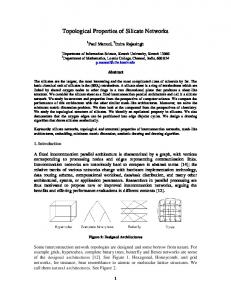
Interconnection network is a programmable system that transports data between terminals. Early work on interconnection networks was motivated by the needs of the communications industry, particularly in the context of telephone switching. With the growth of the computer industry, applications for interconnection networks within computing machines began to become apparent. As interest in parallel processing grew, a large number of networks were proposed for processor to memory and processor to processor interconnection [10]. An interconnection network consists of a set of processors, each with a local memory, and a set of bidirectional links that serve for the exchange of data between processors. A convenient representation of an interconnection network is by an undirected graph G = (V, E) where each processor is a vertex in V and two vertices are connected by an edge if and only if there is a direct communication link between processors[10]. A few networks such as Hexagonal, Honeycomb, and grid networks, for instance, bear resemblance to atomic or molecular lattice structures. Honeycomb networks, built recursively using the hexagon tessellation [14,15,16], are widely used in computer graphics [11], cellular phone
base station [12], image processing [2], and in chemistry as the representation of benzenoid hydrocarbons [15] and Carbon Hexagons of Carbon Nanotubes [9]. Hexagonal networks are based on triangular plane tessellation, or the partition of a plane into equilateral triangles [3,12,16]. Hexagonal network represents a host cyclotriveratrylene with halogenated monocarbaborane anions [1] and Silicon Carbide [13]. Carbon nanotubes consist of shells of sp2-hybridized carbon atoms forming a hexagonal network, arranged helically within a tubular motif [1]. In this paper, we deal with silicate networks which was introduced recently; silicates are obtained by fusing metal oxides or metal carbonates with sand. Essentially all the silicates contain SiO4 tetrahedra. The corner vertices of SiO4 tetrahedron represent oxygen ions and the center vertex represents the silicon ion. Graph theoretically, we call the corner vertices as oxygen nodes and the center vertex as silicon node. See Figure 1. The minerals are obtained by successively fusing oxygen nodes of two tetrahedra of different silicates.
Figure 1: SiO4 tetrahedra where the corner vertices represent oxygen ions and the center vertex the silicon ion In this paper, we study the topological properties of silicate networks as it has been studied for other interconnection networks [2,3,5,8,10,14,16]. We study its structure and properties from the perspective of computer science. In order to compare the computational powers of silicate networks with the other similar mesh-like architectures, those architectures are embedded into silicates. We also look at the compound from the perspectives of chemistry. We study the topological structure of silicates. We identify an equilateral property of silicates and we partition the oxygen edges into edge disjoint cycles. We propose an addressing scheme of silicate networks and map the nodes of silicate networks onto a Cartesian plane to draw the silicate network aesthetically.
3
3
2
2
1
1
0
0
1 2 3
1 2 3 (3,2,-1)
3
(3,1,-2) (2,-1,-3)
(a)
(b)
2
(1,-2,-3)
1
(0,0,0)
0
Figure 2: Construction of Silicate Network SL(n) from honeycomb network HC(n)
1 2
2
Properties of Silicate Networks
A silicate network can be constructed in different ways. Here in this paper we describe the construction of a silicate network from a honeycomb network. Consider a honeycomb network HC(n) of dimension n. Place silicon ions on all the vertices of HC(n). Subdivide each edge of HC(n) once. Place oxygen ions on the new vertices. Introduce 6n new pendant edges one each at the 2-degree silicon ions of HC(n) and place oxygen ions at the pendent vertices. See Figure 2(a). With every silicon ion associate the three adjacent oxygen ions and form a tetrahedron as in Figure 2(b). The resulting network is a silicate network SL(n). The parameter n of SL(n) is called the dimension of SL(n). The graph in Figure 2(b) is a silicate network of dimension 2. Theorem 1: The number of nodes in SL(n) is 15n2 + 3n. The number of edges of SL(n) is 36n2. □ When all the silicon nodes are deleted from a silicate network, we obtain a new network which we shall call as an Oxide Network. An n-dimensional oxide network is denoted by OX(n). Theorem 2: The number of nodes in OX(n) is 9n2 + 3n. The number of edges of SL(n) is 18n2. □
3
Addressing the nodes of Silicate Networks
In order to study the properties of silicate networks, it is important to assign a unique identity id (coordinate) to each node of silicate network. First we shall propose a coordinate system that can be used to assign an id to each node of oxide network. Then we shall extend this coordinate system to silicate network. We shall adapt the coordinate system that was proposed for a honeycomb network by Stojmenovic [14] or a hexagonal network by Nocetti et al. [12]. Three axes, α, β and γ parallel to three edge directions and at mutual angle of 120 degrees between any two of them are introduced, as indicated in Figure 3. The three coordinate axes are α = 0, β = 0, and γ = 0 respectively. We call lines parallel to the coordinate axes as α-lines, β-lines and γ-lines. Here α = h and α = – k are αlines on either side of α - axis.
(-3,-3,0)
3
Figure 3: Coordinate System in Oxide Networks Lemma 1: In (α, β, γ) coordinate system, the three lines α = h, β = k, and γ = l intersect if and only if k = h + l. Proof: Since the α-lines are parallel to X-axis, the α-line “α = 0” is taken as the x-axis. Line α = h, h Z of OX(n) is mapped to y = h in the Cartesian system. A β-line β = k makes an angle 60o with X-axis and forms a y-intercept 2k in the Cartesian system. Thus line β = k, k Z is mapped to y = (tan 60o)x + 2k which is y = √3x + 2k. A γ-line γ = ℓ makes an angle 120o with X-axis and forms a y-intercept – 2ℓ in the Cartesian system. Thus line γ = ℓ, ℓ Z is mapped to y = (tan 120o)x – 2ℓ which is y = – √3x – 2ℓ. See Figure 3. The lines α = h, β = k, and γ = l intersect the third line passes through the point of intersection of the first two lines y = h passes through the point of intersection of y = √3x + 2k and y = – √3x – 2ℓ. k l ,k l y = h is satisfied by 3 h = k – ℓ i.e., k = h + ℓ.□ Lemma 2: (α, β, γ) represents an oxide molecule if and only if (1) β = α + γ and (2) at least one of α, β, γ is odd. Proof: The proof is obvious. See Figure 3. □ The above lemma can also be restated as A node of OX(n) is assigned a triple (a, b, c) when the node is the intersection of lines α = a, β = b, and γ = c and at least one of a, b, c is odd. Remark: In an oxide molecule, exactly two of α, β, γ must be odd. Each silicon node is at the centroid of three oxygen nodes of a tetrahedral SiO4. Thus it is enough to specify an addressing scheme for the oxygen nodes of SL(n). For all practical purposes, we don’t need separate id for silicon
nodes since the silicate network is completely characterized by the oxide network. However for the sake of completeness, one can assign ids to silicon nodes by applying the formula of centroid of a triangle.
4
The edge set of OX(n) is partitioned into edge disjoint cycles
Definition: An edge of OX(n) is called α-edge if it is in some α-line. A β-edge and a γ-edge are defined in the same way. A cycle of OX(n) is said to be a symmetric cycle if it is formed by an α-edge, a β-edge and a γ-edge alternatively. Notice that the number of edges of any symmetric cycle of OX(n) is a multiple of 3. We demonstrate that the edge set of OX(n) is partitioned into edge-disjoint symmetric cycles. Theorem 3: The edge set of OX(n) can be partitioned into edge-disjoint symmetric cycles. Proof: As a strategy to partition the edge set of OX(n), we orient the edges of OX(n) as follows: Orient the edges of lines α = 1, 3 … 2n + 1 in the positive direction. Orient the edges of lines α = –1, –3 … –2n – 1 in the negative direction. Orient the edges of lines β = 1, 3 … 2n + 1 in the positive direction.
5
Equilateral Triangle Property of Silicate Network
Three vertices u, v, w of a graph G(V, E) are said to form an equilateral triangle if d(u, v) = d(v, w) = d(w, u) where d(x, y) denotes the distance between x and y. There is an interesting equilateral triangular property of silicate networks. Theorem 4: Three vertices A(x1, x2, x3), B(y1, y2, y3) and C(z1, z2, z3) of SL(n) form an equilateral triangle if x1 = y1, y2 = z2 and z3 = x3. □ Continuing the above theorem, we discuss a stronger result. Consider a triangle ABC formed by some α-line, β-line and γ-line. By the above theorem, ΔABC is equilateral. Let a1, a2 … ar be the nodes on the β-line between B and C. Let b1, b2 … br be the nodes on the α-line between C and A. Let c1, c2 … cr be the nodes on the γ-line between A and B. See Figure 5. We know that d(A, B) = d(A, C). The interesting observation is that d(A, B) = d(A, ai) = d(A, C) for i = 1, 2 … r. Theorem 5: Let ΔABC denote a triangle of SL(n) formed by three vertices A(x1, x2, x3), B(y1, y2, y3) and C(z1, z2, z3) such that x1 = y1, y2 = z2 and z3 = x3. Let a be a node on the β-line between B and C, let b be a node on the α-line between C and A and let c be a node on the γ-line between A and B. Then d(A, B) = d(B, C) = d(C, A) = d(A, a) = d(B, b) = d(C, c). □
Orient the edges of lines β = –1, –3 … –2n – 1 in the negative direction. Orient the edges of lines γ = 1, 3 … 2n + 1 in the positive direction.
b4
b3
b2
b1
C
A c1
Orient the edges of lines γ = –1, –3 … –2n – 1 in the negative direction.
a4 a3
c2 c3
a2 c4
a1 B
Figure 5: Equilateral triangle property
6 Figure 4: Edge set of OX(n) is partitioned into cycles See the orientation in Figure 4. Symmetric cycles in the oriented OX(n) are unique. Hence it is now easy to partition OX(n) into edge-disjoint symmetric cycles. The innermost symmetric cycle is a hexagon of the length 6. Then onwards, each successive symmetric cycle forms a layer on the previous one. See Figure 4. The length of each symmetric cycle is a multiple of 6. □
Embedding of Honeycomb and Hexagonal Networks in Silicate Networks
Let G and H be finite graphs with n vertices. V(G) and V(H) denote the vertex sets of G and H respectively. E(G) and E(H) denote the edge sets of G and H respectively. An embedding [10] f of G into H is defined as follows: 1. f is a bijective map from V(G)→V(H). 2. f is a one-to-one map from E(G) to {Pf(f(u),f(v)) / Pf(f(u),f(v)) is a path in H between f(u) and f(v), (u,v) E(G)}.
The dilation Dˆ f (G, H ) of an embedding f of G into H is defined as Dˆ f (G, H ) max | Pf ( f (u ), f (v)) |
1
2
3
4
1
7
5 11
12
10
9 13
14
18
5
24
25
6
3
1
4
6
18 24
14
15
33
34
25
22
26
27 28
29
31
37 35
20
23
31
33 36
35
36
34
37
Figure 8: Hexagons of HX(n) between successive α = 2k + 1 and α = 2k + 3 lines are mapped into the corresponding hexagons of SL(n – 2). 6
6
8
8
19
17 17
19
21
21
32
30 32
30
Figure 9: Center node of the hexagon of HX(n) is mapped into a node which sits on top of the corresponding hexagon of SL(n – 2)
3
4
5
9 13
27
29
2
2
16
28
f
1
26
23
Then, the dilation of G into H is defined as Dˆ (G, H ) min Dˆ (G, H ) where the minimum is taken over all embeddings f of G into H. The dilation problem for a graph G into H is that of finding an embedding of G into H that induces the dilation Dˆ (G, H ) . We next state the results pertaining to embedding of honeycomb and hexagonal networks into silicate networks. Theorem 6: The dilation of the embedding of a honeycomb network of dimension n into a silicate network of the same dimension is 2. Proof: From the structure of SL(n) described in Section 3, it follows that the subdivision of the honeycomb network of dimension n is a subgraph of SL(n). See Figure 6. Hence the dilation of the embedding of HC(n) into SL(n) is 2. □
7 12
11
20 22
where |Pf(f(u),f(v))| denotes the length of the path Pf(f(u),f(v)).
4
3
15 10
( u ,v )E ( G )
2
5
1
2 6
5 11
12
10 16
3
17
4
1
8
7 13 18
9 14
19
10
25
8
3
4
7 12
11
16
18
9 13
14
15
20
20 21
24
2
5 15
15 23
6
26
15
17
27
22
23
28
30
19 24
25
32
21 26
27 28
22
Figure 6: Dilation of the embedding is 2 Theorem 7: The dilation of the embedding of HX(n) into SL(n – 2) is at most 3. Proof: We provide an embedding of HX(n) into SL(n – 2) as follows: Step 1: The nodes of HX(n) are labeled along α –lines from left tot right as in Figure 7. Step 2: Each hexagon of HX(n) between successive α = 2k + 1 and α = 2k + 3 lines is mapped into the corresponding hexagon of SL(n – 2). See Figure 8. Step 3: The center node of a hexagon of HX(n) is mapped into a node which sits on top of the corresponding hexagon of SL(n – 2). See Figure 9. The Figure 10 shows the embedding of HX(n) into SL(n – 2). It is easy to verify that the dilation of this embedding is 3. □ 1
2 6
5 11
18
4 8
7 12
10 17
3
13 19
9 14
20
15 21
16
22 24
25
26
27
23
28 31
30
32
29
33
34
37 35
36
Figure 7: The nodes of Hexagon HX(n) are labeled
31
30
32
29
33 35 34
36
29
31 35
37 34
33 36 37
Figure 10: An embedding of HX(n) into SL(n – 2). The edge (6, 11) of HX(n) is dilated along 6, 1, 5, 11 in SL(n – 2). The dilation of HX(n) into SL(n – 2) is 3. Thus algorithms such as minimum communication cost, routing, and broadcasting algorithms of honeycomb and hexagon networks [5, 8, 10] can be simulated in silicate networks with a time complexity that differ by a constant.
7
More Properties of Silicate Networks
Theorem 8:
(i) OX(n) contains a Hamiltonian path. (ii) SL(n) contains a Hamiltonian path. Proof: (i) By the method of induction. OX(1) contains a Hamiltonian path. See Figure 11 (a). Assume the theorem is true for OX(k). i.e., OX(k) has a Hamiltonian path. To prove the theorem is true for OX(k + 1). By theorem 3, The edge set of OX(n) is partitioned into edgedisjoint symmetric cycles. By induction, there exists a Hamiltonian path in OX(k). This path is connected to the outermost symmetric cycle thus producing a Hamiltonian path in OX(k+1). See Figure 11 (b)
(ii) The proof of (ii) is similar to the above proof as the path v1 not have the same color. Since no two nodes on = … –4, – v2 v3 is replaced by v1 v2 v4 v3. See Figure 12 (a) and 12 (b). □ 2, 0, 2, 4 … are adjacent and each node on these -lines is adjacent to nodes colored yellow and blue, (OX (n)) 3. Since the chromatic number of a triangle is 3, (OX (n)) 3. Thus (OX (n)) = 3 and hence OX(n) is tripartite. □ Remark: (i) SL(n) is not bipartite since it contains odd cycles. (ii) OX(n) is Eulerian but SL(n) is not Eulerian since it contains odd degree vertices. Domatic Number: A dominating set in a graph is a set of vertices such that every vertex in the graph is either in the set (a) (b) or has a neighbour in the set. A domatic partition is a partition of the vertices so that each part is a dominating set Figure 11: Hamiltonian path in OX(1),and OX(2) of the graph. The domatic number of a graph G denoted by D(G) is the maximum number of dominating sets in a domatic partition of the graph G, or equivalently, the maximum number of disjoint dominating sets[4]. The domatic partition problem is that of partitioning the vertices of a graph into the maximum number of disjoint dominating sets. The domatic partition problem is one of the classical NP – hard problems [7]. Lemma 1 [4]: Every graph G satisfies D(G) 1, and unless Figure 12: (a) A Hamiltonian path in a triangle of OX(n), G contains an isolated node, D(G) 2. (b) A Hamiltonian path inside a triangle of SL(n), Lemma 2 [4]: Let denote the minimum degree of a node (c) A Hamiltonian path in SL(2). in the graph G. Then D(G) + 1. Remark: Using exhaustive MATLAB simulation, we Proof: Since the node with minimum degree must have some observe that OX(n) has no Hamiltonian cycle. However there neighbor (or itself) in each of the disjoint dominating sets, is no mathematical proof to show that OX(n) has no D(G) + 1. □ Hamiltonian cycle. It is interesting to derive a logical proof to Theorem 10: (i) The domatic number of OX(n) is 3. show that OX(n) has no Hamiltonian cycle. (ii) The domatic number of SL(n) is 4. Theorem 9: Proof: By Lemma 2, D(OX(n)) 3 and D(SL(n)) 4. (i) OX(n) is tripartite and its chromatic number is 3. (ii) SL(n) is 4-partite and its chromatic number is 4. 3
3
2
2
1
1
0
0
1 2 3
1 2 3
(3,2,-1)
3
(3,1,-2) (2,-1,-3) (1,-2,-3) (0,0,0)
2
1
0 1
(a)
2
(-3,-3,0)
(a)
(b)
Figure 14: (a) Domatic coloring for OX(2), (b) Domatic coloring for SL(2)
3
(b)
Figure 13: (a) Coordinate System in Oxide Networks, (b) Chromatic coloring for OX(2) Proof: Claim that the chromatic number (OX (n)) is 3. See Figure 13. Label the nodes on the - lines corresponding to = … –4, –2, 0, 2, 4 … by color 1 (red). Label the nodes on the - lines corresponding to = … –3, –1, 1, 3, 5 … by color 2 (yellow) and color 3 (blue) such that adjacent nodes do
We have presented in Figure 14, a domatic partition of size 3 for OX(n) and size 4 for SL(n). Therefore D(OX(n)) 3 and D(SL(n)) 4. □
8
Drawing Algorithm for Silicate Networks
Let us classify the edges of a tetrahedral SiO4 as follows: An edge incident at a silicon node is called silicon edge. Otherwise it is called an oxygen edge. The drawing algorithm
provides a method to draw SL(n) in the Cartesian plane. That is, it provides a formula to map a node (α, β, γ) of SL(n) into a point (x, y) of Cartesian System. Our objective is to draw SL(n) in Cartesian plane in such a way that all the drawn edges of SL(n) are of equal length in the 2-dimnesional plane. However, it is not possible to draw a tetrahedral SiO4 (a complete graph on 4 vertices) in the 2-dimensional plane such that all edges are of equal length. Therefore, we design a drawing algorithm such that all the silicon edges are of the same length and all the oxygen edges are of the same length. As mentioned earlier, it is enough to design a drawing algorithm for oxide network. The oxygen edges of a tetrahedral SiO4 form a triangle. In other words, these three oxygen edges should make an equilateral triangle in order to be of equal length. Geometrically, these three edges make an angle of 60o with each other. Moreover, these three oxygen edges are on α-lines, β-lines, and γ-lines of OX(n) respectively. In order to keep all the oxygen edges of equal length, α-lines, β-lines, and γ-lines of OX(n) are drawn as follows: All α-lines are parallel to X-axis, β-lines make 60o with X-axis and γ-lines make 120o with X-axis. Successive α-lines (β-lines, and γ-lines) are equally spaced in the Cartesian plane. (1) Since the α-lines are parallel to X-axis, the α-line “α = 0” is taken as the x-axis. Line α = (2h+1), h Z of OX(n) is mapped to y = (2h+1) in the Cartesian system. (2) A β-line β = (2k+1) makes an angle 60o with X-axis and forms a y-intercept 2(2k+1) in the Cartesian system. See Figure 3. Thus line β = (2k+1), k Z is mapped to y = (tan 60o)x + 2(2k+1) which is y = √3x + 2(2k+1). (3) A γ-line γ = (2ℓ+1) makes an angle 120o with X-axis and forms a y-intercept – 2(2ℓ+1) in the Cartesian system. See Figure 3. Thus line γ = (2ℓ+1), ℓ Z is mapped to y = (tan 120o)x – 2(2ℓ+1) which is y = – √3x – 2(2ℓ+1). From (1), we have α = (2h+1) and y = (2h+1), h Z Thus y = α. (A) From (2) and (3) we have β = (2k+1) and y = √3x + 2(2k+1). γ = (2ℓ+1) and y = – √3x – 2(2ℓ+1). Solving the above two equations, we get x = – (β + γ)/√3. (B) Combining (A) and (B), we arrive at a function f that maps a node (α, β, γ) of OX(n) to a node of Cartesian System as follows: f(α, β, γ) = (– (β + γ)/√3, α). (C) This function f provides an algorithm to draw OX(n) in a Cartesian plane. Once the oxide network is drawn in the Cartesian plane, placing silicon nodes is rather simple. As we know, a silicon node is at the centroid of three oxygen nodes of a tetrahedral SiO4. If (x1, y1), (x2, y2), (x3, y3) are the Cartesian coordinates of oxygen nodes of a tetrahedral SiO4, then ((x1+x2+x3)/3, (y1+y2+y3)/3) is the Cartesian coordinate of the silicon node
of the tetrahedral SiO4. This completes the drawing algorithm of SL(n). Theorem 11: A silicate network can be drawn in a twodimensional Cartesian plane such that all the silicon edges are of equal length and all the oxygen edges are of equal length. □ 8.1
MATLAB program to draw SL(n)
function silicate(n) close all;axis square;hold on T=0:0.01:1; rad1=0.07; for i=-2*n:2*n for j=-2*n:2*n for k=-2*n:2*n if (j-k == i && (mod(i,2)~=0 || mod(j,2)~=0 || mod(k,2)~=0)) fill(-(j+k)/sqrt(3)+rad1*cos(2*pi*T), i+rad1*sin(2*pi*T),'b') if (mod(i,2)==0 && i~=2*n) for t = -1:1 if t~=0 fill(-(j+1/3+k-1/3)/sqrt(3)+rad1*cos(2*pi*T), t*(i+2/3)+rad1*sin(2*pi*T),'r') plot([-(j+1/3+k-1/3)/sqrt(3) -(j+k)/sqrt(3)], [(i+2/3) i],'b') plot([-(j+1/3+k-1/3)/sqrt(3) -(j+1+k)/sqrt(3)], [(i+2/3) i+1],'b') plot([-(j+1/3+k-1/3)/sqrt(3) -(j+k-1)/sqrt(3)], [(i+2/3) i+1],'b') plot([-(j+1/3+k-1/3)/sqrt(3) -(j+k)/sqrt(3)], [-(i+2/3) -i],'b') plot([-(j+1/3+k-1/3)/sqrt(3) -(j+1+k)/sqrt(3)], [-(i+2/3) -(i+1)],'b') plot([-(j+1/3+k-1/3)/sqrt(3) -(j+k-1)/sqrt(3)], [-(i+2/3) -(i+1)],'b') end end end end end end end for i=1:n for j = -1:1 if j~=0 plot([(4*(n-1)+3-2*(i-1))/sqrt(3) -(4*(n-1)+3-2*(i-1))/sqrt(3)], [j*(2*i-1) j*(2*i-1)]) plot([j*(4*(n-1)+3-2*(i-1))/sqrt(3) j*(2*(n-1)-4*(i-1))/sqrt(3)], [-(2*i-1) 2*n]) plot([j*(4*(n-1)+3-2*(i-1))/sqrt(3) j*(2*(n-1)-4*(i-1))/sqrt(3)], [(2*i-1) -2*n]) end end end hold off
Parallel and Distributed Systems, vol. 5, no. 1, pp 31-38, 1994. [6] Gamst A, Homogeneous Distribution of Frequencies in a Regular Hexagonal Cell System, IEEE Transactions on Vehicular Technologies, vol. 31, pp 132-144, 1982. [7] M. R. Garey and D. S. Johnson, Computers and Intractability: A gude to the Theory of NP – completeness. Freeman. 1979. [8] Hamid Reza Tajozzakerin, Hamid Sarbazi-Azad, Enhanced-Star: A New Topology Based on the Star Graph, LNCS, vol. 3358, pp 1030-1038, 2005.
Figure 15: Silicate drawn using MATLAB
9
Conclusion
In this paper we have considered a new interconnection network motivated by the molecular structure of certain chemical compounds. We have investigated the topological and structural properties of this network. We have provided an addressing scheme for the nodes of the network and also an algorithm that enables us to draw the silicate network in the two dimensional plane aesthetically. It is shown that any algorithms such as minimum communication cost, routing, and broadcasting algorithms of honeycomb and hexagon networks can be simulated in silicate networks with a time complexity by a difference of constant factors. This paper is an eye opener for researchers in the sense that different networks can be derived using the ores and compounds available in nature.
10 References [1] Ahmad R, Franken A, Kennedy J. D, Hardie M. J, Group 1 Coordination Chains and Hexagonal Networks of Host Cyclotriveratrylene with Halogenated Monocarbaborane Anions, Chemistry, vol. 10(9):2190-8, May 3, 2004. [2] Bell S. B. M, Holroyd F. C, Mason D. C, A Digital Geometry for Hexagonal Pixels, Image and Vision Computing, vol. 7, pp 194-204, 1989. [3] Catherine Decayeux, David Seme, 3D Hexagonal Network: Modeling, Topological Properties, Addressing Scheme, and Optimal Routing Algorithm, IEEE Transactions on Parallel and Distributed Systems, vol. 16, no. 9, pp 875884, 2005. [4] E.J. Cockayne and S. Hedetniemi, Towards a theory of domination in graphs. Networks 7 (1977), 247-261. [5] Day K, Tripathi A, A Comparative Study of Topological Properties of Hypercubes and Star Graphs, IEEE Transactions on
[9] Hongwei Zhu, Kazutomo Suenaga, Jinquan Wei, Kunlin Wang, Dehai Wu, Atom-Resolved Imaging of Carbon Hexagons of Carbon Nanotubes, J. Phys. Chem. C, vol. 112, no. 30, pp 11098-11101, 2008. [10] Junming Xu, Topological Structure and Analysis of Interconnection Networks, Kluwer Publishers, 2001. [11] Lester L. N, Sandor J, Computer Graphics on Hexagonal Grid, Computer Graphics, vol. 8, pp 401-409, 1984. [12] Nocetti F.G, Stojmenovic I, Zhang J, Addressing and Routing in Hexagonal Networks with Applications for Tracking Mobile Users and Connection Rerouting in Cellular Networks, IEEE Transactions On Parallel And Distributed Systems, vol. 13, no. 9, pp 963-971, September 2002. [13] Paul Manuel and Indra Rajasingh, Minimum Metric Dimension of Silicate Networks, Ars Combinatoria (volume 98, January 2011). [14] Stojmenovic I, Honeycomb Networks: Topological Properties and Communication Algorithms, IEEE Trans. Parallel and Distributed Systems, vol. 8, pp 1036-1042, 1997. [15] Tosic R, Masulovic D, Stojmenovic I, Brunvoll J, Cyvin B. N, Cyvin S. J, Enumeration of Polyhex Hydrocarbons up to h = 17, Journal of Chemical Information and Computer Sciences, vol. 35, pp 181-187, 1995. [16] Wenjun Xiao, Behrooz Parhami, Further Mathematical Properties of Cayley Digraphs Applied to Hexagonal and Honeycomb Meshes, Discrete Applied Mathematics, vol. 155, no. 13, pp 1752-1760, 2007.