Abstract. We study the adaptive behavior of a computational ecosystem in the presence of time-periodic resource utilities as seen, for example, in the dayânight ...
Computational Ecosystems in a Changing Environment Natalie Glance, Tad Hogg and Bernardo A. Huberman Intl. J. of Modern Physics C 2, 735–753 (1991) Abstract We study the adaptive behavior of a computational ecosystem in the presence of time-periodic resource utilities as seen, for example, in the day–night load variations of computer use and in the price fluctuations of seasonal products. We do so within the context of the Huberman-Hogg model of such systems. The dynamics is studied for the cases of competitive and cooperative payoff functions with time-modulated resource utilities, and the system’s adaptability is measured by tracking its performance in response to a time-varying environment.
Keywords: non-linear dynamics, distributed computation, adaptability.
1
Introduction
Social conventions and the cycles of nature make for periodic variations in the prices of commodities and resources. The use of computers in the workplace, for example, tends to be high during the day but low at night, a pattern that is also found in terms of workdays and weekends. This pattern is reflected in the variation of the availability of the machines beyond the individual’s control. Similarly, seasonal outputs in agriculture modulate the availability of goods in ways that are usually reflected in their price variation across the year, and the familiar cycles of electricity consumption and phone use lead to pricing structures that exploit their periodicity. Although it may be easy to predict the influence of such fluctuations on isolated agents, it is generally much harder to determine the global response of a large system consisting of many autonomous agents making local decisions. Nevertheless, it is the aggregate behavior of a system of agents that determines important characteristics such as system performance and adaptability to a changing environment. Distributed systems arise in many different contexts including computation [3, 5, 9], biological ecosystems [8], economies, and social structures [10]. A computational ecosystem [6] is a type of distributed computation in which independent agents vie for limited resources. These ecosystems embody several characteristics of distributed systems including distributed control, asynchrony in execution, resource contention, and cooperation among agents, and also suffer from the concomitant problems of incomplete knowledge and delayed information. The dynamics of such systems has been studied in detail and tested experimentally [7] to ascertain the behavior of computational agents choosing among available resources. It was found that when the perceived payoff associated with particular resources depends on the number of agents choosing them, the resulting behavior ranges from simple fixed points to nonlinear oscillations and chaos with the ensuing decrease in the overall performance of the system. The previous work did not examine the more realistic case that includes unavoidable time-dependent variations in the environment. Introducing a time-modulated fluctuation to the payoffs captures the effect of such a changing environment. Apart from this specification, this paper will remain faithful to the original Huberman-Hogg theory in all aspects, and, in particular, the agents are taken to be unable to perceive patterns in either the behavior of the other agents or in the external environment. In general, the environment can vary in unpredictable and often uncontrollable ways. Allowing the payoff functions to vary similarly would produce results that would be very difficult to interpret. (Also, it should be noted that a simple random zero-mean uncorrelated fluctuation is already included in the theory to model information uncertainty.) However, a simple sinusoidal modulation should capture many of the pertinent
1
effects. It is expected from analogy with driven oscillators [4] that the interplay between the frequency of the global utility variation and those of an intrinsically nonlinear system will in principle allow for rich dynamical behavior that should be elucidated. Study of computational ecosystems within a changing environment also sheds light on the issue of adaptability. What are the characteristics of an adaptable system, and is it possible to predict its adaptability from knowledge of the underlying dynamics? These questions are important since the existence of a stable equilibrium for an isolated computational ecosystem does not imply that the system is adaptive. This stems from the possibility that the system’s very stability may prevent it from adjusting to time-dependent constraints. In the following, we begin by summarizing the model of computational ecosystems and then perform a mathematical analysis of the underlying equations to determine the effect of time-modulation on dynamical stability in various limits. When analytic methods fail us, we turn to computer experiments for help in mapping the behavioral regimes of a system with both competitive and cooperative payoffs. Finally, we address the question of adaptability, defining a measure of performance which we use to describe how well a set of agents and resources is able to adapt to a time-varying environment.
2
The Model
We consider a simple system composed of identical agents competing for two resources. We assume that the agents prefer a resource solely on the basis of its perceived payoff. These payoffs are actual computational measures of the resources’s performance, such as the time required to complete a task, accuracy of the solution, amount of memory required, etc. In addition, the information the agents have is imperfect and delayed in time. Imperfect information causes each agent’s perceived payoff to differ somewhat from the actual value, with the difference increasing when there is more uncertainty in the information available to the agents. This simple model of uncertainty concisely captures the effect of many sources of errors such as some program bugs, heuristics incorrectly evaluating choices, errors in communicating the load on various machines and mistakes in interpreting sensory data. Lastly, information delays cause each agent’s knowledge of the state of the system to be somewhat out of date. As shown in [6], the time-evolution of the fraction of agents using resource 1 is described within the mean-field approximation by the differential-delay equation [2] df1 (t) = −α (f1 (t) − ρ(f1 (t − τ ))) dt
(1)
where ρ(f ) is the probability that a single agent will choose resource 1 if a fraction f of the agents is already using it, with α the average rate at which agents reevaluate their choices and τ the delay. In terms of the density-dependent payoff functions for using resources 1 and 2, G1 (f1 (t)) and G2 (f1 (t)) and the uncertainty σ characterizing the size of the errors in the agents’ perceptions, ρ is given by µ µ ¶¶ G1 (f1 (t)) − G2 (f1 (t)) 1 1 + erf (2) ρ(f1 ) = 2 2σ The fraction of agents using resource 2 is then simply 1 − f1 (t). The nature of the interactions among agents determines how the payoff functions depend on the fraction of agents using particular resources. In a purely competitive environment, the payoff for using a particular resource would decrease as more agents make use of it. Alternatively, the agents using a resource could assist one another in their computations, as might be the case if the overall task could be decomposed into a number of subtasks. If these subtasks communicate extensively to share partial results, the agents might be better off using the same computer rather than running more rapidly on separate machines but then being limited by slow communications. As another example, agents using a particular database could leave index links that are useful to others. In such cooperative situations, the payoff of a resource would increase as more agents use it, at least until it became sufficiently crowded. A more general scenario combines the two effects of competition and cooperation, giving rise to a payoff function which at first increases as the number of agents using the resource increases but eventually saturates. The simplest example of this is a payoff for using a resource which reaches a maximum somewhere in the interval 0 < f < 1 instead of 2
decreasing monotonically with increasing f as would be the case if the interactions were mostly competitive. For simplicity, we refer to the last example given as the cooperative case. Two different choices of payoff functions corresponding to competitive and cooperative systems have been studied in detail [7]. The competitive payoffs considered were given by G1
=
G2
=
7 − f1
(3)
7 − 3f2
For this situation, the dynamics of the undriven system is well-understood. For a given uncertainty σ, β = ατ is varied to obtain three types of behavior: (1) exponential decay to the fixed point, f eq , given by ρ(feq ) = feq ; (2) damped oscillations about feq ; and (3) persistent oscillations. The behavioral phase diagram for this system given in Fig. 1(a). The case of a system of cooperating agents with the following payoff functions was also studied [7]: G1
=
G2
=
4 + 7f1 − 5.333f12
(4)
7 − 3f2
The payoffs were chosen to have the same fixed point as for the competitive case when there is no uncertainty. This combination of agents and resources exhibits stability, instability, bifurcation, and chaos for different choices of β and σ (see behavioral phase diagram given in Fig. 1(b)). (a)
(b)
2
1.0
σ
Damped Oscillations
0.8
Damped Oscillations
0.6
Persistent
σ
1
Oscillations 0.4
Period Doubling
0.2
Persistent
Chaos
Oscillations 2.5
0
5
2
6
4
8
10
β
β
Figure 1: Behavioral phase diagram as a function of β = ατ and uncertainty parameter σ for an undriven system of identical agents with the competitive payoffs of Eq. (3) in (a); with the cooperative payoffs of Eq. (4) in (b). In the unshaded regions, the system exhibits overdamped (non-oscillatory) relaxation to the fixed point. The chaotic region in (b) is punctuated by numerous windows of periodic behavior (not shown). Results were obtained by analysis and by integrating Eq. (1) numerically. In the previous examples, G1 and G2 depend only on f1 and f2 , and only indirectly upon time. To investigate the behavior of this model within a changing environment, we now take the basic capacity of one of the resources to vary sinusoidally in time. This models the effect, for example, of the variation from day to night on the load of a network of computers. This load is considered to be a cumulation of effects external to the ecosystem. Specifically, we introduce an explicit time-dependence for the utility of resource 1, say, by taking G1 (f1 ) → G1 (f1 ) + A sin ωt (5)
with A the amplitude and ω the frequency of the sinusoidal variation in the payoff of resource 1. This models changes in the resource’s base capacity taken to be independent of the agents’ actions. Note that since the payoffs for using the two resources enter into the equations describing the evolution of the ecosystem only through their difference, G1 − G2 , in the case of two resources, time-modulating the payoff of one or the other leads to identical results. This will not remain true if we consider more than two resources. Lastly, we remark on a notational convenience adopted for the remainder of the paper. In order to make explicit the functional dependence of the probability ρ on the driving term u ≡ A sin ωt, we will refer to the probability ρ by ρ(f, u) or, alternatively, ρ(f, A), when the frequency is irrelevant to the discussion. 3
3
Driving a Stable System
We will now examine the behavior of the agents in the case where the undriven system is stable.
3.1
Small amplitudes
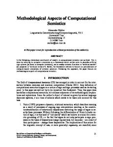
In the limit of very small amplitude oscillations in the resource utilities (i.e., A much smaller than the typical difference between the payoffs G1 and G2 ), we expect the effects of the driving term to vanish. As a result, we consider the solution in which the system oscillates at the driving frequency about the equilibrium value feq , which is given by feq = ρ(feq , A = 0) (6) We can obtain the conditions under which such oscillations are stable by linearizing Eq. (1) in the neighborhood of the fixed point feq and about A = 0. Defining the variation around the fixed point as δ(t) = f (t)−f eq , we obtain dδ + α(δ(t) − γδ(t − τ )) = αηA sin ω(t − τ ) (7) dt where γ = ρf (feq , A = 0) and η = ρu (feq , A = 0) are the partial derivatives of ρ with respect to f and u, the latter being u = A sin ωt. The solution to this inhomogeneous differential–delay equation [2] consists of the sum of the particular solution, δ(t) = B sin(ωt + φ), where both B and φ depend in a complicated fashion upon A, α, τ , and σ, and the solution to the homogeneous equation dδ dt + α(δ(t) − γδ(t − τ )) = 0. Since the particular solution remains small (B → 0 as A → 0), the stability of Eq. (7) is determined by the behavior of the homogeneous equation, which was previously studied in the context of time-independent resource utilities [7]. The results of that analysis are displayed in Fig. 1, which shows the oscillation and stability thresholds for two different sets of payoffs (competitive and cooperative) in the undriven case. Since in the presence of a driving term the system is stable for the same parameter values, we can use these results to ascertain the behavior of the driven system in the parameter region corresponding to the existence of a fixed point. Thus, relaxation to a fixed point of the undriven system maps into tracking of the time-dependent variation with some phase shift dependent on both α and τ , and with the same stability boundaries as the undriven system. This can be seen in the oscillation of f (t) at the driving frequency with a phase lag, as shown in Fig. 2. (Undriven, the system relaxes to a fixed point.) In this case the phase lag between the driving signal and the response of the system is 1.45 time units, significantly smaller than the delay, which equals three time units. Since the phase lag can vary from 0 to 2π (depending on the value of the delay and the reevaluation rate), this result indicates the system’s inability to track the time variation in the relative payoffs between the resources.
3.2
High amplitudes
In the limit of high amplitude Eq. (1) is exactly solvable. If A is much greater than the typical difference between the payoffs G1 and G2 , the value of ρ(f, u = A sin ωt) is determined to zeroth order by the sign of the sine function. Thus, when sin(ωt) is positive ρ = 1, and f (t) relaxes exponentially towards one, whereas when sin(ωt) becomes negative ρ = 0, and f (t) decays exponentially to zero. However, since ρ is evaluated at t − τ , not at t, the switching between growth and decay will lag the driving term by an amount equal to the delay τ . While this analysis is only a zeroth order solution, numerical integration of Eq. (1) corroborates its validity. Fig. 3 shows the typical response of the system when there is a large amplitude modulation of the utilities for a system with two resources. Here the oscillation lags the driving frequency by τ . In closing, we mention that as in the previous case of low amplitudes, f (t) can oscillate 180 ◦ out of phase with the driving term, with the resultant loss of tracking. Such behavior holds everywhere in the behavioral phase diagram of computational ecosystem (i.e., for all values of uncertainty, delay, and reevaluation rate).
3.3
Intermediate amplitudes
If the resource utilities are driven at some frequency ω for intermediate amplitudes, we expect that parameters which yielded fixed points in the undriven system will lead to oscillations with the same frequency and with
4
f(t) 0.68
0.66
0.64
0.62
360
370
380
390
400
t
Figure 2: Example of low-amplitude driving. Dark curve shows fraction of agents f (t) using resource 1 (≡ f 1 (t)) with competitive payoffs of Eq. (3) when driven at frequency ω = 1, low amplitude A = 0.1, for parameters α = 1, τ = 3, σ = 0.9. Notice that f remains close to the fixed point of the undriven system, f eq = 0.64. Light curve shows phase of driving term and its scale is irrelevant and unrelated to amplitude of driving term. f(t) 1
0.8
0.6
0.4
0.2
10
20
30
40
50
t
Figure 3: Example of high amplitude modulation of the resource utilities. Dark curve shows fraction of agents f (t) using resource 1 with competitive payoffs of Eq. (3) when driven at frequency ω = 0.5, high amplitude A = 100, for parameters α = 1, τ = 1, σ = 0.5. Light curve shows phase of driving term and again its scale is unrelated to amplitude of driving term.
some phase shift. This simply entails extrapolating from the analytical results for the low and high amplitude limits to intermediate amplitudes. As we saw, for both high and low amplitudes the stable region of the undriven system maps onto oscillatory behavior at the driving frequency with some phase lag. Lack of tracking of external driving therefore occurs even in parameter regions corresponding to stable behavior for the undriven system. Note that in the high amplitude limit, the phase lag is determined by τ , while for very low amplitudes the phase lag depends both on α and τ in a non-trivial way. Thus, in general, the dynamics of the system depends on both α and τ independently, not only on their product, unlike the case of the undriven system which can be characterized by the parameter β = ατ . Fig. 4 shows the fraction of agents using resource 1 vs. time when the relative payoffs of the two resources are modulated at a frequency ω = 1 with amplitude A = 1. This is shown superimposed upon the sinusoidal 5
driving term, making apparent the phase difference between them. The phase difference in this case equals 1.55 time units. Notice that at first the phase lag between the driving term and the behavior of the agents is about one delay period (which is only to be expected since it takes the system one delay period to observe the signal); as the system settles into equilibrium behavior, however, the lag decreases to the value stated above. f(t)
0.9
0.8
0.7
0.6
0.5
0.4
0.3
10
20
30
40
50
t
Figure 4: Competitive system of agents driven within parameter region corresponding to damped oscillation region of undriven system. Dark curve shows fraction of agents f (t) using resource 1 for competitive payoffs of Eq. (3) when driven at frequency ω = 1, intermediate amplitude A = 1, for parameters α = 1, τ = 3, σ = 0.9. Light curve shows phase of driving term (scale is unrelated to amplitude of driving). We can obtain further insights into the behavior of the system at intermediate amplitudes through study of the low and high frequency limits, to which we now turn.
3.4
The low frequency limit
In the limit of very low frequency time-modulation of one of the resource payoffs, some analytic results can be obtained. As long as the period of driving is much longer than both the delay and 1/α, i.e., 1/ω À 1/α, τ , the behavior over time intervals small compared with the period of oscillation of the payoff difference corresponds to the behavior found for the undriven case. Over longer time scales (on the order of 1/ω), the small time scale behavior is simply modulated by the low frequency driving. This can be shown by linearizing Eq. (1) about an equilibrium point feq (t), which is allowed to vary slowly in time, in the spirit of an adiabatic approximation. This equilibrium is given by feq (t) = ρ(feq (t − τ ), A sin ω(t − τ ))
(8)
where τ ¿ 1/ω. Since feq (t), changes slowly, we use the approximation feq (t) ≈ feq (t − τ ) when solving for feq (t). Defining the variation around the time-dependent equilibrium value as δ(x) = f (x) − f eq (t) and using x as a rescaled time variable describing intervals much smaller than 1/ω, we obtain a differential equation describing the evolution of the variation δ(x) about the fixed point. This equation is valid for time scales short compared with 1/ω. Thus, we recover the familiar equation dδ = α(δ(x) − γ(t)δ(x − τ )) dx
(9)
where the time dependent variable γ is given by γ(t) = ρf (feq (t)) and changes slowly. This result indicates that the behavior of the agents is well-described by the behavioral phase diagrams given for the undriven cases; however, the stability thresholds shift in response to the driving. 6
If we choose a point in the phase diagram close to the stability threshold, we indeed find instances in which a low frequency modulation of the payoff difference takes the system across the stability threshold from an unstable regime into a stable regime and vice-versa. Fig. 5 portrays one such example. In this case, the choice of σ, α, and τ places the system right below the oscillation threshold for the undriven system of Fig. 1. Thus, a low frequency modulation of the payoffs changes the difference in payoffs G1 (t) − G2 (t) and shifts the oscillation threshold downwards. This shift continues for times long enough so that the behavior of the system stabilizes until the next upward shift of the stability boundary causes oscillations to appear anew. We have before us the amusing example of a system which is stable at night when network use is conventionally light and inexpensive, but unstable during the day when use is heavy. f(t) 1
0.9
0.8
0.7
0.6
0.5
25
50
75
100
125
150
175
200
t
Figure 5: Shifting of the oscillation threshold occurs when system is driven at low frequencies near the boundary between the damped oscillation and persistent oscillation regions. The figure shows the fraction of agents f (t) using resource 1 for competitive payoffs of Eq. (3) when driven at frequency ω = 0.1, amplitude A = 1, for parameters α = 1, τ = 1, σ = 0.4.
3.5
The high frequency limit
The case of high frequencies poses some interesting questions on how well the computational ecosystem model aligns with real distributed systems. If the environment varies at a rate much greater than the agents’ reevaulation rate, do the agents see an average of the variation over time scales comparable to 1/α or do they observe fluctuations that look like correlated noise? For the case of a sinusoidal modulation, the former case implies that the time-variation is not seen by the agents (zero mean), while the latter indicates that the resulting behavior might correspond to that of an undriven system with a renormalized value of the uncertainty. In order to address this issue we must reexamine how the agents obtain information about the resources. While the agents perform their evaluations asynchronously and independently, they could either accumulate information over discrete intervals of time or obtain it instanteneously. In our model, the agents are taken to act in the latter fashion. Thus, in the limit of an infinite number of agents which is taken in the mean-field approximation, during any short time interval many agents are gathering data about the various resources, and the very rapid modulation of the payoffs affects the system through its root–mean–square value, not through its average value. This remains true as the number of agents becomes finite, as long as there are a significant number of agent evaluations during one period of the very rapid modulation. Thus, we expect the mean-field equation to remain valid in the high-frequency limit of ω À α if N α À ω, where N is the total number of agents. Computer experiments verify the prediction that high-frequency modulation of the payoff utilities causes the system to behave as if the uncertainty were increased and the payoffs unmodulated, an effect which is 7
independent of the stability of the undriven system. Thus, the overall effect of the high-frequency modulation is to stabilize the behavior of the agents in a way similar to the effect of increasing the uncertainty. The oscillation of agents is reduced in magnitude, fixed point behavior falls off from optimal values, chaotic systems become oscillatory. In addition, the amount by which the uncertainty must be increased in order to obtain similar undriven behavior is a function of the amplitude of the modulation. For example, in Fig. 6(a) the effect of modulating the payoffs at frequency ω = 100 with amplitude 0.75 is seen to be very similar to that of increasing the uncertainty from σ = 0.2 to σ = 0.438 for a system characterized by α = 1 and τ = 8 with cooperative payoffs. Either high-frequency modulation or the specified increase in the uncertainty take the system from the chaotic regime of Fig. 1(b) to the period-doubling regime. Fig. 6(b) shows the chaotic behavior of the system when the uncertainty is 0.2 and the payoffs are not modulated. (a)
f(t)
1
0.8
0.8
0.6
0.6
0.4
0.4
0.2
0.2
220
240
(b)
f(t)
1
260
280
220
300
240
260
280
300
t
t
Figure 6: Cooperative system of agents with τ = 8 and α = 1. In (a) the dark curve shows the fraction of agents f (t) using resource 1 when the system is driven at frequency ω = 100 with σ = 0.2. Light curve is behavior of the undriven system for increased σ = 0.438. (b) The undriven system is chaotic for σ = 0.2, which is the same value of the uncertainty as for the driven system of (a).
4
Beyond Stability
In this section, we will consider those cases which go beyond the range of applicability of linear stability analysis. We will study systems whose behavior in the absence of any utility time-modulation is oscillatory or chaotic, and show how complicated behavior can result when the full nonlinear system is unable to track the periodicity of the utility values.
4.1
The oscillatory regime
We now study the effect of driving on a system whose natural undriven behavior is oscillatory (and describable by a single frequency) by adding a driving term to the competitive payoffs given in §3 and find a rich set of dynamical behavior. The simplest types of behavior correspond to the low and high amplitude limits and the low frequency limits. At very low frequencies ω ¿ α, 1/τ , there occurs beating of the natural frequency with the slowly changing driving signal and the system tracks successfully with negligible lag. High frequency modulation has the same effect on the behavior of the agents as increasing their uncertainty, where the increase in σ depends on the amplitude. For high amplitudes, the results of §3 still hold, and the system exhibits periodic behavior at the frequency of the time-modulation with a phase lag equal to the delay τ . For low amplitudes, numerical integration of Eq. (1) yields the result that the natural frequency of the system takes over and the behavior of the agents fails completely to track the time-modulation. Surprisingly, these two limits of high and low amplitude appear to almost exhaust the range of possible behaviors, and we find only a small interval of amplitudes for given ω, α, τ , and σ which do not lead to either the natural frequency or the driving frequency taking over when the two frequencies are of the same order of magnitude. 8
However, when the strengths of the two signals, i.e., the natural oscillation of the system and the timedependent modulation, are comparable in amplitude, the dynamics is complex and the agents cannot track successfully. For appropriate choices of amplitude and frequency within the persistent oscillation regime of the undriven system, we find period doubling, periods 3, 5, 7, . . . of the driving frequency, and quasiperiodicity, phenomena which are commonly encountered in other nonlinear systems [1]. In Fig. 7 we show an example of period 3 of the driving frequency. The choice of driving frequency is almost, but not quite, half of the natural frequency of the system. When the relative payoffs are modulated at this frequency, the natural frequency locks onto the second harmonic of the driving frequency and a subharmonic at ω/3 appears. f(t) 1
0.8
0.6
0.4
0.2
410
420
430
440
450
460
470
480
t
Figure 7: Period-3 of the driving frequency. The figure shows fraction of agents f (t) using resource 1 for competitive payoffs of Eq. (3) when driven at frequency ω = 0.965, amplitude A = 1, for parameters α = 1, τ = 1, σ = 0. The most general type of behavior seems to be quasiperiodic oscillations resulting from the mixing of two irrationally related frequencies close in magnitude and in strength. Specifically, the system’s behavior is governed by both the natural frequency of the undriven system and the driving frequency, which in general are not rationally related. Although in most cases the system will lock onto one or the other of the two frequencies, for some choices of the amplitude A both frequencies become important and quasiperiodicity results. Fig. 8 shows the power spectrum for a quasiperiodic time series. Small shifts in the driving frequency lead to small shifts in the ratio of the two strongest frequencies near one, strongly indicating that the behavior is indeed quasiperiodic. Scattered among the available parameter combinations of interest are windows where clean subharmonics of the driving frequency are seen. We have observed period-n of the driving term for n from 1 to 8 as any one of the parameters is varied and deduce the presence of even higher periods. For example, for fixed values of the amplitude, frequency, α, and σ (A = 1, ω = 3, σ = 0.3, α = 2.0), the system passes successively through periods 1, 2, 3, 4, 5, 6 as τ is increased from zero to six. Clean period-n’s, however, are observed only at certain values of τ ; at these values, the natural frequency of system is very close to ω/n, and system successfully locks onto the nth subharmonic when driven. Finally, we add that for this choice of payoffs with two resources and a set of identical agents, no chaotic behavior as characterized by broadband spectra with peaks at the driving frequency and its harmonics is observed, although it may still be lurking in some obscure unexplored region of the parameter space.
4.2
The chaotic regime
We now study the case when the undriven system is chaotic. To this end we add a driving term to the cooperative payoffs of Eq. (4) and chose parameters for which chaos ensues in the absence of any utility modulation. In general, utility modulation at frequencies on the order of the reevaluation rate α quells the naturally
9
0
-1
-2
-3
-4
-5
0.5
1
ω
1.5
2
2.5
Figure 8: Power spectrum of quasiperiodic behavior shown on a log (base 10) scale. System driven at frequency ω = 1.9945 with amplitude A = 1, α = 1, τ = 2, σ = 0.3 for competitive payoffs of Eq. (3). Natural frequency of the undriven system is 1.1400. Spectrum was obtained from a time series obtained by integrating Eq. (1) over t = 0 to 10,000, neglecting initial transients.
chaotic tendencies of the system, and the behavior of the agents includes a strong frequency component at the driving frequency (as usual, the stronger we drive, the larger the effect). We expect, then, that a system whose natural tendency is to behave chaotically can on average track the time-dependence in the relative payoffs at least as well as a system which, undriven, oscillates at a single or even several frequencies (barring the unlikely possibility that the driving frequency happens to correspond exactly to the natural frequency). However, in addition to the behavior described above, we find that when the system is driven at frequencies greater than α, the transient behavior of the system displays superior tracking. Fig. 9 demonstrates the transient stabilizing effect of driving at frequency three with amplitude one for choices of σ, α and τ that lead to chaotic behavior in the undriven system. Notice that there are two types of transients. The first, lasting for about 25 time units, is chaotic and begins to disappear once the system notices the timedependent modulation (once a period of one delay, which is 10 time units, elapses). The second transient lasts longer than 50 time units (5 delay periods) and shows low-amplitude oscillation primarily at the driving frequency. After about 100 time units, the system settles into a higher-amplitude periodic oscillation whose main frequency components are ω = 0.2876 and ω = 3. We will discuss this behavior further in the following section when we consider the prerequisites of an adaptable system. Lastly, these results also indicate that one straightforward way to control chaos might be to simply incorporate a sinusoidally fluctuating background component into the payoffs of some of the resources. Even low amplitude modulation of the resource utilities results in behavior which is periodic with a sharply peaked power spectrum. Consequently, in cases in which periodic behavior is judged superior to chaotic, periodic modulation of the utility functions is a viable method for inhibiting chaotic behavior. However, as discussed in the next section, a system whose behavior fluctuates periodically may be less adaptable to a changing environment than one which behaves chaotically, and, as a result, considered inferior.
5
Adaptability
A natural question to ask, in light of the inevitableness of unpredictable changes in the environment, is what type of computational ecosystem is most adaptive. Clearly a system which performs well in the absence of change is not necessarily the best choice if the environment is expected to vary unpredictably with time. Observing the altered behavior of ecosystems in the presence of sinusoidal time-dependent resource payoffs may provide insight into the question of adaptability. If we can define an acceptable quantitative measure of adaptability and apply it to determine the response of the system to a sinusoidal signal, we can then attempt 10
f(t) 1
0.8
0.6
0.4
0.2
25
75
50
100
125
150
175
200
t
Figure 9: Transient behavior of a system of cooperative agents with the payoffs of Eq. (4) driven at frequency ω = 3, amplitude A = 1, for parameters α = 1, τ = 10, σ = 0.32. These parameters correspond to chaotic behavior for the undriven system. to state which characteristics of an ecosystem are indicative of adaptability. The measure of adaptability we chose is also the simplest: we use the performance of the driven system averaged over time, where the performance is defined as the sum over resources of the resource payoff times the fraction of agents using the resource, X performance = G i fi (10) i
Note that this is also the average payoff received per agent. The performance of a driven system reflects how well the agents are able to track the driving frequency since it is maximized when the behavior of the system fluctuates at the same frequency as the driving term and with zero phase shift. We can easily find the optimal behavior of the system (“optimal” defined implicitly by our measure of performance) by calculating the form of f (t) that maximizes the performance given a particular set of resources, payoffs, and agents. Consider the competitive payoffs of §3. Setting d(performance)/df1 = 0, we find that optimal behavior occurs when f1 (t)
=
f2 (t)
=
A cos ωt 8 1 − f1 (t)
0.75 +
(11)
Similarly, we derive the optimal behavior of the system of cooperating agents presented in the previous section: ´ √ 1³ (12) 1 + 4 + A sin ωt f1 (t) = 4 f2 (t) = 1 − f1 (t) The above equations only hold for A small enough such that f1 and f2 take on appropriate values constrained to lie in the interval [0, 1]. For larger values of A, we are effectively already working in the limit of large amplitude. We will confine ourselves to intermediate amplitudes in our quest for the meaning of adaptability since these are both most interesting and most relevant. Now that we have a means of measuring performance and a concept of what is meant by optimal performance, we can turn to specific systems and analyze their responses to sinusoidal signals. Our motivation lies in the possibility that it may be preferable for a system to be in an unstable region of Fig. 1 as opposed to a stable region, if judged on the basis of adaptability. If the ecosystem is isolated from outside interference (for 11
which our time-dependent modulation qualifies as the simplest possible type), then it has been previously shown in [7] that the optimal choice of parameters locates the system on the stability boundary. Specifically, if the system is in an unstable regime, the most straightforward and viable way to simultaneously stabilize the system and maximize its performance is to increase the uncertainty or decrease the reevaluation rate until the system just becomes stable, given the constraint of a minimal intrinsic delay and uncertainty. We find that once the system is permitted to interact with the outside world through a time-dependent modulation of the relative payoffs, the stability boundary is no longer always the best place to be. If the parameters α, τ , and σ are chosen to lie in the oscillatory regime of the undriven system, then increasing the uncertainty σ will indeed lead to increased performance. Agents oscillating at one frequency adapt worse to an external driving term than do their stable counterparts working with increased uncertainty. However, if the ecosystem behaves chaotically in the absence of driving, it is possible for the system to perform better than its stable counterpart, but only transiently. Fig. 10 depicts two examples of cases in which the system responds better (as quantified by higher performance) when starting from a chaotic state than when starting from either an oscillating or stable state, arrived at by varying σ. The points of maximal performance correspond to undriven chaotic behavior. Specifically, the point of highest performance in Fig. 10(a) corresponds to the time series shown in Fig. 9. If the performance were to be averaged over longer time scales, higher σ would then yield superior performance. However, a second criterion for adaptability in addition to good performance is fast response to a changing environment. Originally, we introduced a sinusoidal modulation in the payoffs as a simple model of external time-variations. Real environments rarely follow such a simple pattern of variation. Thus, the important measure of adaptability is how the system responds to new types of variations. In the case of the periodic modulations we have studied, this measure can be approximated by averaging over short time scales. We are not interested in equilibrium behavior for long times in the periodic case, but rather with the immediate reaction of the system to external influences. Improved response in the chaotic region of the undriven system is attributed to the wide range of frequencies associated with a chaotic time series. We note, though, that the frequency components of the chaotic behavior observed in the undriven system of cooperative agents, while broad-band, are dominated by a few frequencies, and the enhancement of performance is not as large as it might be for other chaotic systems. (a)
(b)
6.2
6.14
6.15
6.12
6.1 6.1
6.08
6.05
6.06
6.04 6
6.02
0.2
0.4
0.6
σ
0.8
1 1.2 performance
1.4
0.2
0.4
0.8
0.6
1
1.2
1.4
σ
Figure 10: Performance of a system of cooperative agents of Eq. (4) as a function of σ. In (a) the system is driven at frequency ω = 3, amplitude A = 1, for parameters α = 1, τ = 10, σ = 0.32 and the performance is averaged over time t = 25 to 75. In (b) the system is driven at frequency ω = 4, amplitude A = 1, for parameters α = 1, τ = 15, σ = 0.22 and the performance is averaged over t = 50 to 100. In both, the point of optimal performance corresponds to chaotic behavior in the undriven system.
6
Discussion
In this paper, we have applied the Huberman-Hogg theory of computational ecosystems to the study of systems with time-modulated resource utilities. We have used linear stability analysis to demonstrate that 12
in the limits of low amplitude and low frequency modulation the stable regimes of the modified ecosystem correspond to those of the original one isolated from time-dependent constraints. In particular, in the stable regime the system oscillates at the periodicity of the payoff utilities. For low amplitudes, the response lags the modulation by a phase lag depending on the delay, the reevaluation rate, and the amplitude of the modulation. For low frequency, the phase lag is negligible. We also found an exact solution for the case of high-amplitudes; namely, the system exhibits step-functionlike behavior, with the agents first flocking to one resource and then to the other, as their preference switches back and forth in tandem with the sign of the sinusoidal payoff utilities. Since the information used by the agents to calculate the payoffs is delayed, the transition between the two states is also delayed by the same amount. The high frequency limit was also discussed, and it was argued that the effect of modulating the payoff utilities at frequencies high in comparison with the reevaluation rate was the same as increasing the uncertainty, as long as the number of agents is large enough. Knowledge of the behavior of the ecosystem in these limits helped us to interpret results of numerical analysis of Eq. (1) for the more relevant cases of intermediate amplitude and intermediate frequency modulation of the utility functions. We explored the parameter regions, as specified by the values of α, σ, and τ , which corresponded to the unstable regimes of Fig. 1 for the original (zero-frequency modulation) ecosystems studied in previous work. In the case where the original system exhibits oscillatory behavior, three types of responses ensue upon modulation of the resource utilities. For low amplitude, the modulation has no effect on the behavior of the system, and the agents continue to oscillate at their original frequency. For high amplitude, the system is forced back and forth between the two resources by the external modulation as described above. However, for intermediate amplitudes (i.e., when the amplitude of the modulation is comparable to the strength of system’s natural oscillation), we found a rich set of dynamical behavior, including oscillation at subharmonics of the modulation frequency and aperiodicity. In these last cases, the deterioration in the agents’ ability to track the modulation in the payoff utility was most dramatic. We also observed that external modulation quells the chaotic tendencies of computational ecosystems, and concluded that such environmental effects might be one method to control chaos. We further noted the transient effects of modulating the payoffs of a chaotic system. After an initial adjustment to the external influence lasting for a few delay periods, these transients displayed superior tracking in comparison with the system’s long-term equilibrium behavior. Finally, we considered the question of adaptability by using the average performance of the system over time as a measure of its adaptability. By an adaptable system we mean one that performs well in the presence of a changing environment. We found that in some cases periodic modulation of the payoffs changes the parameter values which display the most adaptive behavior. Specifically, chaotic systems are sometimes more adaptive, by our definition, than stable ones. These results, which were obtained in the context of computational ecosystems, might have some relevance to other distributed forms of organization as well, such as biological ecosystems, economies and social structures. In order for our results to be applicable to such systems, many factors which were excluded from this work will have to be incorporated, such as actual payoffs, many more strategies, discounted future values for the resource utilities, transaction costs, and the dynamics of expectations. Nevertheless, the overall dynamical response of a distributed system, as well as its adaptive aspects may remain roughly the same. We believe this to be so because at the mathematical level this work deals with a nonlinear periodically driven system, one whose qualitative dynamics is independent of the exact details of the underlying model.
References [1] Hao Bai-Lin. Chaos II. World Scientific, Singapore, 2nd edition edition, 1990. [2] R. Bellman and K. L. Cooke. Differential-Difference Equations. Academic Press, New York, 1963. [3] M. Brady, L. A. Gerhardt, and H. F. Davidson, editors. Robotics and Artificial Intelligence. SpringerVerlag, Berlin, 1984.
13
[4] D. d’Humieres, M. R. Beasley, B. A. Huberman, and A. Libchaber. Chaotic states and routes to chaos in the forced pendulum. Phys. Rev. A, 26:3483–3496, 1982. [5] C. Hewitt. The challenge of open systems. Byte, 10:223–242, April 1985. [6] Bernardo A. Huberman and Tad Hogg. The behavior of computational ecologies. In B. A. Huberman, editor, The Ecology of Computation, pages 77–115. North-Holland, Amsterdam, 1988. [7] J. O. Kephart, T. Hogg, and B. A. Huberman. Dynamics of computational ecosystems. Physical Review A, 40:404–421, 1989. [8] C. J. Krebs. Ecology. Harper and Row, New York, 1972. [9] Mark S. Miller and K. Eric Drexler. Markets and computation: Agoric open systems. In B. A. Huberman, editor, The Ecology of Computation, pages 133–176. North-Holland, Amsterdam, 1988. [10] H. Simon. The Sciences of the Artificial. M.I.T. Press, Cambridge, MA, 1969.
14