COMPUTATIONAL EXPLORATIONS IN THOMPSON’S GROUP F ´ BURILLO, SEAN CLEARY, AND BERT WIEST JOSE Abstract. Here we describe the results of some computational explorations in Thompson’s group F . We describe experiments to estimate the cogrowth of F with respect to its standard finite generating set, designed to address the subtle and difficult question whether or not Thompson’s group is amenable. We also describe experiments to estimate the exponential growth rate of F and the rate of escape of symmetric random walks with respect to the standard generating set.
1. Introduction Richard Thompson’s group F has attracted a great deal of interest over the last years. The group F is a finitely presented group which arises quite naturally in different contexts, and allows several different, but fairly simple, descriptions – for instance by a presentation, as a diagram group [14], as a group of homeomorphisms of the unit interval, as the geometry group of associativity [7], and as the fundamental group of a component of the loop space of the dunce hat. Cannon, Floyd and Parry [3] give an excellent introduction to F . The interest in this group stems partly from F ’s unusual properties, and partly from the fact that some of the basic questions about this group are still open, in particular those related to its cogrowth and growth. It seems clear is that F lies very close to the borderline between different regimes. Probably the most famous open question is whether or not F is amenable. Also, it is known that F has exponential growth, but the growth rate is unknown. Similarly, the rate of escape of random walks in F is unknown. The question of amenability is especially intriguing since F is either an example of a finitely presented non-amenable group without free Date: May 10, 2006. We would like to thank the Centre de Recerca Matem`atica for their hospitality and support. The first author would like to acknowledge support from MTM200504104 and the second author is grateful for support from NSF grant #0305545. 1
2
´ BURILLO, SEAN CLEARY, AND BERT WIEST JOSE
non-abelian subgroups, or an example of a finitely presented amenable but not elementary amenable group. Though there are finitely presented examples of groups for each of these phenomena from Grigorchuk [11] and Sapir and Olshanskii [17], those groups were constructed explicitly for those purposes, whereas F is a more “naturally occurring” example to consider – so either answer would be remarkable. The aim of this paper is to contribute new empirical evidence to the quest to understand cogrowth, growth, and escape rate. This evidence was obtained using large computer simulations. The structure of this paper is as follows. In Section 2 we recall briefly the definition and those properties of the group F that will be needed in the paper. Moreover, we give the definition of amenability which will be used in our experiments (there are other, equivalent, definitions which are probably more well-known). In Section 3 we describe the algorithms used in our computations relating to amenability. In Section 4 we present the results of our computer experiments, with the aim of obtaining evidence for or against the amenability of F . In Section 5, we describe two computational approaches to estimate the exponential growth rate of F with respect to the standard two-generator generating set, and in Section 6, we describe the results of some computations to measure the average distance from the origin of increasingly-long random walks, known as the rate of escape. 2. Background on Thompson’s group F and amenability Richard J. Thompson’s group F is usually defined as the group of piecewise-linear orientation-preserving homeomorphisms of the unit interval, where each homeomorphism has finitely many changes of slope (“breakpoints”) which all are dyadic integers and and whose slopes, when defined, are powers of 2. F admits an infinite presentation given by hx1 , x2 , x3 , . . . | xj xi = xi xj+1 if i < ji which is convenient for its symmetry and simplicity, while there is a finite presentation given by ® −1 −1 −2 2 x0 , x1 | [x0 x−1 1 , x0 x1 x0 ], [x0 x1 , x0 x1 x0 ] . Brin and Squier [1] showed that F has no free non-abelian subgroups, and thus the question of the amenability of F is potentially connected to the conjecture of Von Neumann that a group is amenable if and only if it had no free non-abelian subgroups. The conjecture has since been solved negatively, but the problem of the amenability of F is of independent interest and it has been open for at least 25 years.
COMPUTATIONAL EXPLORATIONS IN THOMPSON’S GROUP F
3
The usefulness of the infinite presentation is the fact that F admits a normal form based on the infinite set of generators. The relators of the infinite presentation can be used to reorder generators of a given word into an expression of the following form: −s2 −s1 m xri11 xri22 . . . xrinn x−s jm . . . xj2 xj1
with i1 < i2 < . . . < in
j1 < j2 < . . . < jm .
This normal form is unique if one requires the following extra condition: −1 if the generators xi and x−1 i both appear, then either xi+1 or xi+1 must −1 appear as well. Indeed, if neither xi+1 nor xi+1 appeared, then the relator could be applied so as to obtain a shorter word representing the same element. The uniqueness of this normal form can be used to solve the word problem in short time: given a word in the infinite set of generators, find the normal form, which can be done in quadratic time, and the element is the identity if and only if the normal form is empty. This unique normal form is most helpful when the task at hand is to decide whether two words represent the same element of F . If one wishes simply to test whether a given word represents the trivial element of F , it is enough to reorder the generators, but without checking the extra condition for uniqueness. For an introduction to F and proofs of its basic properties see Cannon, Floyd and Parry [3]. Also, for an excellent introduction to amenability, the interested reader can consult Wagon [18], Chapters 10 to 12. There are several equivalent definitions of amenability, especially for finitely generated groups. The standard definition is given by the existence of a finitely-additive left-invariant probability measure on the set of subsets of G. If the group is finitely generated, a celebrated characterization due to Følner [8] in terms of the existence of sets with small boundary, has given a special interest to this concept from the point of view of geometric group theory, making it easier to see that amenability is a quasi-isometry invariant. The numerical criterion we will use extensively in this paper is due to Kesten [15, 16] and it uses the concept of cogrowth. Definition 2.1. Let G be a finitely generated group and let 1 → K → Fm → G → 1 be a presentation for G. The cogrowth of G is the growth of the subgroup K inside Fm . In particular, the cogrowth function of G is g(n) = #(B(n) ∩ K),
4
´ BURILLO, SEAN CLEARY, AND BERT WIEST JOSE
where B(n) is the ball of radius n in Fm ,and the cogrowth rate of G is γ = lim g(n)1/n . n→∞
Kesten’s cogrowth criterion for amenability states basically that a group is amenable when it has a large proportion of freely reduced words, for every length n, representing the trivial element; that is, when the cogrowth is large. Theorem 2.2 (Kesten). Let G be a finitely generated group, and let X be a finite set of generators, with cardinal m. Let γ be its cogrowth rate. Then G is amenable if and only if γ = 2m − 1. This can also be interpreted in terms of random walks. If the group is nonamenable (that is, if there are very few nontrivial words representing the trivial element of the group), then the probability of a random walk in the group ending at 1 is small. Since our random walks are taken to be non-reduced, we consider the (2m)L non-reduced words of length L in m generators, and let T (L) be the set of these words which represent the identity in the group G. Then, define p(L) =
#T (L) , (2m)L
that is, we define p(L) to be the proportion of words which are equal to the identity in G. Then, a rewriting of Kesten’s criterion for nonreduced words can be given by Theorem 2.3 (Kesten). A group is amenable if and only if lim sup p(L)1/L = 1 L→∞
Roughly speaking, a group is amenable if the probability of a random walk of length L returning to 1 decreases more slowly than exponentially with L. This form of the criterion will be used in the subsequent sections to try to study numerically the amenability of F . 3. Algorithms and programs The direct approach at finding the numbers p(L) exactly for Thompson’s group F fails even at quite small values of L due to the fact that the number of words grows exponentially, so the computation times get large easily. For instance, for a length as small as 14 the number of total words is 414 =268,435,456, out of which there are 1,988,452 representing the neutral element, for a value p(14)1/14 = 0.704423677. It
COMPUTATIONAL EXPLORATIONS IN THOMPSON’S GROUP F
5
would be hard to decide whether the sequence approaches 1. A number of improvements can be made to ease the calculation so it becomes more feasible to estimate whether the sequence tends to 1. First, we take samples of words of a given length instead of the all words of a given length. The number 4L grows impracticably large even for small values of L, so sampling becomes a necessity. Since the number p(L) is basically a proportion (or a probability), it can be approximated by Monte Carlo methods. One can always take a random non-reduced word in the two generators x0 and x1 and check if it is the identity by solving the word problem quickly using the normal form. Repeating this process one can find a reasonably good approximation of the number p(L). A further improvement can be implemented by taking only balanced words. We observe that, since the two relators in G are commutators, a word which represents the identity has to be balanced : it has to have total exponent zero in both generators x0 and x1 . So we consider not all random words, but only balanced ones. We remark that the abelianization of F is Z2 , generated by x0 and x1 , so being balanced is in fact equivalent to representing the trivial element of Z2 = Fab . Now we let C(L) be the set of balanced words among the 4L non-reduced words of length L in F2 , and define pb(L) =
#T (L) , #C(L)
the proportion of words representing the identity of F among balanced words of length L. We have s r r p #T (L) #T (L) L L #C(L) L p(L) = = L · L 4 #C(L) 4L r p L #C(L) = L pb(L) · . 4L q tends to 1 as L tends to infinity, Moreover, the last factor L #C(L) 4L because Z2 is amenable. Thus F is amenable if and only if we have lim supL→∞ pb(L)1/L = 1. So in order to decide whether F is amenable, we shall try to find good approximations of pb(L), the proportion of words representing 1F among balanced words of length L, and this for values of L which are as large as possible. Obviously, the algorithm for creating random balanced words must be designed in such a way that all balanced words of length L have the same chance of appearing. The practical advantage
6
´ BURILLO, SEAN CLEARY, AND BERT WIEST JOSE
of approximating pb(L) rather than p(L) is that pb(L) is much larger (roughly by a factor πL/2), so much smaller sample sizes are required. Yet another improvement, which substantially increases the efficiency of the algorithm, can be made by using a “divide and conquer” strategy. The underlying observation is that if L is even, then the probability that a random word of length L represents the trivial element of F is equal to the probability that two random words of length L/2 represent the same element. Thus, the idea of the algorithm is to create a large number N of random words of length L/2 (in our implementations, values for N between 15,000 and 200,000 were generally used). Each of the N words is immediately brought into normal form, and these normal forms are stored. In order to decide if two words represent the same element of F , we simply compare their normal forms. Therefore we can consider all N (N − 1)/2 unordered pairs of words in normal form, and we count how many identical pairs we see. This number, divided by N (N −1)/2, is an approximation for the proportion p(L). However, the description just provided is an oversimplification, because as described above, we would like to restrict our sample to balanced words. Here we describe the estimation algorithm more precisely: Each iteration of the algorithm has the following steps. In a preliminary step, we create one random balanced word of length L. Then we focus our attention on the first half (the first L/2 letters) of this word and we count which element in the quotient Fab = Z2 this first half represents —that is, we count the exponent sums of the letters x0 and x1 for the first half of the word. In the second step, we create N random words of length L/2 which all represent this same element of the abelianization Fab = Z2 , in such a way that all possible words of length L/2 with the given x0 -balance and x1 -balance have the same chance of appearing. As soon as it is created, each random word is transformed into normal form, and this normal form is stored. In the third step, we count the proportion of identical pairs among all N (N − 1)/2 unordered pairs of stored words in normal form. In this way, each iteration of the algorithm gives an approximation to the true value of pb(L). Performing a few thousand iterations, and taking the mean of the proportions obtained in each step, one obtains an approximation to pb(L). The expected value for the result of this algorithm is indeed pb(L), which we interpret as the probability that two random words of length L/2 represent the same element of F , under the condition that they represent the same element of Fab = Z2 . It is immediate from the
COMPUTATIONAL EXPLORATIONS IN THOMPSON’S GROUP F
7
construction of the algorithm that for any pair (k, l) ∈ Z2 , the proportion of words representing (k, l) in Fab among all words constructed by the algorithm is what it should be —namely the probability that the first half of a balanced random word of length L represents (k, l) in Fab = Z2 . Then, having fixed some pair (k, l) in Z2 , we restrict our attention to those iterations of the algorithm that deal with words with x0 -balance k and x1 -balance l (and length L/2). We have to prove that the expected value for the proportion of identical pairs of words in our algorithm is what it should be – namely the probability that a pair of random words, chosen with uniform probability from the set pairs of words of length L/2 representing the element (k, l) of Fab = Z2 , represent the same element of F . That is, we have to prove that our taking words in batches of N and comparing all couples in that batch, rather than taking independent samples of pairs of words, does not distort the result. That, however, follows immediately from the fact that in our algorithm, all pairs of words of length L/2 with x0 -balance k and x1 -balance l, appear on average with the same frequency (they have uniform probability). The fact that our N (N − 1)/2 samples are not independent has no impact on the expected value. It does have an impact on the variation, that is, on the size of the error bars, but even this negative impact becomes negligible when we have, on average, less than one identical pair per batch of N words, as we typically have. The authors have implemented the last two algorithms in computer programs written in FORTRAN and C. These programs were run for several weeks on the “Wildebeest” 132-processor Beowulf cluster at the City University of New York. The results of these implementations will be shown in the next section. 4. Computational results concerning amenability The results for the computations of trivial words for F are represented in Table 1. This table contains the following information. For lengths L = 20, 40, . . . , 300, 320, it gives in the second and third columns the sample size (the number of words that were tested) and the number of words among them that were found to represent the trivial element of F ; thus the quotient of these two quantities is an approximation of pb(L). The fourth column contains the Lth root of this proportion. The last column contains the 20th root of the quotient of the proportions obtained for length L and for length L − 20. In order to clarify the last two columns we remark that the sequences p p L 20 pb(L) and pb(L)/b p(L − 20) have the same limits – for instance if
8
´ BURILLO, SEAN CLEARY, AND BERT WIEST JOSE
q p pb(L) L length L sample size trivial pb(L) 20 pb(L−20) 20 2.000 · 107 1 364 638 0.8744 40 2.000 · 107 82 922 0.8718 0.8693 60 2.000 · 107 6 341 0.8744 0.8794 11 80 2.500 · 10 7 255 725 0.8776 0.8873 100 3.125 · 1011 938 587 0.8806 0.8928 12 120 8.750 · 10 2 961 321 0.8832 0.8966 140 1.312 · 1013 551 480 0.8857 0.9009 13 160 1.238 · 10 67 542 0.8879 0.9030 180 2.420 · 1013 18 618 0.8900 0.9067 14 200 1.425 · 10 16 040 0.8918 0.9084 220 1.572 · 1015 26 596 0.8934 0.9096 16 240 2.063 · 10 55 941 0.8950 0.9125 260 2.716 · 1016 12 162 0.8964 0.9139 15 280 7.566 · 10 599 0.8976 0.9139 300 1.343 · 1016 196 0.8993 0.9221 16 320 5.856 · 10 148 0.9003 0.9161 Table 1. Cogrowth estimates for F .
we had pb(L) ' const · aL then we would obtain p p lim L pb(L) = lim 20 pb(L)/b p(L − 20) = a L→∞
L→∞
The difference between the two sequences is that the second one converges much more quickly, but it is also more sensitive to statistical errors related to insufficient sample size. In summary, the question of amenability comes down to the question whether the numbers in the last two columns converge to 1, or to a smaller number. The numbers in the second to last column converge more slowly, but they are more reliable. Before we can establish any conclusions, it would be interesting to compare these results with the corresponding results for groups which are known to be amenable or not. As test groups we will take the free group on two generators as a nonamenable example, and the group Z o Z (Z wreath Z). The latter group is amenable since it is abelianby-cyclic, and it appears as a subgroup of F in multiple ways [14, 4]. The group Z o Z admits the presentation D h i ji E a, t | at , at , i, j ∈ Z ,
COMPUTATIONAL EXPLORATIONS IN THOMPSON’S GROUP F
9
ZoZ F2 p p L L sample trivial pb(L) sample trivial L pb(L) 20 2.475 · 107 1 802 935 0.8772 1.000 · 107 655 940 0.8727 40 2.475 · 107 247 710 0.8913 1.000 · 107 30 685 0.8653 7 60 1.980 · 10 34 658 0.8996 2.000 · 107 2 888 0.8630 80 2.475 · 107 9 669 0.9066 3.000 · 107 230 0.8631 7 100 1.980 · 10 2 079 0.9125 4.000 · 108 159 0.8630 8 11 120 1.095 · 10 3 485 0.9173 6.975 · 10 14 167 0.8628 140 9.950 · 107 1 035 0.9213 8.000 · 1011 819 0.8626 160 4.990 · 108 1 847 0.9248 2.400 · 1012 136 0.8629 180 2.997 · 109 4 141 0.9278 200 4.740 · 1010 26 919 0.9306 220 8.636 · 1010 20 625 0.9330 240 1.859 · 1011 19 469 0.9352 260 4.249 · 1011 20 112 0.9372 280 5.734 · 1011 12 735 0.9390 300 5.844 · 1011 6 256 0.9407 320 4.050 · 1012 21 229 0.9422 Table 2. Cogrowth estimates for ZoZ and the free group of rank 2.
and being two-generated it appears to be a good match to compare with F . The results for these two groups are in Table 2. A graphical representation of comparing these estimates of cogrowth in the three groups F , Z o Z and F (2) is given in Figures 1. Do these pictures suggest that F is amenable or non-amenable? It is difficult to discern convergence to 1 or something less than 1 with this data, and it is clear by considering other amenable groups such as iterated wreath products like Z o Z o Z that the convergence to 1 could be exceptionally slow. 5. Computational results concerning the growth of F Another family of open questions about Thompson’s group F center on the growth of F with respect to its standard generating set {x0 , x1 }. To study the growth of a group with respect to a generating set, we consider gn , the number of distinct elements P of nF of length n and we form the spherical growth series, g(x) = gn x . If we consider balls of radius n and the number of elements bn whose is less than P length n or equal to n, we have the growth series b(x) = bn x . Thompson’s group has exponential growth as the submonoid generated by x0 , x1 and
10
´ BURILLO, SEAN CLEARY, AND BERT WIEST JOSE
Figure 1. Comparing cogrowth estimates three groups.
p L pb(L) for
x−1 1 is free (see Cannon, Floyd and Parry [3]). Burillo [2] computed the exact growth function for positive words in F with respect to the standard two generator generating set {x0 , x1 } which gives a lower bound for the growth rate of words in the full group as the largest root of x3 − 2x2 − x + 1, which is about 2.24698. Guba [12] used the normal forms for elements of F developed by Guba and Sapir √ [13] to sharpen 1 the lower bound of the growth function to 2 (3 + 5) which is about 2.61803. Guba conjectures that 2.7956043 is an upper bound by considering the ratio of the ninth and eighth terms in the spherical growth series of F . But the exact growth function of F remains unknown – it is not even known if the growth function is rational, though Cleary, Elder and Taback [5] show that there are infinitely many cone types, which may be evidence that the growth of the full language of geodesics is not rational. Here, we use a computational approach to estimate the growth function of F . We use two methods both based upon taking random samples of words via random walks. Both of these methods estimate the number of words in successive n-spheres of F . For the first method, we take an element of length n and consider its “inward” and “outward” valence in the Cayley graph. Since the relators of F with respect to the standard finite presentation are all of even length, application of a generator x to an element w of F will either increase or reduce the
COMPUTATIONAL EXPLORATIONS IN THOMPSON’S GROUP F
11
length by 1. The inward valence of w is the number of generators which reduce the word length and the outward valence of w is the number of generators which increase word length. If the length of w is n, then the outward valence gives the number of words adjacent to w which lie on the n + 1 sphere. By taking an average of the outward valence of a large number of elements in the n sphere, we can estimate the ratio of the number of elements in the n + 1 sphere to the number of elements in the n sphere. Thus we can estimate the rate of growth, as the limit of these ratios (for n → ∞) will be the exponential growth rate for the group. For the second method, we consider a variation of this approach where instead of looking at the words at distance 1 from w, we look at the words at distance 2 from w and see how many of those words lie in the n + 2 sphere. This gives an estimate of the ratio of the number of elements in the n + 2 sphere to the number of elements in the n sphere, and in the limit, we expect the square root of these ratios to approach the exponential growth rate for the group. We expect both methods to yield overestimates of the true growth rate, but the error should be larger for the first method than for the second one. The raw outward valence method is expected to overestimate because it may count elements in the n + 1 sphere which are adjacent to more than one element in the n sphere multiple times. An extreme example of this are “dead-end” elements in F , characterized by Cleary and Taback [6]. These dead-end elements have the property that right multiplication by any generator reduces word length. The “outward valence” method includes these dead-end elements in the count of growth – if the randomly selected element in the n sphere is one of the 4 elements in the n sphere which is adjacent to a particular dead-end element in the n + 1 sphere, it will contribute to the average outward valence at least 1. For the distance two method, however, such elements will not contribute to the growth as there will be no words adjacent to the dead-end element which lie in the n + 2 ball. To compute the length of an element of F , we use Fordham’s method [10] for measuring word length of elements of F with respect to {x0 , x1 }. This remarkable method amounts to building the reduced tree pair diagram associated to an element of F , classifying each internal node of the trees diagram into one of seven possible types, and then pairing the nodes and summing a weight function of those node type pairs to get the exact length of the element. We note that selecting a random element of the n sphere for a predetermined value of n is not feasible given current understanding of the metric balls in F – we do not even know the number of such elements, as
12
´ BURILLO, SEAN CLEARY, AND BERT WIEST JOSE
Growth esAverage outAverage num. Lengths Words timate from ward valence at dist. 2 dist 2 0 - 19 5723 2.8440 7.8363 2.7993 20 - 39 629964 2.7334 7.3239 2.7063 40 - 59 1017998 2.7128 7.2521 2.6930 60 - 79 602694 2.6781 7.0389 2.6531 80 - 99 612613 2.6698 7.0041 2.6465 100 - 119 514665 2.6564 6.9256 2.6317 120 - 139 392069 2.6512 6.9074 2.6282 140 - 159 272564 2.6407 6.8529 2.6178 160 - 179 234893 2.6331 6.8057 2.6088 180 - 199 281806 2.6275 6.7779 2.6034 200 - 219 283764 2.6299 6.7897 2.6057 220 - 239 164359 2.6336 6.8234 2.6122 240 - 259 48750 2.6341 6.8431 2.6159 260 - 279 7326 2.6403 6.8756 2.6221 280 - 299 521 2.6430 6.8829 2.6235 300 - 319 17 2.6470 6.8235 2.6122 Table 3. Average outward valence of words arising from random walks. in fact that is what we are trying to estimate. So we construct elements by taking random walks in the group with respect to the standard generating set of a predetermined length n, and then measure the length l of the element obtained. We then compute its outward valence by measuring the lengths of elements adjacent to it in the Cayley graph and we also count the number of elements at distance two from it which lie in the l + 2 sphere. Thus, we obtain simultaneously estimates of outward valence for elements in a range of balls. Furthermore, we can record the length l of a word obtained by a random walk of length n and use that to estimate crudely the rate of escape of a random walk in F , as described in the next section. The results of the computations concerning growth are presented in Table 3 and Figure 2. As we can see from the data, and as expected, the estimates using the distance two method are lower than the estimate from the outward valence method. Moreover, for the first experiment, the values lie between the proven lower bound of 2.618. . . and the conjectured upper bound of 2.763. . . , for words of length 20 and more. However, other aspects of the computational results are more surprising. Both functions appear to have a minimum at length about 190. Moreover, for
COMPUTATIONAL EXPLORATIONS IN THOMPSON’S GROUP F
13
Figure 2. Estimates for the exponential growth rate from the data in Table 3 the second experiment, the values obtained lie below the proven lower bound for words of length between 140 and 260, and lie in the expected range before and after that. This data suggests that the rate of growth is close to the proven lower bound or that random walks are not an unbiased method for estimating growth by average outward valence. Of course, since we do not know the growth function, it is difficult to effectively pick a random element, so perhaps random walks tends to bias toward those which have lower outward valence than is representative. The role of “dead-end” elements of outward valence 0 may play a role in this bias and we describe estimates of densities of dead-end elements in the next section. It may be that random walks get stuck near dead-end elements and other low outward valence items and thus random walks may select these elements at a greater proportion than uniform. Finally, we mention that we have also computed first twelve terms of the exact spherical growth function of F to obtain: g(x) = 1 + 4x + 12x2 + 36x3 + 108x4 + 314x5 + 906x6 + 2576x7 + +7280x8 + 20352x9 + 56664x10 + 156570x11 + . . .
14
´ BURILLO, SEAN CLEARY, AND BERT WIEST JOSE
Guba [12] had already calculated the first ten terms of this sequence and noticed that the ratios of successive terms of this series appear to decrease and form a natural conjectural upper bound to the growth function. The two additional successive quotients arising from our additional terms continue the decreasing pattern and are 2.7841981 . . . and 2.7631300 . . . and lie well above the experimental estimates of growth described above. 6. Rate of escape of random walks and dead-ends in F Here we note that as a side effect of the computations described in the previous section to estimate growth, we obtain two pieces of data which are interesting in their own right. First, since the random elements used to estimate growth are constructed by random walks and we measure their exact lengths using Fordham’s method, we are able to see how quickly these random walks leave the origin. Since these are symmetric random walks, there is of course the possibility of backtracking to get non-freely reduced words, so we do not expect a random walk of length 100 to actually reach the sphere of radius 100 with non-negligible probability. Our estimates of the rate of escape of random walks of lengths 100 to 1000 are shown in Table 4 and the rate of escape seems to be decreasing in this range. Length of Average Standard Number random length of walks deviation walk 100 4764000 41.18 8.34 200 3242898 76.01 12.33 300 2700000 109.3 15.51 400 1500000 141.8 18.33 500 600000 173.8 20.82 600 1500000 205.3 23.08 700 900000 236.5 25.14 800 900000 267.6 27.14 900 300000 298.5 29.02 1000 300000 329.0 30.86 Table 4. Distance from origin (word length) tion of random walk length
Rate of escape 0.4118 0.3800 0.3545 0.3544 0.3476 0.3421 0.3379 0.3345 0.3316 0.3290 as a func-
Second, since we compute the outward valence of words to estimate the growth, we can look for words of outward valence zero- these are
COMPUTATIONAL EXPLORATIONS IN THOMPSON’S GROUP F
15
exactly the “dead-end” elements discovered by Fordham [9] and characterized by Cleary and Taback [6]. Though dead-end elements can occur in any group (with respect to generating sets contrived for that purpose) groups with dead-end elements with respect to natural generating sets are much less common. Geodesic rays from the identity towards infinity cannot pass through dead-end elements, and thus the existence of many dead-end elements tends to reduce the growth of the group. Table 5 shows the observed incidence of dead ends during the course of the growth estimation calculations in Section 5. We see that there are significant numbers of dead ends but that the fraction decreases as the lengths of elements increases. Range of lengths Number of words Number of Fraction dead-ends 0 - 39 634927 665 0.001047 40 - 79 1620692 1386 0.0008552 80 - 119 1127278 625 0.0005544 120 - 159 665245 239 0.0003593 160 - 199 561502 149 0.0002654 200 - 239 825785 162 0.0001962 240 - 279 689500 114 0.0001653 280 - 319 393643 39 0.00009907 320 - 359 128254 11 0.00008577 360 - 399 20926 1 0.00004779 400 - 439 1193 0 0 440 - 479 21 0 0 Table 5. Fractions of dead-ends observed during random walks as a function of resulting word length.
References [1] Matthew G. Brin and Craig C. Squier. Groups of piecewise linear homeomorphisms of the real line. Inventiones Mathematicae, 44:485–498, 1985. [2] Jos´e Burillo. Growth of positive words in Thompson’s group F . Comm. Algebra, 32(8):3087–3094, 2004. [3] J. W. Cannon, W. J. Floyd, and W. R. Parry. Introductory notes on Richard Thompson’s groups. Enseign. Math. (2), 42(3-4):215–256, 1996. [4] Sean Cleary. Distortion of wreath products in some finitely-presented groups. Preprint arXiv:math.GR/0505288. [5] Sean Cleary, Murray Elder, and Jennifer Taback. Geodesic languages for lamplighter groups and Thompson’s group F . Quarterly Journal of Mathematics, to appear.
16
´ BURILLO, SEAN CLEARY, AND BERT WIEST JOSE
[6] Sean Cleary and Jennifer Taback. Combinatorial properties of Thompson’s group F . Trans. Amer. Math. Soc., 356(7):2825–2849 (electronic), 2004. [7] Patrick Dehornoy. Geometric presentations for Thompson’s groups. Preprint arXiv:math.GT/0407097. [8] Erling Følner. On groups with full Banach mean value. Math. Scand., 3:243– 254, 1955. [9] S. Blake Fordham. Minimal Length Elements of Thompson’s group F . PhD thesis, Brigham Young Univ, 1995. [10] S. Blake Fordham. Minimal length elements of Thompson’s group F . Geom. Dedicata, 99:179–220, 2003. [11] R. I. Grigorchuk. An example of a finitely presented amenable group that does not belong to the class EG. Mat. Sb., 189(1):79–100, 1998. [12] V. S. Guba. On the properties of the Cayley graph of Richard Thompson’s group F . Internat. J. Algebra Comput., 14(5-6):677–702, 2004. International Conference on Semigroups and Groups in honor of the 65th birthday of Prof. John Rhodes. [13] V. S. Guba and M. V. Sapir. The Dehn function and a regular set of normal forms for R. Thompson’s group F . J. Austral. Math. Soc. Ser. A, 62(3):315– 328, 1997. [14] Victor Guba and Mark Sapir. Diagram groups. Mem. Amer. Math. Soc., 130(620):viii+117, 1997. [15] Harry Kesten. Full Banach mean values on countable groups. Math. Scand., 7:146–156, 1959. [16] Harry Kesten. Symmetric random walks on groups. Trans. Amer. Math. Soc., 92:336–354, 1959. [17] Alexander Yu. Ol0 shanskii and Mark V. Sapir. Non-amenable finitely presented ´ torsion-by-cyclic groups. Publ. Math. Inst. Hautes Etudes Sci., (96):43–169 (2003), 2002. [18] Stan Wagon. The Banach-Tarski paradox, volume 24 of Encyclopedia of Mathematics and its Applications. Cambridge University Press, Cambridge, 1985. With a foreword by Jan Mycielski. `cnica Superior de Castelldefels, UPC, Avda del Canal Escola Polite ´ Olımpic s/n, 08860 Castelldefels, Barcelona, Spain E-mail address:
[email protected] Department of Mathematics R8133, The City College of New York, Convent Ave & 138th, New York, NY 10031, USA E-mail address:
[email protected] ´ de Rennes 1, Campus de IRMAR (UMR 6625 du CNRS), Universite Beaulieu, 35042 Rennes Cedex, France E-mail address:
[email protected]