System, each node with sixteen Power4 chips, a chip consisting of two 1.3 GHz Power4 processors. Each processor has a Level 1 instruction cache of 64 KB ...
COMPUTATIONAL FLUID DYNAMICS FOR MULTIPHASE FLOW S. Pannala and E. D’Azevedo
INTRODUCTION Fluidized bed reactors are widely used in the chemical industry and are essential to the production of key commodity and specialty chemicals such as petroleum, polymers, and pigments. Fluidized beds are also going to be widely used in the next generation power plants in aiding conversion of coal to clean gas. However, in spite of their ubiquitous application, understanding of the complex multi-phase flows involved is still very limited. In particular, existing computer simulations are not sufficiently accurate/fast to serve as a primary approach to the design, optimization, and control of industrial-scale fluidized bed reactors. Availability of more sophisticated computer models is expected to result in greatly increased performance and reduced costs associated with fluidized bed implementation and operation. Such improved performance would positively affect U.S. chemical/energy industry competitiveness and increase energy efficiency. To improve fluidization simulation capabilities, two different projects are undertaken at ORNL with the specific objective of developing improved fluidization computer models. On one hand, a very detailed multiphase computer model (MFIX) is being employed. On the other hand a low-order bubble model (LBM) is being further developed at ORNL with the eventual aim of real time diagnosis and control of industrial scale fluidized beds. MFIX (Multiphase Flow with Interphase eXchanges) is a general-purpose computer code developed at the National Energy Technology Laboratory (NETL) for describing the hydrodynamics, heat transfer and chemical reactions in fluid-solids systems. It has been used for describing bubbling and circulating fluidized beds, spouted beds and gasifiers. MFIX calculations give transient data on the three-dimensional distribution of pressure, velocity, temperature, and species mass fractions. MFIX code is based on a generally accepted set of multiphase flow equations. However, in order to apply MFIX in an industrial context, key additional improvements are necessary. These key improvements correspond to the two ORNL efforts: (1) To develop an effective computational tool through development of a fast, parallel MFIX code and (2) Develop infrastructure for easy collaborative development of the MFIX code and exchange of information between the developers and users. The details of the MFIX code and parallelization are given in recent papers [1,2] while the results are described in this report.
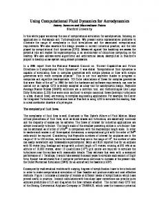
RESULTS AND DISCUSSION As a benchmark problem we used the simulation of a circulating fluidized bed with a square cross-section, corresponding to experiments conducted by Zhou et al. [3,4]. The bed has a square cross-section, 14.6 cm wide, and is 9.14 m in height. The schematic of this setup is shown in Fig. 1a. The solids inlet and outlet are of circular crosssection in the experiments but for geometric simplicity, we have represented them by square cross-section. The area of the square openings and the mass flow rate corresponds to that of the experiments. At a gas velocity of 55 cm/s the drag force on the particles is large enough to blow the particles to the top of the bed and make the bed flow like a fluid or fluidized bed. The particles strike the top wall and some of them exit through the outlet while the rest fall down to encounter the upcoming stream of solids and gases. In the benchmark problem a three-dimensional Cartesian coordinates system was used. The spanwise directions were discretized into 60 cells (0.24 cm, I & K-dimensions) and the
Fig. 1. Schematic of the simulated CFB.
axial, streamwise direction into 400 cells (2.29 cm, J-dimension). The total number of computational cells is around 1.6 million, including the ghost cells; the dynamic memory required is around 1.6 GB. Threedimensional domain decomposition was performed depending on the number of processors for the DMP run. A low-resolution simulation was also carried out with half the resolution in each of the three directions for comparison. In all of the numerical benchmarks reported here for the high-resolution case, two-different preconditioners were used with BICGSTAB linear solver. In one case, red-black coloring in the I-K plane and line-relaxation along J direction was used. With red-black coloring, the number of BICGSTAB iterations is quite insensitive to the number of subdomains used. In the other case, no preconditioner was used. The benchmarks reported here were carried out on one 32-way node of the machine Cheetah at the center for Computational Sciences, Oak Ridge National Laboratory. Cheetah is a 27-node IBM pSeries System, each node with sixteen Power4 chips, a chip consisting of two 1.3 GHz Power4 processors. Each processor has a Level 1 instruction cache of 64 KB and data cache of 32 KB. A Level 2 cache of 1.5 MB on the chip is shared by the two processors, and a Level 3 cache of 32 MB is off-chip. Cheetah’s estimated computational power is 4.5 TeraFLOP/s in the compute partition.
NUMERICAL RESULTS Figure 2 compares the axial-profiles of the time-averaged voidage with the experiments. The voidage is defined as the volume fraction of the gas in any given cell; a voidage of 1 corresponds to pure gas and a voidage of 0 corresponds to pure solid (although this is physically and numerically impossible as the solids go to random close packing with voidage around 0.4, depending on the particle size). The results at three different lateral locations match very well downstream of the inlet region but are not as accurate in the inlet region (although there is some ambiguity in the precise inlet geometry from the limited information in the literature [3,4]). The higher resolution results seem to agree with experiments better than lower resolution ones near the inlet; even higher resolution might be required to resolve the relevant scales in this section. The voidage across the bed (Fig. 3) is predicted well in the upper quarter of the bed. The solids velocity (Fig. 4) is in much better agreement in the near-wall regions of the bed while it is over predicted near the centerline for higher sections in the bed.
Fig. 2. Axial profiles of time-averaged voidage fraction.
Fig. 3. Lateral profiles of time-averaged voidage fraction.
Fig. 4. Axial profiles of time-averaged solids velocity at a height of 5.13 m.
Figure 5 shows instantaneous void fraction snapshots which show recirculation of solids in the vessel. The solids are injected at the base and the high velocity inlet gas carries them to the top (Fig. 5a). The solids accumulate at the bottom. There is also a slight build-up of solids near the top, due to exit effects. Most recirculation of solids is in a narrow band close to the walls (Fig. 5b). The solids accumulated on the top fall down and encounter the upflow at the centerline of bed and tend to move towards the walls (Fig. 5c). Finally in Fig. 5d, the falling solids are mixed with the upcoming solids so as to be recirculated to the top. These figures are shown here as an illustration of the physics that can be captured using numerical simulations; a more detailed analysis of this data will be published in another journal.
Fig. 5. Snapshots of voidage fraction in the Y-Z plane at X = 1.2 cm for different times: (a) 1.12 s, (b) 2.0 s, (c) 2.82 s, and (d) 3.42 s. Here red represents low voidage (0.6) and blue represents high voidage (1.0). Regions of red (low voidage) have higher concentrations of solids and blue corresponds to higher concentrations of air.
PARALLEL RESULTS Table 1 shows the execution times of the code on one node of the IBM SP Cheetah, for ten time steps of the test problem using line relaxation as the preconditioner. An entry in the table gives the running time in seconds on P processors, where P is the product of the number of MPI tasks and the number of threads per task. In all the runs, message passing was through the internal shared memory and not over the network. The runtime on a single processor is not included in the table due to the large problem size which resulted in an extremely long execution time. The runs were carried out several times and the best times are recorded here. The execution times for 8 tasks or 8 threads are not reported here as the run times varied drastically from one run to another run and this behavior could not be explained. Further analysis is required to ascertain the reasons. Table 1 indicates that for a fixed number of processors, the execution time of the code is affected by the mix of the number of MPI tasks and the number of threads per task. For the test problem on 32 processors, 32 one-thread or 16 two-thread MPI tasks give the best combination. In general, the simple rule of “one thread per MPI task, one MPI task per processor” gives the best performance. This general observation is consistent with previous hybrid parallelization efforts on somewhat similar architectures [5,6]. One of the reasons might be the fact that thread creation/destruction is very expensive on the IBM
Table 1. Runtimes (in seconds) for 10 iterations for the case using line relaxation as the preconditioner.
MPI Tasks
1
1 2 4 8 16 32
2
SMP Threads 4
8
16
3188
2012
1125
605
3105
1666
1025
489
350
1709
1121
683
282
1041
554
788
449
233
32 445
235
SPs. Replacing the loop-level SMP model with a program-level SMP model, where the data is decomposed among threads at the beginning of the program, may incur less overhead. Figure 6 compares the SMP and DMP parallel performance. It clearly shows that the DMP performance is far better than that of SMP in the extreme case of hybrid parallelization. Figure 7 captures the essence of the data given in Table 2. It is very evident that DMP parallelization, for this problem on this architecture, is desirable.
35
Speedup (SMP vs. DMP)
30
28
DMP
24
SMP Ideal
Speedup
1 Thread 2 Threads
25 20
4 Threads
16
10
12
5
32 Threads Ideal
0 2
4 0 0
4
8
12
16
20
24
28
32
MPI Tasks/Threads
Fig. 6. SMP/DMP Speedup Comparison.
4
8
16
1 Thread
8
32
Number of Processors (Tasks * Threads)
Ideal
8 Threads 16 Threads
16 Threads
15
20
4 Threads
Speedup
32
Fig. 7. Parallel performance for all the cases (Table 1) with line relaxation as the preconditioner
Table 2 gives the runtimes of the code for the test problem without the use of preconditioner. This required 124 nonlinear iterations for ten time steps compared to the 107 iterations when using the line relaxation preconditioning. However, the code was 20% faster without preconditioning; this may be
Table 2. Runtimes (in seconds) for 10 iterations for the case with no preconditioner.
MPI Tasks
1
1 2 4 8 16 32
2
SMP Threads 4
8
16
2273
1253
768
653
2295
1290
665
480
299
1151
644
369
245
689
473
443
340
191
32 440
186
attributed to the considerably lower cost of an iteration without preconditioning. The speedups are graphically depicted in Figs. 8 and 9. On close observation of speedup data, it can be noted that the shared memory efficiency has dropped further, presumably because the code must take more iterations to converge than with line relaxation. This would increase the number of threads created/destroyed per timestep and explains the poorer performance of the SMP code.
Parallel Performance 35
Speedup (SMP vs. DMP) 30 32
Ideal
20
25 20
1 Thread 2 Threads
15
4 Threads 8 Threads
10
16 Threads 32 Threads Ideal
16
12
0
4
8
12
16
20
24
28
32
MPI Tasks/Threads
Fig. 8. SMP/DMP Speedup Comparison.
2
3
4
Number of Processors (Tasks * Threads)
5
4 Threads
1
0
1 Thread
0
4
16 Threads
5 8
Ideal
Speedup
24
Speedup
DMP SMP
28
Fig. 9. Parallel performance for all the cases (Table 4) with no preconditioner.
The code has to be profiled extensively for a range of problems and also for different architectures before any general conclusions can be made regarding the advantages of DMP code versus a hybrid code. In the present case, MPI communication is memory-to-memory copy as all the processors belong to the same node. Some of the conclusions might change using node-to-node communication.
The above efforts will be continued into next year. In addition, implementation of various non-linear coupled solvers for faster convergence would be explored. The documentation, technical reports related to MFIX, and the latest version of MFIX source code are all available from http://www.mfix.org.
REFERENCES 1. D’Azevedo, E., Pannala, S., Syamlal, M., Gel, A., Prinkey, M., and O’Brien, T., “Parallelization of MFIX: A Multiphase CFD Code for Modeling Fluidized Beds,” Session CP15, Tenth SIAM Conference on Parallel Processing for Scientific Community, Portsmouth, Virginia, March 12–14, 2001. 2. Pannala, S., E. D’Azevedo, T. O’Brien, and M. Syamlal, “Hybrid (mixed SMP/DMP) parallelization of MFIX: A Multiphase CFD code for modeling fluidized beds,” Proceedings of ACM Symposium on Applied Computing, Melbourne, Florida, 9–12 March, 2003. 3. J. Zhou, J. R. Grace, S. Qin, C. M. H. Brereton, C. J. Lim, and J. Zhu, Voidage profiles in a circulating fluidized bed of square cross-section, Chem. Engg. Science, 49 (1994), pp. 3217–3226. 4. J. Zhou, J. R. Grace, S. Qin, C. J. Lim, and C. M. H. Brereton, Particle velocity profiles in a circulating fluidized bed riser of square cross-section, Chem. Engg. Science, 49 (1994), pp. 3217–3226. 5. F. Mathey, P. Blaise, and P. Kloos, OpenMP optimization of a parallel MPI CFD code, Second European Workshop on OpenMP, Murrayfield Conference Centre, Edinburgh, Scotland, U.K., September 14–15, 2000. 6. D. A. Mey and S. Schmidt, From a vector computer to an SMP-Cluster hybrid parallelization of the CFD code PANTA, Second European Workshop on OpenMP, Murrayfield Conference Centre, Edinburgh, Scotland, U.K., September 14–15, 2000.